
![]()
Patterns and Anti-Patterns
In short, no pattern is an isolated entity. Each pattern can exist in the world only to the extent that is supported by other patterns: the larger patterns in which it is embedded, the patterns of the same size that surround it, and the smaller patterns which are embedded in it.
—Christopher Alexander, architect and design theorist
There is an old saying that you shouldn’t try to reinvent the wheel, and honestly, in essence it is a very good saying. But with all such sayings, a modicum of common sense is required for its application. If everyone down through history took the saying literally, your car would have wheels made out of the trunk of a tree (which the MythBusters proved you could do in their “Good Wood” episode), since that clearly could have been one of the first wheel-like machines that was used. If everyone down through history had said “that’s good enough,” driving to Walley World in the family truckster would be a far less comfortable experience.
Over time, however, the basic concept of a wheel has been intact, from rock wheel, to wagon wheel, to steel-belted radials, and even a wheel of cheddar. Each of these is round and able to move by rolling from place A to place B. Each solution follows that common pattern but diverges to solve a particular problem. The goal of a software programmer should be to first try understanding existing techniques and then either use or improve them. Solving the same problem over and over without any knowledge of the past is nuts.
One of the neat things about software design, certainly database design, is that there are base patterns, such as normalization, that we will build upon, but there are additional patterns that are built up starting with normalized tables. That is what this chapter is about, taking the basic structures we have built so far, and taking more and more complex groupings of structures, we will produce more complex, interesting solutions to problems.
Of course, in as much as there are positive patterns that work, there are also negative patterns that have failed over and over down through history. Take personal flight. For many, many years, truly intelligent people tried over and over to strap wings on their arms and fly. They were close in concept, but just doing the same thing over and over was truly folly. Once it was understood how to apply Bernoulli’s principle to building wings and what it would truly take to fly, the Wright brothers applied these principals to produce the first manned flying machine. If you ever happen by Kitty Hawk, NC, you can see the plane and location of that flight. Not an amazing amount has changed between that airplane and today’s airplanes in basic principle. They weren’t required to have their entire body scanned and patted down for that first flight, but the wings worked the same way.
Throughout this book so far, we have covered the basic implementation tools that you can use to assemble solutions that meet your real-world needs. In this chapter, I am going to extend this notion and present a few deeper examples where we assemble a part of a database that deals with common problems that show up in almost any database solution. The chapter is broken up into two major sections, starting with the larger topic, patterns that are desirable to use. The second major section discusses anti-patterns, or patterns that you may frequently see that are not desirable to use (along with the preferred method of solution, naturally).
Desirable Patterns
In this section, I am going to cover a variety of implementation patterns that can be used to solve very common problems that you will frequently encounter. By no means should this be confused with a comprehensive list of the types of problems you may face; think of it instead as a sampling of methods of solving some very common problems.
The patterns and solutions that I will present in the following subsections are as follows:
- Uniqueness: Moving beyond the simple uniqueness we covered in the first chapters of this book, we’ll look at some very realistic patterns of solutions that cannot be implemented with a simple uniqueness constraint.
- Data-driven design: The goal of data-driven design is to never hard-code values that don’t have a fixed meaning. You break down your programming needs into situations that can be based on sets of data values that can be modified without affecting code.
- Historical/temporal: At times it can be very desirable to look at previous versions of data that has changed over time. I will present strategies you can use to view your data at various points in history.
- Hierarchies: A very common need is to implement hierarchies in your data. The most common example is the manager-employee relationship. I will demonstrate the two simplest methods of implementation and introduce other methods that you can explore.
- Images, documents, and other files: There is, quite often, a need to store documents in the database, like a web user’s avatar picture, a security photo to identify an employee, or even documents of many types. We will look at some of the methods available to you in SQL Server and discuss the reasons you might choose one method or another.
- Generalization: We will look at some ways that you need to be careful with how specific you make your tables so that you fit the solution to the needs of the user.
- Storing user-specified data: You can’t always design a database to cover every known future need. I will cover some of the possibilities for letting users extend their database themselves in a manner that can be somewhat controlled by the administrators.
![]() Note I am always looking for other patterns that can solve common issues and enhance your designs (as well as mine). On my web site (www.drsql.org), I may make additional entries available over time, and please leave me comments if you have ideas for more.
Note I am always looking for other patterns that can solve common issues and enhance your designs (as well as mine). On my web site (www.drsql.org), I may make additional entries available over time, and please leave me comments if you have ideas for more.
If you have been reading this book straight through, you likely have gotten the point that uniqueness is a major concern for your design. The fact is, uniqueness is one of the largest problems you will tackle when designing a database, because telling two rows apart from one another can be a very difficult task in some cases.
In this section, we will explore how you can implement different types of uniqueness issues that hit at the heart of the common problems you will come across:
- Selective: Sometimes, we won’t have all of the information for all rows, but the rows where we do have data need to be unique. As an example, consider the driver’s license numbers of employees. No two people can have the same information, but not everyone will necessarily have one, at least not recorded in the database.
- Bulk: Sometimes, we need to inventory items where some of the items are equivalent. For example, cans of corn in the grocery store. You can’t tell each item apart, but you do need to know how many you have.
- Range: Instead of a single value of uniqueness, we often need to make sure that ranges of data don’t overlap, like appointments. For example, take a hair salon. You don’t want Mrs. McGillicutty to have an appointment at the same time as Mrs. Mertz, or no one is going to end up happy. Things are even more important when you are controlling transportation systems.
- Approximate: The most difficult case is the most common, in that it can be really difficult to tell two people apart who come to your company for service. Did two Louis Davidsons purchase toy airplanes yesterday? Possibly. At the same phone number and address, with the same credit card type? Probably not. But another point I have worked to death is that in the database you can’t enforce probably…only definitely.
Uniqueness is one of the biggest struggles in day-to-day operations, particularly in running a company, as it is essential to not offend customers, nor ship them 100 orders of Legos when they actually only placed a single order. We need to make sure that we don’t end up with ten employees with the same SSN (and a visit from the tax man), far fewer cans of corn than we expected, ten appointments at the same time, and so on.
We previously discussed PRIMARY KEY and UNIQUE constraints, but neither of these will fit the scenario where you need to make sure some subset of the data, rather than every row, is unique. For example, say you have an employee table, and each employee can possibly have an insurance policy. The policy numbers must be unique, but the user might not have a policy.
There are three solutions to this problem that are common:
- Filtered indexes: This feature was new in SQL Server 2008. The CREATE INDEX command syntax has a WHERE clause so that the index pertains only to certain rows in the table.
- Indexed view: In versions prior to 2008, the way to implement this is to create a view that has a WHERE clause and then index the view.
- Separate table for NULLable items: A solution that needs noting is to make a separate table for the lower cardinality uniqueness items. So, for example, you might have a table for employees’ insurance policy numbers. In some cases this may be the best solution, but it can lead to proliferation of tables that never really are accessed alone, making it more work than needed. If you designed properly, you will have decided on this in the design phase of the project.
As a demonstration, I will create a schema and table for the human resources employee table with a column for employee number and a column for insurance policy number as well. I will use a database named Chapter8 with default settings for the examples unless otherwise noted.
CREATE SCHEMA HumanResources;
GO
CREATE TABLE HumanResources.Employee
(
    EmployeeId int IDENTITY(1,1) CONSTRAINT PKEmployee primary key,
    EmployeeNumber char(5) NOT NULL
           CONSTRAINT AKEmployee_EmployeeNummer UNIQUE,
    --skipping other columns you would likely have
    InsurancePolicyNumber char(10) NULL
);
Filtered indexes are useful for performance-tuning situations where only a few values are selective, but they also are useful for eliminating values for data protection. Everything about the index is the same as a normal index (indexes will be covered in greater detail in Chapter 10) save for the WHERE clause. So, you add an index like this:
--Filtered Alternate Key (AKF)
CREATE UNIQUE INDEX AKFEmployee_InsurancePolicyNumber ON
                                    HumanResources.Employee(InsurancePolicyNumber)
WHERE InsurancePolicyNumber IS NOT NULL;
Then, create an initial sample row:
INSERT INTO HumanResources.Employee (EmployeeNumber, InsurancePolicyNumber)
VALUES (’A0001’,’1111111111’);
If you attempt to give another employee the same InsurancePolicyNumber
INSERT INTO HumanResources.Employee (EmployeeNumber, InsurancePolicyNumber)
VALUES (’A0002’,’1111111111’);
this fails:
Msg 2601, Level 14, State 1, Line 29
Cannot insert duplicate key row in object ’HumanResources.employee’ with unique index ’AKFEmployee_InsurancePolicyNumber’. The duplicate key value is (1111111111).
Adding the row with the corrected value will succeed:
INSERT INTO HumanResources.Employee (EmployeeNumber, InsurancePolicyNumber)
VALUES (’A0002’,’2222222222’);
However, adding two rows with NULL will work fine:
INSERT INTO HumanResources.Employee (EmployeeNumber, InsurancePolicyNumber)
VALUES (’A0003’,’3333333333’),
       (’A0004’,NULL),
       (’A0005’,NULL);
You can see that this
SELECT *
FROM   HumanResources.Employee;
returns the following:
EmployeeId       EmployeeNumber           InsurancePolicyNumber
---------------- ------------------------ --------------------------------
1                A0001                    1111111111
3                A0002                    2222222222
4                A0003                    3333333333
5                A0004                    NULL
5                A0005                    NULL
The NULL example is the classic example, because it is common to desire this functionality. However, this technique can be used for more than just NULL exclusion. As another example, consider the case where you want to ensure that only a single row is set as primary for a group of rows, such as a primary contact for an account:
CREATE SCHEMA Account;
GO
CREATE TABLE Account.Contact
(
    ContactId   varchar(10) NOT NULL,
    AccountNumber   char(5) NOT NULL, --would be FK in full example
    PrimaryContactFlag bit NOT NULL,
    CONSTRAINT PKContact PRIMARY KEY(ContactId, AccountNumber)
);
Again, create an index, but this time, choose only those rows with PrimaryContactFlag = 1. The other values in the table could have as many other values as you want (of course, in this case, since it is a bit, the values could be only 0 or 1).
CREATE UNIQUE INDEX AKFContact_PrimaryContact
            ON Account.Contact(AccountNumber) WHERE PrimaryContactFlag = 1;
If you try to insert two rows that are primary, as in the following statements that will set both contacts ’fred’ and ’bob’ as the primary contact for the account with account number ’11111’:
INSERT INTO Account.Contact
VALUES (’bob’,’11111’,1);
GO
INSERT INTO Account.Contact
VALUES (’fred’,’11111’,1);
the following error is returned after the second insert:
Msg 2601, Level 14, State 1, Line 73
Cannot insert duplicate key row in object ’Account.Contact’ with unique index ’AKFContact_PrimaryContact’. The duplicate key value is (11111).
To insert the row with ’fred’ as the name and set it as primary (assuming the ’bob’ row was inserted previously), you will need to update the other row to be not primary and then insert the new primary row:
BEGIN TRANSACTION;
UPDATE Account.Contact
SET PrimaryContactFlag = 0
WHERE  accountNumber = ’11111’;
INSERT Account.Contact
VALUES (’fred’,’11111’, 1);
COMMIT TRANSACTION;
Note that in cases like this you would definitely want to use a transaction and error handling in your code so you don’t end up without a primary contact if the INSERT operation fails for some other reason.
Prior to SQL Server 2008, where there were no filtered indexes, the preferred method of implementing this was to create an indexed view with a unique clustered indexes. There are a couple of other ways to do this (such as in a trigger or stored procedure using an EXISTS query, or even using a user-defined function in a CHECK constraint), but the indexed view is the easiest if you cannot use a filtered index (though as of this writing, it is available in all supported versions of SQL Server.
A side effect of the filtered index is that it (like the uniqueness constraints we have used previously) has a very good chance of being useful for searches against the table. The only downside is that the error comes from an index rather than a constraint, so it does not fit into our existing paradigms for error handling.
Bulk Uniqueness
Sometimes, we need to inventory items where some of the items are equivalent in the physical world, for example, cans of corn in the grocery store. Generally, you can’t even tell the cans apart by looking at them (unless they have different expiration dates, perhaps), but knowing how many are in stock is a very common need. Implementing a solution that has a row for every canned good in a corner market would require a very large database even for a very small store. This would be really quite complicated and would require a heck of a lot of rows and data manipulation. It would, in fact, make some queries easier, but it would make data storage a lot more difficult.
Instead of having one row for each individual item, you can implement a row per type of item. This type would be used to store inventory and utilization, which would then be balanced against one another. Figure 8-1 shows a very simplified model of such activity.

Figure 8-1. Simplified inventory model
In the InventoryAdjustment table, you would record shipments coming in, items stolen, changes to inventory after taking inventory (could be more or less, depending on the quality of the data you had), and so forth, and in the ProductSale table (probably a child to sale header or perhaps invoicing table in a complete model), you would record when product is removed or added to inventory from a customer interaction.
The sum of the InventoryAdjustment Quantity value less the sum of ProductSale Quantity value should tell you the amount of product on hand (or perhaps the amount of product you have oversold and need to order posthaste!) In the more realistic case, you would have a lot of complexity for backorders, future orders, returns, and so on, but the base concept is basically the same. Instead of each row representing a single item, each represents a handful of items.
The following miniature design is an example I charge students with when I give my day-long seminar on database design. It is referencing a collection of toys, many of which are exactly alike:
- A certain person was obsessed with his Lego® collection. He had thousands of them and wanted to catalog his Legos both in storage and in creations where they were currently located and/or used. Legos are either in the storage “pile” or used in a set. Sets can either be purchased, which will be identified by an up to five-digit numeric code, or personal, which have no numeric code. Both styles of set should have a name assigned and a place for descriptive notes.
- Legos come in many shapes and sizes, with most measured in 2 or 3 dimensions. First in width and length based on the number of studs on the top, and then sometimes based on a standard height (for example, bricks have height; plates are fixed at 1/3 of 1 brick height unit). Each part comes in many different standard colors as well. Beyond sized pieces, there are many different accessories (some with length/width values), instructions, and so on that can be catalogued.
Example pieces and sets are shown in Figure 8-2.

Figure 8-2. Sample Lego parts for a database
To solve this problem, I will create a table for each set of Legos I own (which I will call Build, since “set” is a bad word for a SQL name, and “build” actually is better anyhow to encompass a personal creation):
CREATE SCHEMA Lego;
GO
CREATE TABLE Lego.Build
(
        BuildId int CONSTRAINT PKBuild PRIMARY KEY,
        Name    varchar(30) NOT NULL CONSTRAINT AKBuild_Name UNIQUE,
        LegoCode varchar(5) NULL, --five character set number
        InstructionsURL varchar(255) NULL --where you can get the PDF of the instructions
);
Then, I’ll add a table for each individual instance of that build, which I will call BuildInstance:
CREATE TABLE Lego.BuildInstance
(
        BuildInstanceId Int CONSTRAINT PKBuildInstance PRIMARY KEY ,
        BuildId Int CONSTRAINT FKBuildInstance$isAVersionOf$LegoBuild
                        REFERENCES Lego.Build (BuildId),
        BuildInstanceName varchar(30) NOT NULL, --brief description of item
        Notes varchar(1000)  NULL, --longform notes. These could describe modifications
                                   --for the instance of the model
        CONSTRAINT AKBuildInstance UNIQUE(BuildId, BuildInstanceName)
);
The next task is to create a table for each individual piece type. I used the term “piece” as a generic version of the different sorts of pieces you can get for Legos, including the different accessories:
CREATE TABLE Lego.Piece
(
        PieceId int CONSTRAINT PKPiece PRIMARY KEY,
        Type    varchar(15) NOT NULL,
        Name    varchar(30) NOT NULL,
        Color   varchar(20) NULL,
        Width int NULL,
        Length int NULL,
        Height int NULL,
        LegoInventoryNumber int NULL,
        OwnedCount int NOT NULL,
        CONSTRAINT AKPiece_Definition UNIQUE (Type,Name,Color,Width,Length,Height),
        CONSTRAINT AKPiece_LegoInventoryNumber UNIQUE (LegoInventoryNumber)
);
Note that I implement the owned count as an attribute of the piece and not as a multivalued attribute to denote inventory change events. In a fully fleshed-out sales model, this might not be sufficient, but for a personal inventory, it would be a reasonable solution. The likely use here will be to update the value as new pieces are added to inventory and possibly to count up loose pieces later and add that value to the ones in sets (which we will have a query for later).
Next, I will implement the table to allocate pieces to different builds:
CREATE TABLE Lego.BuildInstancePiece
(
        BuildInstanceId int NOT NULL,
        PieceId int NOT NULL,
        AssignedCount int NOT NULL,
        CONSTRAINT PKBuildInstancePiece PRIMARY KEY (BuildInstanceId, PieceId)
);
From here, I can load some data. I will load a true Lego item that is available for sale and that I have often given away during presentations. It is a small, black, one-seat car with a little guy in a sweatshirt.
INSERT Lego.Build (BuildId, Name, LegoCode, InstructionsURL)
VALUES  (1,’Small Car’,’3177’,
           ’http://cache.lego.com/bigdownloads/buildinginstructions/4584500.pdf’);
I will create one instance for this, as I personally have only one in my collection (plus some boxed ones to give away):
INSERT Lego.BuildInstance (BuildInstanceId, BuildId, BuildInstanceName, Notes)
VALUES (1,1,’Small Car for Book’,NULL);
Then, I load the table with the different pieces in my collection, in this case, the types of pieces included in the set, plus some extras thrown in. (Note that in a fully fleshed-out design, some of these values would have domains enforced, as well as validations to enforce the types of items that have height, width, and/or lengths. This detail is omitted partially for simplicity, and partially because it might just be too much to implement for a system such as this, based on user needs—though mostly for simplicity of demonstrating the underlying principal of bulk uniqueness in the most compact possible manner.)
INSERT Lego.Piece (PieceId, Type, Name, Color, Width, Length, Height,
                   LegoInventoryNumber, OwnedCount)
VALUES (1, ’Brick’,’Basic Brick’,’White’,1,3,1,’362201’,20),
           (2, ’Slope’,’Slope’,’White’,1,1,1,’4504369’,2),
           (3, ’Tile’,’Groved Tile’,’White’,1,2,NULL,’306901’,10),
           (4, ’Plate’,’Plate’,’White’,2,2,NULL,’302201’,20),
           (5, ’Plate’,’Plate’,’White’,1,4,NULL,’371001’,10),
           (6, ’Plate’,’Plate’,’White’,2,4,NULL,’302001’,1),
           (7, ’Bracket’,’1x2 Bracket with 2x2’,’White’,2,1,2,’4277926’,2),
           (8, ’Mudguard’,’Vehicle Mudguard’,’White’,2,4,NULL,’4289272’,1),
           (9, ’Door’,’Right Door’,’White’,1,3,1,’4537987’,1),
           (10,’Door’,’Left Door’,’White’,1,3,1,’45376377’,1),
           (11,’Panel’,’Panel’,’White’,1,2,1,’486501’,1),
           (12,’Minifig Part’,’Minifig Torso , Sweatshirt’,’White’,NULL,NULL,
                NULL,’4570026’,1),
           (13,’Steering Wheel’,’Steering Wheel’,’Blue’,1,2,NULL,’9566’,1),
           (14,’Minifig Part’,’Minifig Head, Male Brown Eyes’,’Yellow’,NULL, NULL,
                NULL,’4570043’,1),
           (15,’Slope’,’Slope’,’Black’,2,1,2,’4515373’,2),
           (16,’Mudguard’,’Vehicle Mudgard’,’Black’,2,4,NULL,’4195378’,1),
           (17,’Tire’,’Vehicle Tire,Smooth’,’Black’,NULL,NULL,NULL,’4508215’,4),
           (18,’Vehicle Base’,’Vehicle Base’,’Black’,4,7,2,’244126’,1),
           (19,’Wedge’,’Wedge (Vehicle Roof)’,’Black’,1,4,4,’4191191’,1),
           (20,’Plate’,’Plate’,’Lime Green’,1,2,NULL,’302328’,4),
           (21,’Minifig Part’,’Minifig Legs’,’Lime Green’,NULL,NULL,NULL,’74040’,1),
           (22,’Round Plate’,’Round Plate’,’Clear’,1,1,NULL,’3005740’,2),
           (23,’Plate’,’Plate’,’Transparent Red’,1,2,NULL,’4201019’,1),
           (24,’Briefcase’,’Briefcase’,’Reddish Brown’,NULL,NULL,NULL,’4211235’, 1),
           (25,’Wheel’,’Wheel’,’Light Bluish Gray’,NULL,NULL,NULL,’4211765’,4),
           (26,’Tile’,’Grilled Tile’,’Dark Bluish Gray’,1,2,NULL,’4210631’, 1),
           (27,’Minifig Part’,’Brown Minifig Hair’,’Dark Brown’,NULL,NULL,NULL,
               ’4535553’, 1),
           (28,’Windshield’,’Windshield’,’Transparent Black’,3,4,1,’4496442’,1),
           --and a few extra pieces to make the queries more interesting
           (29,’Baseplate’,’Baseplate’,’Green’,16,24,NULL,’3334’,4),
           (30,’Brick’,’Basic Brick’,’White’,4,6,NULL,’2356’,10);
Next, I will assign the 43 pieces that make up the first set (with the most important part of this statement being to show you how cool the row constructor syntax is that was introduced in SQL Server 2008—this would have taken over 20 lines previously):
INSERT INTO Lego.BuildInstancePiece (BuildInstanceId, PieceId, AssignedCount)
VALUES (1,1,2),(1,2,2),(1,3,1),(1,4,2),(1,5,1),(1,6,1),(1,7,2),(1,8,1),(1,9,1),
       (1,10,1),(1,11,1),(1,12,1),(1,13,1),(1,14,1),(1,15,2),(1,16,1),(1,17,4),
       (1,18,1),(1,19,1),(1,20,4),(1,21,1),(1,22,2),(1,23,1),(1,24,1),(1,25,4),
       (1,26,1),(1,27,1),(1,28,1);
Next, I will set up two other minimal builds to make the queries more interesting:
INSERT Lego.Build (BuildId, Name, LegoCode, InstructionsURL)
VALUES  (2,’Brick Triangle’,NULL,NULL);
GO
INSERT Lego.BuildInstance (BuildInstanceId, BuildId, BuildInstanceName, Notes)
VALUES (2,2,’Brick Triangle For Book’,’Simple build with 3 white bricks’);
GO
INSERT INTO Lego.BuildInstancePiece (BuildInstanceId, PieceId, AssignedCount)
VALUES (2,1,3);
GO
INSERT Lego.BuildInstance (BuildInstanceId, BuildId, BuildInstanceName, Notes)
VALUES (3,2,’Brick Triangle For Book2’,’Simple build with 3 white bricks’);
GO
INSERT INTO Lego.BuildInstancePiece (BuildInstanceId, PieceId, AssignedCount)
VALUES (3,1,3);
After the mundane (and quite tedious when done all at once) business of setting up the data is passed, we can count the types of pieces we have in our inventory, and the total number of pieces we have using a query such as this:
SELECT COUNT(*) AS PieceCount, SUM(OwnedCount) AS InventoryCount
FROM  Lego.Piece;
This query returns the following, with the first column giving us the different types:
PieceCount  InventoryCount
----------- --------------
30          111
Here, you start to get a feel for how this is going to be a different sort of solution than the basic relational inventory solution. Instinctively, one expects that a single row represents one thing, but here, you see that, on average, each row represents four different pieces. Following this train of thought, we can group based on the generic type of piece using a query such as
SELECT Type, COUNT(*) AS TypeCount, SUM(OwnedCount) AS InventoryCount
FROM  Lego.Piece
GROUP BY Type;
In these results, you can see that we have 2 types of brick but 30 bricks in inventory, 1 type of baseplate but 4 of them in inventory, and so on:
Type            TypeCount   InventoryCount
--------------- ----------- --------------
Baseplate       1           4
Bracket         1           2
Brick           2           30
Briefcase       1           1
Door            2           2
Minifig Part    4           4
Mudguard        2           2
Panel           1           1
Plate           5           36
Round Plate     1           2
Slope           2           4
Steering Wheel  1           1
Tile            2           11
Tire            1           4
Vehicle Base    1           1
Wedge           1           1
Wheel           1           4
Windshield      1           1
The biggest concern with this method is that users have to know the difference between a row and an instance of the thing the row is modeling. And it gets more interesting where the cardinality of the type is very close to the number of physical items on hand. With 30 types of item and only 111 actual pieces, users querying may not immediately see that they are getting a wrong count. In a system with 20 different products and 1 million pieces of inventory, it will be a lot more obvious.
In the next two queries, I will expand into actual interesting queries that you will likely want to use. First, I will look for pieces that are assigned to a given set, in this case, the small car model that we started with. To do this, we will just join the tables, starting with Build and moving on to BuildInstance, BuildInstancePiece, and Piece. All of these joins are inner joins, since we want items that are included in the set. I use grouping sets (another wonderful feature that comes in handy to give us a very specific set of aggregates—in this case, using the () notation to give us a total count of all pieces).
SELECT CASE WHEN GROUPING(Piece.Type) = 1 THEN ’--Total--’ ELSE Piece.Type END AS PieceType,
                Piece.Color,Piece.Height, Piece.Width, Piece.Length,
           SUM(BuildInstancePiece.AssignedCount) AS ASsignedCount
FROM   Lego.Build
                 JOIN Lego.BuildInstance
                        ON Build.BuildId = BuildInstance.BuildId
                 JOIN Lego.BuildInstancePiece
                        ON BuildInstance.BuildInstanceId =
                                    BuildInstancePiece.BuildInstanceId
                 JOIN Lego.Piece
                        ON BuildInstancePiece.PieceId = Piece.PieceId
WHERE  Build.Name = ’Small Car’
       AND  BuildInstanceName = ’Small Car for Book’
GROUP BY GROUPING SETS((Piece.Type,Piece.Color, Piece.Height, Piece.Width, Piece.Length),
                       ());
This returns the following, where you can see that 43 pieces go into this set:
PieceType       Color                Height      Width       Length      AssignedCount
--------------- -------------------- ----------- ----------- ----------- -------------
Bracket         White                2           2           1           2
Brick           White                1           1           3           2
Briefcase       Reddish Brown        NULL        NULL        NULL        1
Door            White                1           1           3           2
Minifig Part    Dark Brown           NULL        NULL        NULL        1
Minifig Part    Lime Green           NULL        NULL        NULL        1
Minifig Part    White                NULL        NULL        NULL        1
Minifig Part    Yellow               NULL        NULL        NULL        1
Mudguard        Black                NULL        2           4           1
Mudguard        White                NULL        2           4           1
Panel           White                1           1           2           1
Plate           Lime Green           NULL        1           2           4
Plate           Transparent Red      NULL        1           2           1
Plate           White                NULL        1           4           1
Plate           White                NULL        2           2           2
Plate           White                NULL        2           4           1
Round Plate     Clear                NULL        1           1           2
Slope           Black                2           2           1           2
Slope           White                1           1           1           2
Steering Wheel  Blue                 NULL        1           2           1
Tile            Dark Bluish Gray     NULL        1           2           1
Tile            White                NULL        1           2           1
Tire            Black                NULL        NULL        NULL        4
Vehicle Base    Black                2           4           7           1
Wedge           Black                4           1           4           1
Wheel           Light Bluish Gray    NULL        NULL        NULL        4
Windshield      Transparent Black    1           3           4           1
--Total--       NULL                 NULL        NULL        NULL        43
The final query in this section is the more interesting one. A very common question would be, “How many pieces of a given type do I own that are not assigned to a set?” For this, I will use a common table expression (CTE) that gives me a sum of the pieces that have been assigned to a BuildInstance and then use that set to join to the Piece table:
;WITH AssignedPieceCount
AS (
SELECT PieceId, SUM(AssignedCount) AS TotalAssignedCount
FROM   Lego.BuildInstancePiece
GROUP  BY PieceId )
SELECT Type, Name,  Width, Length,Height,
       Piece.OwnedCount - Coalesce(TotalAssignedCount,0) AS AvailableCount
FROM   Lego.Piece
                 LEFT OUTER JOIN AssignedPieceCount
                        on Piece.PieceId =  AssignedPieceCount.PieceId
WHERE Piece.OwnedCount - Coalesce(TotalAssignedCount,0) > 0;
Because the cardinality of the AssignedPieceCount to the Piece table is zero or one to one, we can simply do an outer join and subtract the number of pieces we have assigned to sets from the amount owned. This returns
Type       Name          Width    Length   Height  AvailableCount
---------- ------------- -------- -------- ------- --------------
Brick      Basic Brick   1        3        1       12
Tile       Groved Tile   1        2        NULL    9
Plate      Plate         2        2        NULL    18
Plate      Plate         1        4        NULL    9
Baseplate  Baseplate     16       24       NULL    4
Brick      Basic Brick   4        6        NULL    10
You can expand this basic pattern to almost any bulk uniqueness situation you may have. The calculation of how much inventory you have may be more complex and might include inventory values that are stored daily to avoid massive recalculations (think about how your bank account balance is set at the end of the day, and then daily transactions are added/subtracted as they occur until they too are posted and fixed in a daily balance).
In some cases, uniqueness isn’t uniqueness on the values of a single column set, but rather over the values between values. Very common examples of this include appointment times, college classes, or even teachers/employees who can only be assigned to one location at a time.
For example, consider an appointment time. It has a start and an end, and the start and end ranges of two appointments should not overlap. Suppose we have an appointment with start and end times defined with precision to the second, starting at ’20160712 1:00:00PM’ and ending at ’20160712 1:59:59PM’. To validate that this data does not overlap other appointments, we need to look for rows where any of the following conditions are met, indicating we are double booking appointment times:
- The start or end time for the new appointment falls between the start and end for another appointment.
- The start time for the new appointment is before and the end time is after the end time for another appointment.
We can protect against situations such as overlapping appointment times by employing a trigger and a query that checks for range overlapping. If the aforementioned conditions are not met, the new row is acceptable. We will implement a simplistic example of assigning a doctor to an office. Clearly, other parameters need to be considered, like office space, assistants, and so on, but I don’t want this section to be larger than the allotment of pages for the entire book. First, we create a table for the doctor and another to set appointments for the doctor:
CREATE SCHEMA Office;
GO
CREATE TABLE Office.Doctor
(
        DoctorId        int NOT NULL CONSTRAINT PKDoctor PRIMARY KEY,
        DoctorNumber char(5) NOT NULL CONSTRAINT AKDoctor_DoctorNumber UNIQUE
);
CREATE TABLE Office.Appointment
(
        AppointmentId   int NOT NULL CONSTRAINT PKAppointment PRIMARY KEY,
        --real situation would include room, patient, etc,
        DoctorId        int NOT NULL,
        StartTime       datetime2(0), --precision to the second
        EndTime         datetime2(0),
        CONSTRAINT AKAppointment_DoctorStartTime UNIQUE (DoctorId,StartTime),
        CONSTRAINT AKAppointment_DoctorEndTime UNIQUE (DoctorId,EndTime),
        CONSTRAINT CHKAppointment_StartBeforeEnd CHECK (StartTime <= EndTime),
        CONSTRAINT FKDoctor$IsAssignedTo$OfficeAppointment FOREIGN KEY (DoctorId)
                                            REFERENCES Office.Doctor (DoctorId)
);
Next, we will add some data to our new table. The AppointmentId value 5 will include a bad date range that overlaps another row for demonstration purposes:
INSERT INTO Office.Doctor (DoctorId, DoctorNumber)
VALUES (1,’00001’),(2,’00002’);
INSERT INTO Office.Appointment
VALUES (1,1,’20160712 14:00’,’20160712 14:59:59’),
       (2,1,’20160712 15:00’,’20160712 16:59:59’),
           (3,2,’20160712 8:00’,’20160712 11:59:59’),
           (4,2,’20160712 13:00’,’20160712 17:59:59’),
           (5,2,’20160712 14:00’,’20160712 14:59:59’); --offensive item for demo, conflicts
                                                       --with 4
As far as the declarative constraints can tell, everything is okay, but the following query will check for data conditions between each row in the table to every other row in the table:
SELECT Appointment.AppointmentId,
       Acheck.AppointmentId AS ConflictingAppointmentId
FROM   Office.Appointment
          JOIN Office.Appointment AS ACheck
                ON Appointment.DoctorId = ACheck.DoctorId
        /*1*/     and Appointment.AppointmentId <> ACheck.AppointmentId
        /*2*/     and (Appointment.StartTime BETWEEN ACheck.StartTime and ACheck.EndTime
        /*3*/           or Appointment.EndTime BETWEEN ACheck.StartTime and ACheck.EndTime
        /*4*/           or (Appointment.StartTime < ACheck.StartTime
                            and Appointment.EndTime > ACheck.EndTime));
In this query, I have highlighted four points:
- make sure that we don’t compare the current row to itself, because an appointment will always overlap itself.
- Here, we check to see if the StartTime is between the start and end, inclusive of the actual values.
- Same as 2 for the EndTime.
- Finally, we check to see if any appointment is engulfing an other.
Running the query, we see that
AppointmentId ConflictingAppointmentId
------------- ------------------------
5             4
4             5
The interesting part of these results is that where there is one offending row, there will always be another. If one row is offending in one way, like starting before and ending after another appointment, the conflicting row will have a start and end time between the first appointment’s time. This won’t be a problem, but the shared blame makes the results more interesting to deal with.
Next, we remove the bad row for now:
DELETE FROM Office.Appointment WHERE AppointmentId = 5;
We will now implement a trigger (using the template as defined in Appendix B) that will check for this condition based on the values in new rows being inserted or updated. There’s no need to check deleted rows (even for the update case), because all a delete operation can do is help the situation (even in the case of the update, where you may move an appointment from one doctor to another).
Note that the basis of this trigger is the query we used previously to check for bad values (I usually implement this as two triggers, one for insert and another for update, both having the same code, but it is shown here as one for simplicity of demonstration):
CREATE TRIGGER Office.Appointment$insertAndUpdate
ON Office.Appointment
AFTER UPDATE, INSERT AS
BEGIN
   SET NOCOUNT ON;
   SET ROWCOUNT 0; --in case the client has modified the rowcount
   --use inserted for insert or update trigger, deleted for update or delete trigger
   --count instead of @@rowcount due to merge behavior that sets @@rowcount to a number
   --that is equal to number of merged rows, not rows being checked in trigger
   DECLARE @msg varchar(2000),    --used to hold the error message
   --use inserted for insert or update trigger, deleted for update or delete trigger
   --count instead of @@rowcount due to merge behavior that sets @@rowcount to a number
   --that is equal to number of merged rows, not rows being checked in trigger
           @rowsAffected int = (SELECT COUNT(*) FROM inserted);
   --      @rowsAffected int = (SELECT COUNT(*) FROM deleted);
   --no need to continue on if no rows affected
   IF @rowsAffected = 0 RETURN;
   BEGIN TRY
         --[validation section]
        --if this is an update, but they don’t change times or doctor, don’t check the data
        IF UPDATE(startTime) OR UPDATE(endTime) OR UPDATE(doctorId)
           BEGIN
           IF EXISTS ( SELECT *
                       FROM   Office.Appointment
                                JOIN Office.Appointment AS ACheck
                                    ON Appointment.doctorId = ACheck.doctorId
                                       AND Appointment.AppointmentId <> ACheck.AppointmentId
                                       AND (Appointment.StartTime BETWEEN Acheck.StartTime
                                                                        AND Acheck.EndTime
                                            OR Appointment.EndTime BETWEEN Acheck.StartTime
                                                                        AND Acheck.EndTime
                                            OR (Appointment.StartTime < Acheck.StartTime
                                                 and Appointment.EndTime > Acheck.EndTime))
                              WHERE  EXISTS (SELECT *
                                             FROM   inserted
                                             WHERE  inserted.DoctorId = Acheck.DoctorId))
                   BEGIN
                         IF @rowsAffected = 1
                                 SELECT @msg = ’Appointment for doctor ’ + doctorNumber +
                                                ’ overlapped existing appointment’
                                 FROM   inserted
                                           JOIN Office.Doctor
                                                   ON inserted.DoctorId = Doctor.DoctorId;
                                  ELSE
                                    SELECT @msg = ’One of the rows caused an overlapping ’ +
                                                   ’appointment time for a doctor’;
                        THROW 50000,@msg,16;
                   END;
         END;
          --[modification section]
   END TRY
   BEGIN CATCH
              IF @@TRANCOUNT > 0
                  ROLLBACK TRANSACTION;
              THROW; --will halt the batch or be caught by the caller’s catch block
   END CATCH;
END;
Next, as a refresher, check out the data that is in the table:
SELECT *
FROM   Office.Appointment;
This returns (or at least it should, assuming you haven’t deleted or added extra data)
appointmentId doctorId    startTime              endTime
------------- ----------- ---------------------- ----------------------
1             1           2016-07-12 14:00:00    2016-07-12 14:59:59
2             1           2016-07-12 15:00:00    2016-07-12 16:59:59
3             2           2016-07-12 08:00:00    2016-07-12 11:59:59
4             2           2016-07-12 13:00:00    2016-07-12 17:59:59
This time, when we try to add an appointment for doctorId number 1:
INSERT INTO Office.Appointment
VALUES (5,1,’20160712 14:00’,’20160712 14:59:59’);
this first attempt is blocked because the row is an exact duplicate of the start time value. The most common error that will likely occur in a system such as this is trying to duplicate something, usually by accident.
Msg 2627, Level 14, State 1, Line 2
Violation of UNIQUE KEY constraint ’AKOfficeAppointment_DoctorStartTime’. Cannot insert duplicate key in object ’Office.Appointment’. The duplicate key value is (1, 2016-07-12 14:00:00).
Next, we check the case where the appointment fits wholly inside of another appointment:
INSERT INTO Office.Appointment
VALUES (5,1,’20160712 14:30’,’20160712 14:40:59’);
This fails and tells us the doctor for whom the failure occurred:
Msg 50000, Level 16, State 16, Procedure appointment$insertAndUpdate, Line 48
Appointment for doctor 00001 overlapped existing appointment
Then, we test for the case where the entire appointment engulfs another appointment:
INSERT INTO Office.Appointment
VALUES (5,1,’20160712 11:30’,’20160712 17:59:59’);
This quite obediently fails, just like the other case:
Msg 50000, Level 16, State 16, Procedure appointment$insertAndUpdate, Line 48
Appointment for doctor 00001 overlapped existing appointment
And, just to drive home the point of always testing your code extensively, you should always test the greater-than-one-row case, and in this case, I included rows for both doctors:
INSERT into Office.Appointment
VALUES (5,1,’20160712 11:30’,’20160712 15:59:59’),
       (6,2,’20160713 10:00’,’20160713 10:59:59’);
This time, it fails with our multirow error message:
Msg 50000, Level 16, State 16, Procedure appointment$insertAndUpdate, Line 48
One of the rows caused an overlapping appointment time for a doctor
Finally, add two rows that are safe to add:
INSERT INTO Office.Appointment
VALUES (5,1,’20160712 10:00’,’20160712 11:59:59’),
       (6,2,’20160713 10:00’,’20160713 10:59:59’);
This will (finally) work. Now, test failing an update operation:
UPDATE Office.Appointment
SET    StartTime = ’20160712 15:30’,
       EndTime = ’20160712 15:59:59’
WHERE  AppointmentId = 1;
This fails like it should:
Msg 50000, Level 16, State 16, Procedure appointment$insertAndUpdate, Line 38
Appointment for doctor 00001 overlapped existing appointment
If this seems like a lot of work, it is. And in reality, whether or not you actually implement this solution in a trigger is going to be determined by exactly what it is you are doing. However, the techniques of checking range uniqueness can clearly be useful if only to check existing data is correct, because in some cases, what you may want to do is to let data exist in intermediate states that aren’t pristine and then write checks to “certify” that the data is correct before closing out a day.
Instead of blocking the operation, the trigger could update rows to tell the user that it overlaps. Or you might even get more interesting and let the algorithms involve prioritizing certain conditions above other appointments. Maybe a checkup gets bumped for a surgery, marked to reschedule. Realistically, it may be that the user can overlap appointments all they want, and then at the close of business, a query such as the one that formed the basis of the trigger is executed by the administrative assistant, who then clears up any scheduling issues manually. In this section, I’ve shown you a pattern to apply to prevent range overlaps if that is the desired result. It is up to the requirements to lead you to exactly how to implement.
The most difficult case of uniqueness is actually quite common, and it is usually the most critical to get right. It is also a topic far too big to cover with a coded example, because in reality, it is more of a political question than a technical one. For example, if two people call in to your company from the same phone number and say their name is Abraham Lincoln, are they the same person or are they two aliases someone is using? (Or one alias and one real name?) Whether you can call them the same person is a very important decision and one that is based largely on the industry you are in, made especially tricky due to privacy laws (if you give one person who claims to be Abraham Lincoln the data of the real Abraham Lincoln, well, that just isn’t going to be good no matter what your privacy policy is or which laws that govern privacy apply). I don’t talk much about privacy laws in this book, mostly because that subject is very messy, but also because dealing with privacy concerns is
- Largely just an extension of the principles I have covered so far, and will cover in the next chapter on security
- Widely varied by industry and type of data you need to store
- Changing faster than a printed book can cover
- Different depending on what part of the world you are reading this book in
The principles of privacy are part of what makes the process of identification so difficult. At one time, companies would just ask for a customer’s Social Security number and use that as identification in a very trusting manner. Of course, no sooner does some value become used widely by lots of organizations than it begins to be abused. (Chapter 9 will expand a little bit on this topic as we talk about encryption technologies, but encryption is another wide topic for which the best advice is to make sure you are doing as much or more as is required.)
So the goal of your design is to work at getting your customer to use an identifier to help you distinguish them from another customer. This customer identifier will be used, for example, as a login to the corporate web site, for the convenience card that is being used by so many businesses, and also likely on any correspondence. The problem is how to gather this information. When a person calls a bank or doctor, the staff member answering the call always asks some random questions to better identify the caller. For many companies, it is impossible to force the person to give information, so it is not always possible to force customers to uniquely identify themselves. You can entice them to identify themselves, such as by issuing a customer savings card, or you can just guess from bits of information that can be gathered from a web browser, telephone number, and so on. Even worse, what if someone signs up twice for a customer number? Can you be sure that it is the same person, then?
So the goal becomes to match people to the often-limited information they are willing to provide. Generally speaking, you can try to gather as much information as possible from people, such as
- Name
- Address, even partial
- Phone number(s)
- Payment method
- E-mail address(es)
And so on. Then, depending on the industry, you determine levels of matching that work for you. Lots of methods and tools are available to you, from standardization of data to make direct matching possible, fuzzy matching, and even third-party tools that will help you with the matches. The key, of course, is that if you are going to send a message alerting of a sale to repeat customers, only a slight bit of a match might be necessary, but if you are sending personal information, like how much money they have spent, a very deterministic match ought to be done. Identification of multiple customers in your database that are actually the same customer is the holy grail of marketing, but it is achievable given you respect your customer’s privacy and use their data in a safe manner.
Data-Driven Design
One of the worst practices I see some programmers get in the habit of doing is programming using specific values, to force a specific action. For example, they will get requirements that specify that for customers 1 and 2, we need to do action A, and for customer 3, we need to do action B. So they go in and code the following:
IF @customerId in (’1’, ’2’)
    Do ActionA(@customerId);
ELSE IF @customerId in (’3’)
    Do ActionB(@customerId);
It works, so they breathe a sigh of relief and move on. But the next day, they get a request that customer 4 should be treated in the same manner as customer 3. They don’t have time to do this request immediately because it requires a code change, which requires testing. So a month later, they add ’4’ to the code, test it, deploy it, and claim it required 40 hours of IT time.
This is clearly not optimal, so the next best thing is to determine why we are doing ActionA or ActionB. We might determine that for CustomerType: ’Great’, we do ActionA, but for ’Good’, we do ActionB. So you could code
IF @customerType = ’Great’
    Do ActionA(@customerId);
ELSE IF @customerType = ’Good’
    Do ActionB(@customerId);
Now adding another customer to these groups is a fairly simple case. You set the customerType column to Great or Good, and one of these actions occurs in you code automatically. But (as you might hear on any infomercial) you can do better! The shortcoming in this design is now how do you change the treatment of good customers if you want to have them do ActionA temporarily? In some cases, the answer is to add to the definition of the customerType table and add a column to indicate what action to take. So you might code:
--In real table, expand ActionType to be a more descriptive value or a domain of its own
CREATE SCHEMA Customers;
GO
CREATE TABLE Customers.CustomerType
(
        CustomerType    varchar(20) NOT NULL CONSTRAINT PKCustomerType PRIMARY KEY,
        Description     varchar(1000) NOT NULL,
        ActionType      char(1) NOT NULL CONSTRAINT CHKCustomerType_ActionType_Domain
                                               CHECK (ActionType in (’A’,’B’))
);
Now, the treatment of this CustomerType can be set at any time to whatever the user decides. The only time you may need to change code (requiring testing, downtime, etc.) is if you need to change what an action means or add a new one. Adding different types of customers, or even changing existing ones, would be a nonbreaking change, so no testing is required.
The basic goal should be that the structure of data should represent the requirements, so rules are enforced by varying data, not by having to hard-code special cases. Flexibility at the code level is ultra important, particularly to your support staff. In the end, the goal of a design should be that changing configuration should not require code changes, so create attributes that will allow you to configure your data and usage.
![]() Note In the code project part of the downloads for this chapter, you will find a coded example of data-driven design that demonstrates these principals in a complete, SQL coded solution.
Note In the code project part of the downloads for this chapter, you will find a coded example of data-driven design that demonstrates these principals in a complete, SQL coded solution.
One pattern that is quite often needed is to be able to see how a row looked at a previous point in time. For example, when did Employee 100001’s salary change? When did Employee 2010032’s insurance start? In some cases, you need to capture changes using a column in a table. For example, take the Employee table we used in the “Selective Uniqueness” section (if you are following along, this table already exists in the database, so you don’t need to re-create it):
CREATE TABLE HumanResources.Employee
(
    EmployeeId int IDENTITY(1,1) CONSTRAINT PKEmployee primary key,
    EmployeeNumber char(5) NOT NULL
           CONSTRAINT AKEmployee_EmployeeNummer UNIQUE,
    InsurancePolicyNumber char(10) NULL
);
CREATE UNIQUE INDEX AKFEmployee_InsurancePolicyNumber ON
                                    HumanResources.Employee(InsurancePolicyNumber)
                                    WHERE InsurancePolicyNumber IS NOT NULL;
One method of answering the question of when the insurance number changed would be to add
ALTER TABLE HumanResources.Employee
     ADD InsurancePolicyNumberChangeTime datetime2(0);
Possibly with the addition of who changed the row. It could be managed with a trigger, or from the interface code. If you are dealing with a single column that needs to be verified, this is a great way to handle this need. But if you really want to see how all of the columns of a table have changed over time (or a larger subset than one for sure), there are two techniques using T-SQL that are quite popular:
- Using a trigger: Using a fairly simple trigger, we can capture changes to the row and save them in a separate table. The benefit of this method over the next method is that it does not need to capture change for all columns.
- Using temporal extensions: These are available in SQL Server 2016 and allow you to let the engine capture the changes to a table. The major benefit is that there is syntax that allows you to query the changed data in a quite simple manner.
In this section I will demonstrate both methods using the table we have created. Before starting each example, I will use the following code to reset the tables of data:
TRUNCATE TABLE HumanResources.Employee;
INSERT INTO HumanResources.Employee (EmployeeNumber, InsurancePolicyNumber)
VALUES (’A0001’,’1111111111’),
        (’A0002’,’2222222222’),
        (’A0003’,’3333333333’),
        (’A0004’,NULL),
        (’A0005’,NULL),
        (’A0006’,NULL);
Note that neither version of this pattern is generally a version of auditing. The trigger model can be used more for auditing by adding columns in for who made the change, but there are better auditing tools built in to find people doing incorrect things with your data. This pattern is specifically set up to show changes in data, and it is not beyond reasonability that you might change history to cover up mistakes that were data related. Audits should never be changed or they will quickly be considered unreliable.
Using a Trigger to Capture History
While temporal support is a big new feature of SQL Server 2016, it does not take away the value of using a trigger to capture history. In this section, our goal is simply to see a log of modified rows, or rows that have been deleted from the table. For this exercise, we will start by creating a schema for the history that corresponds to the name of the schema that owns the data. This will allow you to manage security at the schema level for history different than for the base table. So giving the user SELECT rights of a schema to read the data does not give them rights to see the history data.
CREATE SCHEMA HumanResourcesHistory;
Next we will create a parallel history table in the new schema that has all of the columns of the original table, along with a few management columns, which have explanations in the following code:
CREATE TABLE HumanResourcesHistory.Employee
(
    --Original columns
    EmployeeId int NOT NULL,
    EmployeeNumber char(5) NOT NULL,
    InsurancePolicyNumber char(10) NULL,
    --WHEN the row was modified
    RowModificationTime datetime2(7) NOT NULL,
    --WHAT type of modification
    RowModificationType varchar(10) NOT NULL CONSTRAINT
               CHKEmployeeSalary_RowModificationType
                      CHECK (RowModificationType IN (’UPDATE’,’DELETE’)),
    --tiebreaker for seeing order of changes, if rows were modified rapidly
    RowSequencerValue bigint IDENTITY(1,1) --use to break ties in RowModificationTime
);
Next, we create the following trigger. The basic flow is to determine the type of operation, then write the contents of the deleted table to the history table we have previously created.
CREATE TRIGGER HumanResources.Employee$HistoryManagementTrigger
ON HumanResources.Employee
AFTER UPDATE, DELETE AS
BEGIN
   SET NOCOUNT ON;
   SET ROWCOUNT 0; --in case the client has modified the rowcount
   --use inserted for insert or update trigger, deleted for update or delete trigger
   --count instead of @@rowcount due to merge behavior that sets @@rowcount to a number
   --that is equal to number of merged rows, not rows being checked in trigger
   DECLARE @msg varchar(2000),    --used to hold the error message
           @rowsAffected int = (SELECT COUNT(*) FROM deleted);
   IF @rowsAffected = 0 RETURN;
   DECLARE @RowModificationType char(6);
   SET @RowModificationType = CASE WHEN EXISTS (SELECT * FROM inserted) THEN ’UPDATE’
                                                          ELSE ’DELETE’ END;
   BEGIN TRY
       --[validation section]
       --[modification section]
       --write deleted rows to the history table
       INSERT  HumanResourcesHistory.Employee(EmployeeId,EmployeeNumber,InsurancePolicyNumber,
                                              RowModificationTime,RowModificationType)
       SELECT EmployeeId,EmployeeNumber,InsurancePolicyNumber,
              SYSDATETIME(), @RowModificationType
       FROM   deleted;
   END TRY
   BEGIN CATCH
       IF @@TRANCOUNT > 0
             ROLLBACK TRANSACTION;
       THROW; --will halt the batch or be caught by the caller’s catch block
     END CATCH;
END;
Now let’s make a few changes to the data in the table. As a reminder, here is the data we start with:
SELECT *
FROM   HumanResources.Employee;
This shows us our base data:
----------- -------------- ---------------------
1           A0001          1111111111
2           A0002          2222222222
3           A0003          3333333333
4           A0004          NULL
5           A0005          NULL
6           A0006          NULL
Next, update EmployeeId = 4 and set that it has insurance:
UPDATE HumanResources.Employee
SET    InsurancePolicyNumber = ’4444444444’
WHERE  EmployeeId = 4;
You can see the change and the history here:
SELECT *
FROM   HumanResources.Employee
WHERE  EmployeeId = 4;
SELECT *
FROM   HumanResourcesHistory.Employee
WHERE  EmployeeId = 4;
EmployeeId  EmployeeNumber InsurancePolicyNumber
----------- -------------- ---------------------
4           A0004          4444444444
EmployeeId  EmployeeNumber InsurancePolicyNumber RowModificationTime
----------- -------------- --------------------- ---------------------------
4           A0004          NULL                  2016-05-07 20:26:38.4578351
RowModificationType RowSequencerValue
------------------- --------------------
UPDATE              1
Now let’s update all of the rows where there is an insurance policy to a new format, and delete EmployeeId = 6. I updated all rows so we can see in the history what happens when a row is updated and does not actually change:
UPDATE HumanResources.Employee
SET  InsurancePolicyNumber = ’IN’ + RIGHT(InsurancePolicyNumber,8);
DELETE HumanResources.Employee
WHERE EmployeeId = 6;
Then check out the data:
SELECT *
FROM   HumanResources.Employee
ORDER BY EmployeeId;
--limiting output for formatting purposes
SELECT EmployeeId, InsurancePolicyNumber, RowModificationTime, RowModificationType
FROM   HumanResourcesHistory.Employee
ORDER BY EmployeeId,RowModificationTime,RowSequencerValue;
This returns
EmployeeId  EmployeeNumber InsurancePolicyNumber
----------- -------------- ---------------------
1           A0001          IN11111111
2           A0002          IN22222222
3           A0003          IN33333333
4           A0004          IN44444444
5           A0005          NULL
EmployeeId   InsurancePolicyNumber RowModificationTime         RowModificationType
-----------  --------------------- --------------------------- -------------------
1            1111111111            2016-05-07 20:27:59.8852810 UPDATE
2            2222222222            2016-05-07 20:27:59.8852810 UPDATE
3            3333333333            2016-05-07 20:27:59.8852810 UPDATE
4            NULL                  2016-05-07 20:26:38.4578351 UPDATE
4            4444444444            2016-05-07 20:27:59.8852810 UPDATE
5            NULL                  2016-05-07 20:27:59.8852810 UPDATE
6            NULL                  2016-05-07 20:27:59.8852810 UPDATE
6            NULL                  2016-05-07 20:27:59.9347658 DELETE
Using this data, you can see the progression of what has happened to the data, starting from the time the trigger was added, including seeing rows that have been deleted. It is a well-worn method to capture history, but it is very hard to work with in your queries to look back on history.
Using Temporal Extensions to Manage History
Temporal extensions will provide the same basic information that we provided using the trigger in the previous section, but there is one major difference: query support. If you want to see the current data, there is no change to your query. But if you want to see how the data looked at a particular point in time, the only change to your query is to specify the time (or time range) for which you want to see history.
The biggest limitation on temporal tables is that the history copy must version all columns in the table. So if you are using an nvarchar(max) or even text (which you really shouldn’t be!), it will work, but you could incur massive performance issues if your values are very large. Even in-memory tables support temporal, but version table will be an on-disk table.
There are other limitations, such as requiring a primary key; TRUNCATE TABLE not allowed; foreign key CASCADE operations are not allowed on the table; INSTEAD OF triggers are not allowed on the table; and replication use is limited. Several other configuration limitations are included in this more complete list of considerations and limitations from Microsoft: msdn.microsoft.com/en-us/library/mt604468.aspx. However, the limitations are not terribly constraining if you need the DML extensions described later in the section.
I will continue to use the HumanResources table we used in the previous section, but I will reset the data and drop the history table from the previous section:
TRUNCATE TABLE HumanResources.Employee;
INSERT INTO HumanResources.Employee (EmployeeNumber, InsurancePolicyNumber)
VALUES (’A0001’,’1111111111’),
       (’A0002’,’2222222222’),
       (’A0003’,’3333333333’),
       (’A0004’,NULL),
       (’A0005’,NULL),
       (’A0006’,NULL);
GO
DROP TABLE HumanResourcesHistory.Employee;
DROP TRIGGER HumanResources.Employee$HistoryManagementTrigger;
In the following subsections, I will cover configuring temporal extensions, along with how you can coordinate changes to multiple rows and how you can change history if needed.
Configuring Temporal Extensions
Now let’s add temporal extensions to the HumanResources.Employee table. To do this, you are required to have two columns in the table, one for a start time, which you will see often in the documentation as SysStartTime, and one for an end time, usually named SysEndTime. I will use a naming standard that matches my normal standard so they match the table. These time range columns must be datetime2, but they can be any precision from 0 to 7. These values are used to denote the start and end time that the row is valid, so when we query the rows using temporal extensions, the one active row can be picked. The precision of the column will determine how many versions you can have per second. If datetime2(0) is used, then you can have one version per second; if datetime2(7), then ~9999999 versions per second. While it is not likely that many readers will have such needs to track changes to this deep level, I tend to use (7) just because it feels like it is safer, if more difficult to type. (For this book I will use datetime2(1) to allow for the limited amount of text real estate I have available.)
The following code snippet adds the columns and the settings that we will use once we turn on system versioning (then drops the temporary constraints):
ALTER TABLE HumanResources.Employee
ADD
    RowStartTime datetime2(1) GENERATED ALWAYS AS ROW START NOT NULL
           --HIDDEN can be specified
           --so temporal columns don’t show up in SELECT * queries
           --This default will start the history of all existing rows at the
           --current time (system uses UTC time for these values)
        CONSTRAINT DFLTDelete1 DEFAULT (SYSUTCDATETIME()),
    RowEndTime datetime2(1) GENERATED ALWAYS AS ROW END NOT NULL --HIDDEN
          --data needs to be the max for the datatype
        CONSTRAINT DFLTDelete2 DEFAULT (CAST(’9999-12-31 23:59:59.9’ AS datetime2(1)))
  , PERIOD FOR SYSTEM_TIME (RowStartTime, RowEndTime);
GO
--DROP the constraints that are just there due to data being in the table
ALTER TABLE HumanResources.Employee
        DROP CONSTRAINT DFLTDelete1;
ALTER TABLE HumanResources.Employee
         DROP CONSTRAINT DFLTDelete2;
The GENERATED ALWAYS AS ROW START and END pair tells the system to set the value when the table is completely configured for temporal support. If you are creating a new table and want to turn on temporal extensions, you will use the same columns and settings in the CREATE TABLE statement, but you won’t need the DEFAULT constraints.
The next step is to create a version table. There are two ways to do this. The easiest is to just let SQL Server build it for you. You can either specify a name or let SQL Server pick one for you. For example, if we want SQL Server to create the history table, we will just use
ALTER TABLE HumanResources.Employee
         SET (SYSTEM_VERSIONING = ON);
Now you can look in the system metadata and see what has been added:
SELECT  tables.object_id AS baseTableObject,
        CONCAT(historySchema.name,’.’,historyTable.name) AS historyTable
FROM    sys.tables
          JOIN sys.schemas
              ON schemas.schema_id = tables.schema_id
          LEFT OUTER JOIN sys.tables AS historyTable
                 JOIN sys.schemas AS historySchema
                       ON historySchema.schema_id = historyTable.schema_id
            ON TABLES.history_table_id = historyTable.object_id
WHERE   schemas.name = ’HumanResources’
  AND   tables.name = ’Employee’;
This returns something like the following, with almost certainly a different base table object_id:
baseTableObject historyTable
--------------- ----------------------------------------------------------
1330103779      HumanResources.MSSQL_TemporalHistoryFor_1330103779
This leads to a predictable but ugly name. The table will have the same columns as the base table, but will have a few differences that we will look at later when we cover creating your own table and modifying the data in the table to use previous historical data you have saved off.
While there may not be a reason all that often to look at the temporal tables, it will be useful to be able to correlate the names of the tables without knowing the object_id. So let’s go ahead and name the table ourselves in the DDL. First we need to disconnect the history table that was created and drop it. Before you can do much to the base table, in fact, you will have to turn off the system versioning:
ALTER TABLE HumanResources.Employee
         SET (SYSTEM_VERSIONING = OFF);
DROP TABLE HumanResources.MSSQL_TemporalHistoryFor_1330103779;
Now let’s specify the table name. If it is an existing table, there will be more to do, in that you may want to backfill up history (like if you were previously trigger to capture history). Just like in the trigger method, I will use a different schema for the history tables, but you can put it in the same schema if so desired (you always have to specify the schema in the HISTORY_TABLE clause):
ALTER TABLE HumanResources.Employee
                                     --must be in the same database
         SET (SYSTEM_VERSIONING = ON (HISTORY_TABLE = HumanResourcesHistory.Employee));
Taking a look at the metadata query we ran earlier, you can see that the history table has been set to a much better table name:
baseTableObject historyTable
--------------- --------------------------------------
1330103779      HumanResourcesHistory.Employee
I will cover security in more detail in Chapter 9, but understand that the user will need rights to the history table in order to SELECT the temporal aspects of the table. A user can modify the contents of the table with just INSERT, UPDATE, and/or DELETE rights.
Now you have configured the HumanResources.Employee table to capture history, starting with the time period of your ALTER statement to add the columns to the table. Check the table’s content using a SELECT statement:
SELECT *
FROM   HumanResources.Employee;
This returns
EmployeeId  EmployeeNumber InsurancePolicyNumber RowStartTime          RowEndTime
----------- -------------- --------------------- --------------------- ---------------------
1           A0001          1111111111            2016-05-10 02:35:49.1 9999-12-31 23:59:59.9
2           A0002          2222222222            2016-05-10 02:35:49.1 9999-12-31 23:59:59.9
3           A0003          3333333333            2016-05-10 02:35:49.1 9999-12-31 23:59:59.9
4           A0004          NULL                  2016-05-10 02:35:49.1 9999-12-31 23:59:59.9
5           A0005          NULL                  2016-05-10 02:35:49.1 9999-12-31 23:59:59.9
6           A0006          NULL                  2016-05-10 02:35:49.1 9999-12-31 23:59:59.9
You can see the new columns added for RowStart… and RowEnd… Time. Using these timeframes, you will be able to see the data at given points of time. So if you wanted to see how the table would have looked on the fourth of May, use the FOR SYSTEM_TIME clause on the table in the FROM clause using AS OF a current point in time, in our case where RowStartTime >= PassedValue > RowEndTime. There are four others: FROM, BETWEEN, CONTAINED IN, and ALL. I will mostly make use of AS OF and ALL in the book, as usually I want to see data at a point in time, or I want to see all history to show you what has changed.
SELECT *
FROM   HumanResources.Employee FOR SYSTEM_TIME AS OF ’2016-05-04’;
This returns nothing, as the RowStart and End do not include that time period for any row in the table. The following query will (based on the data as I have it in my sample table) return the same as the previous query to get all rows in the base table, since 2016-05-11 is after all of the RowStartTime values in the base table:
SELECT *
FROM   HumanResources.Employee FOR SYSTEM_TIME AS OF ’2016-05-11’;
Dealing with Temporal Data One Row at a Time
When your application modifies a single row in a table that has temporal extensions enabled, there really isn’t much you need to consider in your application. Every INSERT, UPDATE, and DELETE operation will just capture changes, and let you query each table that is involved in the operation at a point in time. You can use the FROM FOR SYSTEM_TIME clause on any statement where a FROM clause makes sense. And you can use it on all tables that are used in a query, or just some. For example, the following is perfectly acceptable:
FROM  Table1
        JOIN Table2 FOR SYSTEM_TIME AS OF ’Time Literal’
                    ON ...
        JOIN Table3 FOR SYSTEM_TIME AS OF ’Time Literal’
                    ON ...
And you can even do this:
FROM  Table1 FOR SYSTEM_TIME AS OF ’Time Literal 1’
        JOIN Table1 as DifferentLookAtTable1 FOR SYSTEM_TIME AS OF ’Time Literal 2’
                    ON ...
In the next section we will look more at coordinating modifications on multiple rows (in the same or multiple tables), but in this section, let’s look at the basic mechanics.
First let’s modify some data, to show what this looks like:
UPDATE HumanResources.Employee
SET    InsurancePolicyNumber = ’4444444444’
WHERE  EmployeeId = 4;
So let’s look at the data:
SELECT *
FROM   HumanResources.Employee
WHERE  EmployeeId = 4;
As expected:
EmployeeId  EmployeeNumber InsurancePolicyNumber RowStartTime          RowEndTime
----------- -------------- --------------------- --------------------- ---------------------
4           A0004          4444444444            2016-05-10 02:46:58.3 9999-12-31 23:59:59.9
But check just before the RowStartTime (.3 seconds to be precise):
SELECT *
FROM   HumanResources.Employee FOR SYSTEM_TIME AS OF ’2016-05-10 02:46:58’
WHERE  EmployeeId = 4;
and the data looks just the same as it did pre-UPDATE execution:
EmployeeId  EmployeeNumber InsurancePolicyNumber RowStartTime          RowEndTime
----------- -------------- --------------------- --------------------- ---------------------
4           A0004          NULL                  2016-05-10 02:35:49.1 2016-05-10 02:46:58.3
This is where ALL comes in handy, so you can see all of the changes:
SELECT *
FROM   HumanResources.Employee FOR SYSTEM_TIME ALL
ORDER  BY EmployeeId, RowStartTime;
This returns all of the valid history rows (ones where RowStartTime <> RowEndTime, a situation that I will cover in a moment), including previous versions of data:
EmployeeId  EmployeeNumber InsurancePolicyNumber RowStartTime          RowEndTime
----------- -------------- --------------------- --------------------- ---------------------
1           A0001          1111111111            2016-05-10 02:35:49.1 9999-12-31 23:59:59.9
2           A0002          2222222222            2016-05-10 02:35:49.1 9999-12-31 23:59:59.9
3           A0003          3333333333            2016-05-10 02:35:49.1 9999-12-31 23:59:59.9
4           A0004          NULL                  2016-05-10 02:35:49.1 2016-05-10 02:46:58.3
4           A0004          4444444444            2016-05-10 02:46:58.3 9999-12-31 23:59:59.9
5           A0005          NULL                  2016-05-10 02:35:49.1 9999-12-31 23:59:59.9
6           A0006          NULL                  2016-05-10 02:35:49.1 9999-12-31 23:59:59.9
Now, let’s delete EmployeeId = 6 (we don’t like him…he ate our gluten-free, 10-calorie cupcake):
DELETE HumanResources.Employee
WHERE  EmployeeId = 6;
Then check out the data:
SELECT *
FROM   HumanResources.Employee FOR SYSTEM_TIME ALL
WHERE  EmployeeId = 6
ORDER  BY EmployeeId, RowStartTime;
Now you can see that the RowEndTime value is not ’9999-12-31 23:59:59.9’ but is set to the time of the DELETE:
EmployeeId  EmployeeNumber InsurancePolicyNumber RowStartTime          RowEndTime
----------- -------------- --------------------- --------------------- ---------------------
6           A0006          NULL                  2016-05-10 02:35:49.1 2016-05-10 05:36:28.3
The reasons is that at that point in time, it did exist, but now it doesn’t. If he (EmployeeId = 6) apologizes and gets added back with the same surrogate key value, there would be a gap in time sequence that would correspond to the time when the row was removed.
A word of caution about versions. When the table has SYSTEM_VERSIONING ON, every update will cause a new version, even if no data changes. So,
UPDATE HumanResources.Employee
SET    EmployeeNumber = EmployeeNumber
WHERE  EmployeeId = 4;
is going to lead to a new version:
SELECT *
FROM   HumanResources.Employee FOR SYSTEM_TIME ALL
WHERE  EmployeeId = 4
ORDER  BY EmployeeId, RowStartTime;
This returns
EmployeeId  EmployeeNumber InsurancePolicyNumber RowStartTime          RowEndTime
----------- -------------- --------------------- --------------------- ---------------------
4           A0004          NULL                  2016-05-10 02:35:49.1 2016-05-10 02:46:58.3
4           A0004          4444444444            2016-05-10 02:46:58.3 2016-05-10 02:54:11.8
4           A0004          4444444444            2016-05-10 02:54:11.8 2016-05-10 02:59:36.6
But you can see that there is no difference between the second row in the output and the third. Now, let’s do five updates, immediately following one another using SSMS’s GO # extension:
UPDATE HumanResources.Employee
SET    EmployeeNumber = EmployeeNumber
WHERE  EmployeeId = 4;
GO 5
Looking at the data
SELECT *
FROM   HumanResources.Employee FOR SYSTEM_TIME ALL
WHERE  EmployeeId = 4
ORDER  BY EmployeeId, RowStartTime;
we see only five rows, but there should be eight, right? In this case, some rows were updated within what the system registered as the same time, so they are hidden. You can only see them in the history table:
EmployeeId  EmployeeNumber InsurancePolicyNumber RowStartTime          RowEndTime
----------- -------------- --------------------- --------------------- ---------------------
4           A0004          NULL                  2016-05-10 02:35:49.1 2016-05-10 02:46:58.3
4           A0004          4444444444            2016-05-10 02:46:58.3 2016-05-10 02:54:11.8
4           A0004          4444444444            2016-05-10 02:54:11.8 2016-05-10 02:59:36.6
4           A0004          4444444444            2016-05-10 02:59:36.6 2016-05-10 03:01:06.5
4           A0004          4444444444            2016-05-10 03:01:06.5 9999-12-31 23:59:59.9
Three of the rows have the same RowStart and RowEnd times (your mileage may vary, depending on the precision of your row times; sometimes I did not see this phenomenon, but most every time I did, even using datetime2(7)):
SELECT *
FROM   HumanResourcesHistory.Employee
WHERE  EmployeeId = 4
  AND  RowStartTime = RowEndTime;
Here you see the remaining three rows:
EmployeeId  EmployeeNumber InsurancePolicyNumber RowStartTime          RowEndTime
----------- -------------- --------------------- --------------------- ---------------------
4           A0004          4444444444            2016-05-10 03:01:06.5 2016-05-10 03:01:06.5
4           A0004          4444444444            2016-05-10 03:01:06.5 2016-05-10 03:01:06.5
4           A0004          4444444444            2016-05-10 03:01:06.5 2016-05-10 03:01:06.5
If your application is very chatty and updates the same row over and over, you could end up with a lot of useless version rows.
![]() Tip Another way you end up with start and end times that are the same is when you modify the same row multiple times in the same transaction. All of these modifications are hidden to the FOR SYSTEM_TIME, but can be seen in the history table.
Tip Another way you end up with start and end times that are the same is when you modify the same row multiple times in the same transaction. All of these modifications are hidden to the FOR SYSTEM_TIME, but can be seen in the history table.
Now that you have started accumulating history, you are free to query your data at any point in time, down to whatever your precision is set to. How did the data look yesterday at this point in time? Or the previous day at 11:00 AM? Compared to now? The value of this could be enormous. However, as we will dig deeper into in the next section, it brings up a problem. Now you can’t limit your thinking to just one point in time. Every time slice should be synchronized.
What if you accidentally set the InsurancePolicyNumber to NULL? Or you set it to an incorrect value? In a regular situation, you update the row and all is great. But if you are using your temporal versions to look back at your database at a point in time, reports may not look correct. You cannot simply update the history table, but rather have to turn off versioning, fix the history, and turn versioning back on. I will cover the process in the forthcoming section “Setting/Rewriting History,” but it is something to be done afterhours when no one can access the table, which is not optimal.
Dealing with Multiple Rows in One or More Tables
At the end of the previous section, I started the discussion about thinking temporally with one row at a time. Versions throughout history need coordinated data that does not tell any falsehoods (even if you have cleared them up later in your base table). In this section we will extend the concept to multiple rows. If you change two rows in a table, the only easy way to make sure their historical time values are the same if you are building your own using triggers is to make sure you do your update in a single statement. The temporal extensions give you a much better method of synchronizing changes. Basically, the start and end time columns are set at COMMIT time in the transaction. If you want to update all of the InsurancePolicyNumber values to include the letters ’IN’ as a prefix, and for some reason, you were unable to do this in a single statement (not every example can be realistic!), you wrap the change into a BEGIN and COMMIT transaction:
BEGIN TRANSACTION;
UPDATE HumanResources.Employee
SET    InsurancePolicyNumber = CONCAT(’IN’,RIGHT(InsurancePolicyNumber,8))
WHERE  EmployeeId = 1;
WAITFOR DELAY ’00:00:01’;
UPDATE HumanResources.Employee
SET    InsurancePolicyNumber = CONCAT(’IN’,RIGHT(InsurancePolicyNumber,8))
WHERE  EmployeeId = 2;
WAITFOR DELAY ’00:00:01’;
UPDATE HumanResources.Employee
SET    InsurancePolicyNumber = CONCAT(’IN’,RIGHT(InsurancePolicyNumber,8))
WHERE  EmployeeId = 3;
WAITFOR DELAY ’00:00:01’;
UPDATE HumanResources.Employee
SET    InsurancePolicyNumber = CONCAT(’IN’,RIGHT(InsurancePolicyNumber,8))
WHERE  EmployeeId = 4;
COMMIT TRANSACTION;
Looking at the data
SELECT *
FROM   HumanResources.Employee
WHERE  InsurancePolicyNumber IS NOT NULL
ORDER BY EmployeeId;
you can see that the RowStartTime values for every row that was updated is exactly the same, even if the UPDATE statements weren’t actually executed at the same point in time:
EmployeeId  EmployeeNumber InsurancePolicyNumber RowStartTime          RowEndTime
----------- -------------- --------------------- --------------------- ---------------------
1           A0001          IN11111111            2016-05-10 03:08:50.9 9999-12-31 23:59:59.9
2           A0002          IN22222222            2016-05-10 03:08:50.9 9999-12-31 23:59:59.9
3           A0003          IN33333333            2016-05-10 03:08:50.9 9999-12-31 23:59:59.9
4           A0004          IN44444444            2016-05-10 03:08:50.9 9999-12-31 23:59:59.9
For simplicity’s sake, I won’t try to show multiple tables as an example, but the same thing holds true across multiple tables. Every row in a temporal table that is affected in a transaction will have the same start time (and end time) in the corresponding history table. This will allow us to see that before the change was made, policy numbers started with ’AA’, but now they start with ’IN’, and the user doesn’t have to think that rows 1-10000 have one start time and rows 10001+ have a different start time.
Setting/Rewriting History
History rows cannot be modified at all if the table is connected to a table to represent historical rows, but there are two major places where you may need to change history rows:
- Major mistakes: As alluded to previously, if you make a mistake and correct it in the base table, it will still be reflected as wrong in the history table. Sometimes, it may be advantageous to fix history so it reflects what was really true. (As I noted in the intro to this main “Temporal/Historical Data” section, temporal tables are probably not where you want to audit changes for security purposes, but rather audit changes for business reasons.)
- Employing temporal extensions when you upgrade a table to 2016: Since this is a new feature, and not a new need, many people have already built solutions that keep history using some other techniques (like the trigger I will include in the next section). You can load your own data into the historical table if you need to.
As a very simple example, let’s change all of our history to go back to the start of the year 2016. First, let’s find the time we started keeping temporal data on the HumanResources.Employee table:
SELECT MIN(RowStartTime)
FROM   HumanResources.Employee FOR SYSTEM_TIME ALL;
This returns (for me, on my 100th+ time of running this script to get it just right).
---------------------------
2016-05-10 02:35:49.1
This is the time value we will need to create new version rows later. Next, we will turn off versioning, which will turn HumanResourcesHistory.Employee into a regular table that can be modified:
ALTER TABLE HumanResources.Employee
         SET (SYSTEM_VERSIONING = OFF);
The next step is to update all of the rows that have ’2016-05-10 02:35:49.1’ as their start time to ’2016-01-01’. You will not want to do this for any row’s minimum, because that means they were started after versioning was turned on. (And in a real case, you will want to do a lot of research to determine what times make sense for all of the rows, as you will want to figure out what their actual first time of existence was.)
--Rows that have been modified
UPDATE HumanResourcesHistory.Employee
SET    RowStartTime = ’2016-01-01 00:00:00.0’
WHERE  RowStartTime = ’2016-05-10 02:35:49.1’; --value from previous select if you are
                                               --following along in the home game
Additionally, you will need to generate history rows for rows that had not been modified yet, as you cannot change the RowStartTime:
INSERT INTO HumanResourcesHistory.Employee (EmployeeId, EmployeeNumber,
                                            InsurancePolicyNumber, RowStartTime, RowEndTime)
SELECT EmployeeId, EmployeeNumber, InsurancePolicyNumber,
       ’2016-01-01 00:00:00.0’,
        RowStartTime --use the rowStartTime in the row for the endTime of the history
FROM   HumanResources.Employee
WHERE  NOT EXISTS (SELECT *
                   FROM   HumanResourcesHistory.Employee AS HistEmployee
                   WHERE  HistEmployee.EmployeeId = Employee.EmployeeId);
If you have done it correctly, you will have one row per Employee row that you want to go back to the 1st of January returned in the following query:
SELECT *
FROM   HumanResourcesHistory.Employee
WHERE  RowStartTime = ’2016-01-01 00:00:00.0’
ORDER BY EmployeeId;
Which we do:
EmployeeId  EmployeeNumber InsurancePolicyNumber RowStartTime          RowEndTime
----------- -------------- --------------------- --------------------- ---------------------
1           A0001          1111111111            2016-01-01 00:00:00.0 2016-05-10 03:08:50.9
2           A0002          2222222222            2016-01-01 00:00:00.0 2016-05-10 03:08:50.9
3           A0003          3333333333            2016-01-01 00:00:00.0 2016-05-10 03:08:50.9
4           A0004          NULL                  2016-01-01 00:00:00.0 2016-05-10 02:46:58.3
5           A0005          NULL                  2016-01-01 00:00:00.0 2016-05-10 02:35:49.1
6           A0006          NULL                  2016-01-01 00:00:00.0 2016-05-10 02:35:49.1
Then turn back on system versioning:
ALTER TABLE HumanResources.Employee
        SET (SYSTEM_VERSIONING = ON (HISTORY_TABLE = HumanResourcesHistory.Employee));
When you run the following:
SELECT *
FROM   HumanResources.Employee FOR SYSTEM_TIME AS OF ’2016-01-01 00:00:00.0’
ORDER BY EmployeeId;
you can see that now your data seems to have existed since the start of 2016, instead of when I was writing this chapter:
EmployeeId  EmployeeNumber InsurancePolicyNumber RowStartTime          RowEndTime
----------- -------------- --------------------- --------------------- ---------------------
1           A0001          1111111111            2016-01-01 00:00:00.0 2016-05-10 03:08:50.9
2           A0002          2222222222            2016-01-01 00:00:00.0 2016-05-10 03:08:50.9
3           A0003          3333333333            2016-01-01 00:00:00.0 2016-05-10 03:08:50.9
4           A0004          NULL                  2016-01-01 00:00:00.0 2016-05-10 02:46:58.3
5           A0005          NULL                  2016-01-01 00:00:00.0 2016-05-10 02:35:49.1
6           A0006          NULL                  2016-01-01 00:00:00.0 2016-05-10 02:35:49.1
You can make other changes to the history while the tables are not paired, but this is definitely one of the easiest. In the downloadable code I have an additional example that will change EmployeeNumber ’A0005’ to have had insurance since the start of March. This will entail splitting a history in two, so you have one history row for the before image, and another for the after image. It is messy and tedious, so you will want to set up repeatable code processes if you have to modify history in anything other than a very simple manner on a repeating process.
Hierarchies are a peculiar topic in relational databases. Hierarchies happen everywhere in the “real” world, starting with a family tree, corporation organizational charts, species charts, and parts breakdowns. Even orders for products form a hierarchy with customers buying products, which then link to other customers who bought the same products. In the Lego example from earlier in this chapter, if modeled to completion, it would include a hierarchy for sets as sometimes sets are parts of other sets to create a complete bill of materials for any set.
Structure-wise, there are two sorts of hierarchies you will face in the real world, a tree structure, where every item can have only one parent, and graphs, where you can have more than one parent in the structure. The challenge is to implement hierarchies in such a manner that they are optimal for your needs, particularly as they relate to the operations of your OLTP database. In this section, we will briefly go over the two major methods for implementing hierarchies that are the most common for use in SQL Server:
- Self-referencing/recursive relationship/adjacency list
- Using the HierarchyId datatype to implement a tree structure
Finally, we’ll take a brief architectural overview of a few other methods made popular by a couple of famous data architects; these methods can be a lot faster to use but require a lot more overhead to maintain, but sometimes, they’re just better when your hierarchy is static and you need to do a lot of processing or querying.
The examples in the text will be generally limited to creating some data and adding data. However, in the downloads you will find a more complete coverage of hierarchies as a companion to the text, with fully fleshed-out code samples to use as a jumping-off point to implement any of the subpatterns presented here. Each method covered here will also include code to
- Move/reparent a node: Changing the parent of a node, like changing the manager of an employee
- Delete a node: Removing a node from a tree, including any children
- Aggregate activity for all children of nodes in a tree: Returning all of the children of every node in the tree, and aggregating all related activities (like sales for a sales territory, as in our main example hierarchy)
The last item will be used as a comparison activity to demonstrate the relative speed of each algorithm. Each method that is represented will include a method to load around a half million nodes into the hierarchy to test performance.
Self-Referencing/Recursive Relationship/Adjacency List
The self-referencing relationship is definitely the easiest method to implement a hierarchy. I covered it a bit back in Chapter 3 when I discussed recursive relationships. They are considered recursive because of the way they are worked with, in both procedural and relational code. In this section, I will cover trees (which are single-parent hierarchies) and then graphs, which allow every node to have multiple parents.
Trees (Single-Parent Hierarchies)
To get started, I will create a table that implements a corporate structure with just a few basic attributes, including a self-referencing column. The goal will be to implement a corporate structure like the one shown in Figure 8-3.
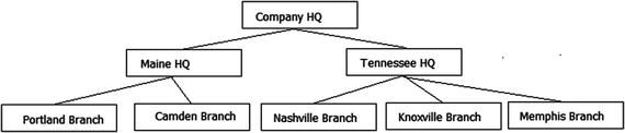
Figure 8-3. Demonstration company hierarchy
The most important thing to understand when dealing with trees in SQL Server is that the most efficient way to work with trees in a procedural language is not the most efficient way to work with data in a set-based relational language. Both use recursion, but the implementation is very different. If you were searching a tree in a functional language, a very common algorithm would be to traverse the tree one node at a time, from the topmost item, down to the lowest in the tree, and then work your way around to all of the nodes. This is generally done using a recursive algorithm, based on the ordering of the items in the tree. In Figure 8-4, I show this for the left side of the tree.

Figure 8-4. Sample tree structure searched depth first
This is referred to as a depth-first search and is fast when the language is optimized for single-instance-at-a-time access, particularly when you can load the entire tree structure into RAM. If you attempted to implement this using T-SQL, you would find that it is obnoxiously slow, as most any iterative processing can be. In SQL, we use what is called a breadth-first search that can be scaled to many more nodes, because the number of queries is limited to the number of levels in the hierarchy. The limitations here pertain to the size of the temporary storage needed and how many rows you end up with on each level. Joining to an unindexed temporary set is bad in your code, and it is not good in SQL Server’s algorithms either.
A tree can be broken down into levels, from the parent row that you are interested in. From there, the levels increase as you are one level away from the parent, as shown in Figure 8-5.
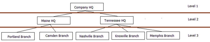
Figure 8-5. Sample tree structure with levels
Now, working with this structure will deal with each level as a separate set, joined to the matching results from the previous level. You iterate one level at a time, matching rows from one level to the next. This reduces the number of queries to use the data down to three, rather than a minimum of eight, plus the overhead of going back and forth from parent to child. In SQL, we will use a recursive CTE (common table expression), where the recursion isn’t based on ordering, but rather the anchor SQL referencing the object it is a part of.
To demonstrate working with adjacency list tables, let’s create a table to represent a hierarchy of companies that are parent to one another. The goal of our table will be to implement the structure, as shown in Figure 8-6.
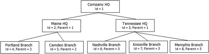
Figure 8-6. Diagram of basic adjacency list
So we will create the following table:
CREATE SCHEMA Corporate;
GO
CREATE TABLE Corporate.Company
(
    CompanyId   int NOT NULL CONSTRAINT PKCompany PRIMARY KEY,
    Name        varchar(20) NOT NULL CONSTRAINT AKCompany_Name UNIQUE,
    ParentCompanyId int NULL
      CONSTRAINT Company$isParentOf$Company REFERENCES Corporate.Company(companyId)
);
Then, load data to set up a table like the graphic in Figure 8-3:
INSERT INTO Corporate.Company (CompanyId, Name, ParentCompanyId)
VALUES (1, ’Company HQ’, NULL),
       (2, ’Maine HQ’,1),              (3, ’Tennessee HQ’,1),
       (4, ’Nashville Branch’,3),      (5, ’Knoxville Branch’,3),
       (6, ’Memphis Branch’,3),        (7, ’Portland Branch’,2),
       (8, ’Camden Branch’,2);
Now, taking a look at the data
SELECT *
FROM    Corporate.Company;
returns the following: