CHAPTER 10
Worksheet Basics
Add a Worksheet
By default, when you create a new blank workbook in Excel, it contains one worksheet, which is often all you need. In some cases, however, your workbook might require additional worksheets. For example, if your workbook contains data about products your company sells, you might want to add worksheets related to the product data, such as calculations, data analysis, charts, or PivotTables.
When you add a new worksheet, Excel gives it a default name. To help you better keep track of your data, you can rename your new worksheet. For more information, see the next section, “Rename a Worksheet.”
Add a Worksheet

![]() Click the New Sheet button (
Click the New Sheet button (![]() ).
).
![]() You can also right-click a worksheet tab, click Insert to open the Insert dialog box, click Worksheet, and then click OK.
You can also right-click a worksheet tab, click Insert to open the Insert dialog box, click Worksheet, and then click OK.
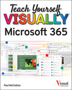
![]() Excel adds a new blank worksheet and gives it a default worksheet name.
Excel adds a new blank worksheet and gives it a default worksheet name.
Rename a Worksheet
When you create a new workbook, Excel assigns the default name Sheet1 to the worksheet. Likewise, Excel assigns default names (Sheet2, Sheet3, and so on) to each worksheet you add to an existing workbook. To help you identify their content, you can change the names of your Excel worksheets to something more descriptive. For example, if your workbook contains four worksheets, each detailing a different sales quarter, then you can give each worksheet a unique name, such as Quarter 1, Quarter 2, and so on.
Rename a Worksheet

![]() Double-click the worksheet tab that you want to rename.
Double-click the worksheet tab that you want to rename.
![]() Excel opens the name for editing and highlights the current name.
Excel opens the name for editing and highlights the current name.
![]() You can also right-click the worksheet name and click Rename.
You can also right-click the worksheet name and click Rename.

![]() Type a new name for the worksheet.
Type a new name for the worksheet.
Note: Worksheet names must be 1 to 31 characters long, must be unique in the workbook, and cannot contain any of the following characters: / ? * : [ or ].
![]() Press
Press ![]() .
.
Excel assigns the new worksheet name.
Change Page Setup Options
You can change worksheet settings related to page orientation, margins, and more. For example, suppose that you want to print a worksheet that has a few more columns than will fit on a page in Portrait orientation. (Portrait orientation accommodates fewer columns but more rows on the page and is the default page orientation that Excel assigns.) You can change the orientation of the worksheet to Landscape, which accommodates more columns but fewer rows on a page.
You can also use Excel’s page setup settings to insert page breaks and set margins to control the placement of data on a printed page.
Change Page Setup Options
Change the Page Orientation
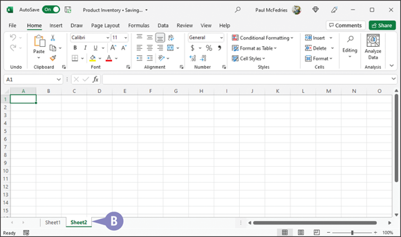
![]() Click the Page Layout tab.
Click the Page Layout tab.
![]() Click Orientation.
Click Orientation.
![]() Click Portrait or Landscape.
Click Portrait or Landscape.
Note: Portrait is the default orientation.
![]() Vertical and horizontal (not shown) dotted lines identify page breaks that Excel inserts after you change the orientation at least once.
Vertical and horizontal (not shown) dotted lines identify page breaks that Excel inserts after you change the orientation at least once.

Excel applies the new orientation. This example applies Landscape.
![]() Excel moves the page break indicators based on the new orientation.
Excel moves the page break indicators based on the new orientation.
![]() You can click the Margins button to set up page margins.
You can click the Margins button to set up page margins.
Insert a Page Break
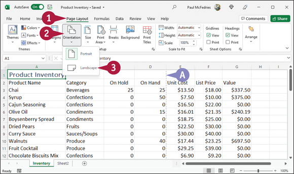
![]() Select a cell in the row above which you want to insert a page break.
Select a cell in the row above which you want to insert a page break.
![]() Click the Page Layout tab.
Click the Page Layout tab.
![]() Click Breaks.
Click Breaks.
![]() Click Insert Page Break.
Click Insert Page Break.

![]() Excel inserts a solid line representing a user-inserted page break.
Excel inserts a solid line representing a user-inserted page break.
Move or Copy Worksheets
You can move or copy a worksheet to a new location within the same workbook or to an entirely different workbook. For example, moving a worksheet is helpful if you insert a new worksheet and the worksheet tab names appear out of order.
Besides moving worksheets, you can also copy them. Copying a worksheet is helpful when you plan to make major changes to the worksheet and you want a backup copy. Or you might want to copy a worksheet if you need a new worksheet that uses much of the same structure or data as an existing worksheet.
Move or Copy Worksheets
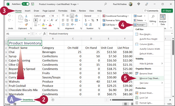
![]() If you plan to move or copy a worksheet to a different workbook, open the other workbook.
If you plan to move or copy a worksheet to a different workbook, open the other workbook.
![]() Click the tab of the worksheet you want to move or copy to make it the active worksheet.
Click the tab of the worksheet you want to move or copy to make it the active worksheet.
![]() Click Home.
Click Home.
![]() Click Format.
Click Format.
![]() Click Move or Copy Sheet.
Click Move or Copy Sheet.
![]() You can also right-click the worksheet tab and then click Move or Copy.
You can also right-click the worksheet tab and then click Move or Copy.
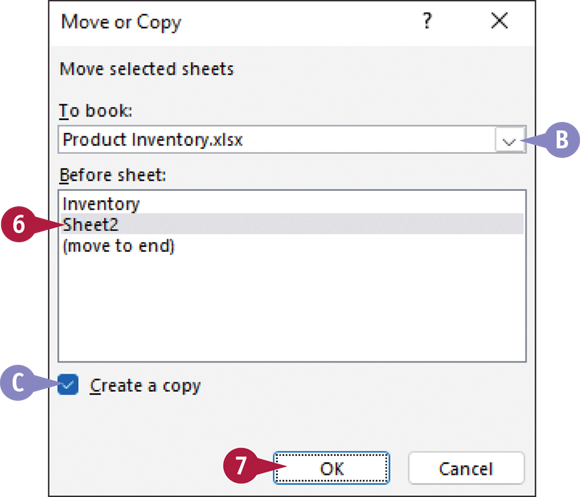
![]() The Move or Copy dialog box appears.
The Move or Copy dialog box appears.
![]() You can click the To book
You can click the To book ![]() to select a destination workbook.
to select a destination workbook.
![]() Click the worksheet before which you want the moved or copied worksheet to appear.
Click the worksheet before which you want the moved or copied worksheet to appear.
![]() You can copy a worksheet by selecting Create a copy (
You can copy a worksheet by selecting Create a copy (![]() changes to
changes to ![]() ).
).
![]() Click OK.
Click OK.
Excel moves or copies the worksheet to the new location.
Delete a Worksheet
You can delete a worksheet that you no longer need. For example, you might delete a worksheet that contains outdated data or information about a product that your company no longer sells.
When you delete a worksheet, Excel prompts you to confirm the deletion unless the worksheet is blank, in which case it deletes the worksheet immediately. When you delete a worksheet, Excel permanently removes it from the workbook and displays the worksheet to the right of the one you deleted unless you deleted the last worksheet. In that case, Excel displays the worksheet to the left of the one you deleted.
Delete a Worksheet
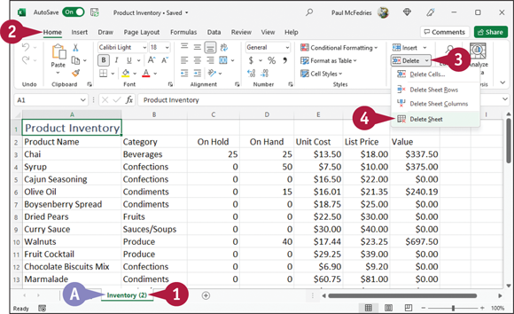
![]() Click the tab of the worksheet you want to delete.
Click the tab of the worksheet you want to delete.
![]() Click Home.
Click Home.
![]() Click the Delete
Click the Delete ![]() .
.
![]() Click Delete Sheet.
Click Delete Sheet.
![]() You can also right-click the worksheet tab and then click Delete.
You can also right-click the worksheet tab and then click Delete.
If the worksheet is blank, Excel deletes it immediately.

If the worksheet contains any data, Excel prompts you to confirm the deletion.
![]() Click Delete.
Click Delete.
Excel deletes the worksheet.
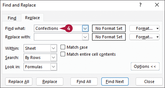
Find and Replace Data
You can search for information in your worksheet and replace it with other information. For example, suppose that you want to change the product category Confections to Sweets. You can search for Confections and replace each occurrence with Sweets. Be aware that Excel finds all occurrences of information as you search and replace it, so be careful when replacing all occurrences at once. You can search and then skip occurrences that you do not want to replace.
You can search the entire worksheet or you can limit the search to a range of cells that you select before you begin the search.
Find and Replace Data

![]() Click the Home tab.
Click the Home tab.
![]() Click Find & Select.
Click Find & Select.
![]() Click Replace.
Click Replace.
![]() To only search for information, click Find instead.
To only search for information, click Find instead.
Excel displays the Replace tab of the Find and Replace dialog box.
![]() Use the Find What text box to type the text that you want to find and replace.
Use the Find What text box to type the text that you want to find and replace.

![]() Use the Replace With text box to type the text that you want Excel to use to replace the text you typed in step 4.
Use the Replace With text box to type the text that you want Excel to use to replace the text you typed in step 4.
![]() Click Find Next.
Click Find Next.

![]() Excel finds the first occurrence of the text.
Excel finds the first occurrence of the text.
![]() Click Replace.
Click Replace.
Excel replaces the information in the cell and finds the next occurrence.
![]() Repeat step 7 as needed.
Repeat step 7 as needed.
![]() If you find an occurrence that you do not want to replace, click Find Next instead.
If you find an occurrence that you do not want to replace, click Find Next instead.
![]() You can click Replace All if you do not want to review each occurrence before Excel replaces it.
You can click Replace All if you do not want to review each occurrence before Excel replaces it.
Excel displays a message when it cannot find any more occurrences.
![]() Click OK (not shown) and then click Close.
Click OK (not shown) and then click Close.
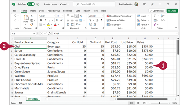
Create a Table
You can create a table from any rectangular range of related data in a worksheet. A table is a collection of related information. Table rows — called records — contain information about one element, and table columns divide the element into fields. In a table containing name and address information, a record would contain all the information about one person, and all first names, last names, addresses, and so on would appear in separate columns.
When you create a table, Excel identifies the information in the range as a table and simultaneously formats the table and adds AutoFilter arrows to each column.
Create a Table
![]() Set up a range in a worksheet that contains similar information for each row.
Set up a range in a worksheet that contains similar information for each row.
![]() Click anywhere in the range.
Click anywhere in the range.

![]() Click Insert.
Click Insert.
![]() Click Table.
Click Table.
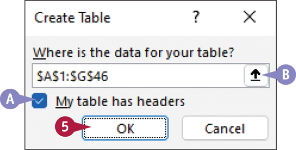
The Create Table dialog box appears, displaying a suggested range for the table.
![]() You can click My table has headers (
You can click My table has headers (![]() changes to
changes to ![]() ) if labels for each column do not appear in the first row of the range.
) if labels for each column do not appear in the first row of the range.
![]() You can click the Range selector button (
You can click the Range selector button (![]() ) to select a new range for the table boundaries by dragging in the worksheet.
) to select a new range for the table boundaries by dragging in the worksheet.
![]() Click OK.
Click OK.
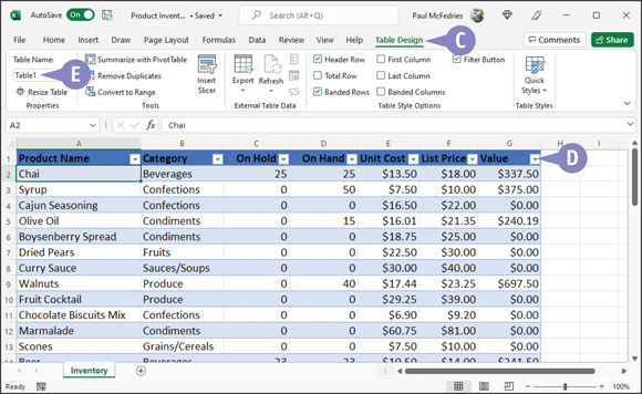
Excel creates a table and applies a table style to it.
![]() The Table Design contextual tab appears on the Ribbon.
The Table Design contextual tab appears on the Ribbon.
![]()
![]() appears in each column header.
appears in each column header.
![]() Excel assigns the table a generic name.
Excel assigns the table a generic name.
Filter or Sort Table Information
When you create a table, Excel automatically adds AutoFilter arrows to each column; you can use these arrows to quickly and easily filter and sort the information in the table.
When you filter a table, you display only those rows that meet conditions you specify, and you specify those conditions by making selections from the AutoFilter lists. You can also use the AutoFilter arrows to sort information in a variety of ways. Excel recognizes the type of data stored in table columns and offers you sorting choices that are appropriate for the type of data.
Filter or Sort Table Information

Filter a Table
![]() Click
Click ![]() next to the column heading you want to use for filtering.
next to the column heading you want to use for filtering.
![]() Excel displays a list of the unique values in the selected column.
Excel displays a list of the unique values in the selected column.
![]() To exclude all instances of a particular value, deselect that value’s check box (
To exclude all instances of a particular value, deselect that value’s check box (![]() changes to
changes to ![]() ).
).
![]() To include all instances of a particular value, select that value’s check box (
To include all instances of a particular value, select that value’s check box (![]() changes to
changes to ![]() ).
).
![]() Repeat steps 2 and 3 until you have selected all the filters you want to use.
Repeat steps 2 and 3 until you have selected all the filters you want to use.
![]() Click OK.
Click OK.
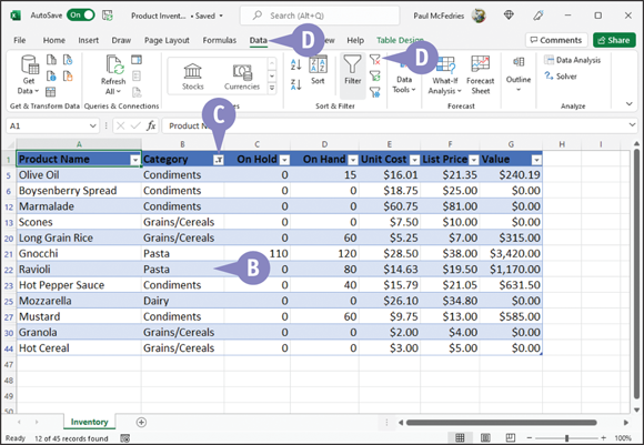
![]() Excel displays only the data meeting the criteria you selected in step 2.
Excel displays only the data meeting the criteria you selected in step 2.
![]() The AutoFilter
The AutoFilter ![]() changes to
changes to ![]() to indicate the data in the column is filtered.
to indicate the data in the column is filtered.
![]() To clear the filter, click Data and then click Clear (
To clear the filter, click Data and then click Clear (![]() ).
).

Sort a Table
![]() Click
Click ![]() next to the column heading you want to use for sorting
next to the column heading you want to use for sorting
![]() Excel displays a list of possible sort orders.
Excel displays a list of possible sort orders.
![]() Click a sort order.
Click a sort order.
This example sorts from largest to smallest.

![]() Excel re-orders the information.
Excel re-orders the information.
![]()
![]() changes to
changes to ![]() to indicate the data in the column is sorted.
to indicate the data in the column is sorted.
Note: You cannot clear a sort the way you can a filter. To remove a sort, you can click Home and then click Undo ![]() .
.
Analyze Data Quickly
You can easily analyze data in a variety of ways using the Quick Analysis button. You can apply various types of conditional formatting; create different types of charts, including line and column charts; or add miniature graphs called sparklines (see Chapter 12 for details on sparkline charts). You can also sum, average, and count occurrences of data as well as calculate percent of total and running total values. In addition, you can apply a table style and create a variety of different PivotTables.
The choices displayed in each analysis category are not always the same; the ones you see depend on the type of data you select.
Analyze Data Quickly

![]() Select a range of data to analyze.
Select a range of data to analyze.
![]() The Quick Analysis button (
The Quick Analysis button (![]() ) appears.
) appears.
![]() Click the Quick Analysis button (
Click the Quick Analysis button (![]() ).
).

Quick Analysis categories appear.
![]() Click each category heading to view the options for that category.
Click each category heading to view the options for that category.
![]() Point the mouse (
Point the mouse (![]() ) at a choice under a category.
) at a choice under a category.
![]() A preview of that analysis choice appears.
A preview of that analysis choice appears.
Note: For an explanation of the Quick Analysis choices, see the next section, “Understanding Data Analysis Choices.”
![]() When you find the analysis choice you want to use, click it and Excel creates it.
When you find the analysis choice you want to use, click it and Excel creates it.
Understanding Data Analysis Choices
The Quick Analysis button (![]() ) offers a variety of ways to analyze selected data. This section provides an overview of the analysis categories and the choices offered in each category.
) offers a variety of ways to analyze selected data. This section provides an overview of the analysis categories and the choices offered in each category.
Formatting
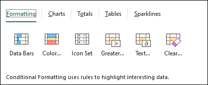
Use formatting to highlight parts of your data. With formatting, you can add data bars, color scales, and icon sets. You can also highlight values that exceed a specified number and cells that contain specified text.
Charts

Pictures often get your point across better than raw numbers. You can quickly chart your data; Excel recommends different chart types, based on the data you select. If you do not see the chart type you want to create, you can click More.
Totals

Using the options in the Totals category, you can easily calculate sums — of both rows and columns — as well as averages, percent of total, and the number of occurrences of the values in the range. You can also insert a running total that grows as you add items to your data.
Tables

Using the choices under the Tables category, you can convert a range to a table, making it easy to filter and sort your data. You can also quickly and easily create a variety of PivotTables — Excel suggests PivotTables you might want to consider and then creates any you might choose.
Sparklines
Sparklines are tiny charts that you can display beside your data that provide trend information for selected data. See Chapter 12 for more information on sparkline charts.

Insert a Note
You can add notes to your worksheets. You might add a note to make a comment or reminder to yourself about a particular cell’s contents, or you might include a note for other users to see. For example, if you share your workbooks with other users, you can use notes to leave feedback about the data without typing directly in the worksheet.
When you add a note to a cell, Excel displays a small red triangle in the upper-right corner of the cell until you choose to view it. Notes you add are identified with your username.
Insert a Note

Add a Note
![]() Click the cell to which you want to add a note.
Click the cell to which you want to add a note.
![]() Click Review.
Click Review.
![]() Click Notes.
Click Notes.
![]() Click New Note.
Click New Note.
You can also right-click the cell and choose Insert Note.

A note balloon appears.
![]() Type your note text.
Type your note text.

![]() Click anywhere outside the note balloon to deselect the note.
Click anywhere outside the note balloon to deselect the note.
![]() Cells that contain notes display a tiny red triangle in the upper-right corner.
Cells that contain notes display a tiny red triangle in the upper-right corner.

View a Note
![]() Position the mouse (
Position the mouse (![]() ) over a cell containing a note.
) over a cell containing a note.
![]() The note balloon appears, displaying the note.
The note balloon appears, displaying the note.