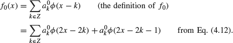
4
HAAR WAVELET ANALYSIS
Wavelets were first applied in geophysics to analyze data from seismic surveys, which are used in oil and mineral exploration to get “pictures” of layering in subsurface rock. In fact, geophysicists rediscovered them; mathematicians had developed them to solve abstract problems some 20 years earlier, but had not anticipated their applications in signal processing.1
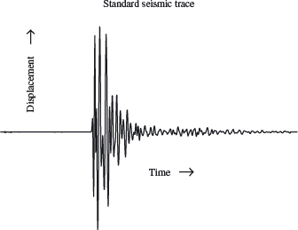
Seismic surveys are made up of many two-dimensional pictures or slices. These are sewn together to give a three-dimensional image of the structure of rock below the surface. Each slice is obtained by placing geophones–seismic “microphones”–at equally spaced intervals along a line, the seismic line. Dynamite is set off at one end of the line to create a seismic wave in the ground. Every geophone along the line records the movement of the earth due to the blast, from start to finish; this record is its seismic trace (see Figure 4.1).
The first wave recorded by the geophones is the direct wave, which travels along the surface. This is usually not important. Subsequent waves are reflected off rock layers below ground. These are the important ones. Knowledge of the time that the wave hits a geophone gives information about where the layer that reflected it is located. The “wiggles” that the wave produces tell something about the fine details of the layer. The traces from the all the geophones on a line can be combined to give the slice for the ground directly beneath the line.
Figure 4.1. The figure shows a typical seismic trace. Displacement is plotted versus time. Both the oscillations and the time they occur are important.
The key to an accurate seismic survey is proper analysis of each trace. The Fourier transform is not a good tool here. It can only provide frequency information (the oscillations that comprise the signal). It gives no direct information about when an oscillation occurred. Another tool, the short-time Fourier transform, is better. The full time interval is divided into a number of small, equal time intervals; these are individually analyzed using the Fourier transform. The result contains time and frequency information. However, there is a problem with this approach. The equal time intervals are not adjustable; the times when very short duration, high-frequency bursts occur are hard to detect.
Enter wavelets. Wavelets can keep track of time and frequency information. They can be used to “zoom in” on the short bursts mentioned previously, or to “zoom out” to detect long, slow oscillations.
4.2.1 The Haar Scaling Function
There are two functions that play a primary role in wavelet analysis: the scaling function ϕ and the wavelet ψ. These two functions generate a family of functions that can be used to break up or reconstruct a signal. To emphasize the “marriage” involved in building this “family,” ϕ is sometimes called the “father wavelet,” and ψ is sometimes referred to as the “mother wavelet.”
Figure 4.2. Graph of the Haar scaling function.
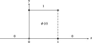
The simplest wavelet analysis is based on the Haar scaling function, whose graph is given in Figure 4.2. The building blocks are translations and dilations (both in height and width) of this basic graph.
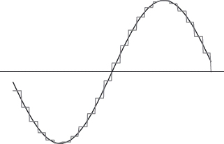
We want to illustrate the basic ideas involved in such an analysis. Consider the signal shown in Figure 4.3. We may think of this as a measurement of some physical quantity–perhaps line voltage over a single cycle–as a function of time. The two sharp spikes in the graph might represent noise coming from a loose connection in the volt meter, and we want to filter out this undesirable noise. The graph in Figure 4.4 shows one possible approximation to the signal using Haar building blocks. The high-frequency noise shows up as tall thin blocks. An algorithm that deletes the thin blocks will eliminate the noise and not disturb the rest of the signal.
Figure 4.3. Voltage from a faulty meter.
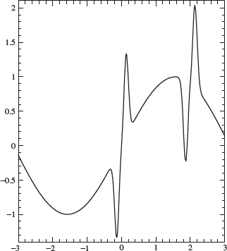
Figure 4.4. Approximation of voltage signal by Haar functions.
The building blocks generated by the Haar scaling function are particularly simple and they illustrate the general ideas underlying a multiresolution analysis, which we will discuss in detail. The disadvantage of the Haar wavelets is that they are discontinuous and therefore do not approximate continuous signals very well (Figure 4.4 does not really approximate Figure 4.3 too well). In later sections we introduce other wavelets, due to Daubechies, that are continuous but still retain the localized behavior exhibited by the Haar wavelets.
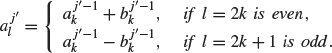
Definition 4.1 The Haar scaling function is defined as
![]()
The graph of the Haar scaling function is given in Figure 4.2.
Figure 4.5. Graph of typical element in V0
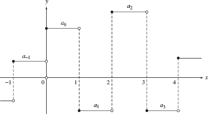
The function ϕ (x − k) has the same graph as ϕ but is translated to the right by k units (assuming k is positive). Let V0 be the space of all functions of the form
![]()
where k can range over any finite set of positive or negative integers. Since ϕ (x – k) is discontinuous at x = k and x = k + 1, an alternative description of V0 is that it consists of all piecewise constant functions whose discontinuities are contained in the set of integers. Since k ranges over a finite set, each element of V0 is zero outside a bounded set. Such a function is said to have finite or compact support. The graph of a typical element of V0 is given in Figure 4.5. Note that a function in V0 may not have discontinuities at all the integers (for example, if a1 = a2, then the previous sum is continuous at x = 2).
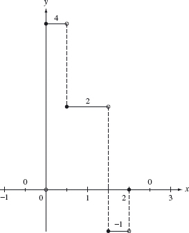
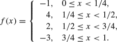
Example 4.2 The graph of the function
![]()
is given in Figure 4.6. This function has discontinuities at x = 0,1, 3, and 4.
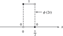
We need blocks that are thinner to analyze signals of high frequency. The building block whose width is half that of the graph of ϕ is given by the graph of ϕ (2x) shown in Figure 4.7.
The function ϕ (2x – k) = ϕ (2(x – k/2)) is the same as the graph of the function of ϕ (2x) but shifted to the right by k/2 units. Let V1 be the space of functions of the form
Figure 4.6. Plot of ƒ in Example 4.2.
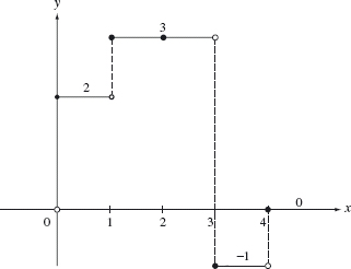
Figure 4.7. Graph of ϕ(2x)
![]()
Geometrically, V1 is the space of piecewise constant functions of finite support with possible discontinuities at the half integers {0, ±1/2, ±1, ±3/2...}.
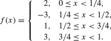
Example 4.3 The graph of the function
![]()
is given in Figure 4.8. This function has discontinuities at x = 0,1/2, 3/2, and 2.
We make the following more general definition.
Figure 4.8. Plot of f in Example 4.3.
Definition 4.4 Suppose j is any nonnegative integer. The space of step functions at level j, denoted by Vj, is defined to be the space spanned by the set
![]()
over the real numbers. Vj is the space of piecewise constant functions of finite support whose discontinuities are contained in the set
![]()
A function in V0 is a piecewise constant function with discontinuities contained in the set of integers. Any function in V0 is also contained in V1,which consists of piecewise constant functions whose discontinuities are contained in the set of half integers {... – 1/2, 0, 1/2, 1, 3/2...}. Likewise, V1 ⊂ V2 and so forth:
![]()
This containment is strict. For example, the function ϕ(2x) belongs to V1 but does not belong to V0 (since ϕ(2x) is discontinuous at x = 1/2).
Vj contains all relevant information up to a resolution scale of order 2–j As j gets larger, the resolution gets finer. The fact that Vj ⊂ Vj+1 means that no information is lost as the resolution gets finer. This containment relation is also the reason why Vj is defined in terms of ϕ(2jx) instead of ϕ(ax) for some other factor a. If, for example, we had defined V2 using ϕ(3x – j) instead of ϕ(4x – j), then V2 would not contain V1(since the set of multiples of 1/2 is not contained in the set of multiples of 1/3).
4.2.2 Basic Properties of the Haar Scaling Function
The following theorem is an easy consequence of the definitions.
Theorem 4.5
- A function f(x) belongs to V0 if and only if f(2jx) belongs to Vj.
- A function f(x) belongs to Vj if and only if f(2–jx) belongs to V0.
Proof. To prove the first statement, if a function f belongs to V0 then f(x) is a linear combination of {ϕ(x – k), k ∈ Z}. Therefore, f(2jx) is a linear combination of {ϕ(2jx – k), k ∈ Z}, which means that f(2jx) is a member of Vj. The proofs of the converse and the second statement are similar.
The graph of the function ϕ(2jx) is a spike of width 1/2j. When j is large, the graph of ϕ(2jx) (appropriately translated) is similar to one of the spikes of a signal that we may wish to filter out. Thus it is desirable to have an efficient algorithm to decompose a signal into its Vj components. One way to perform this decomposition is to construct an orthonormal basis for Vj (using the L2 inner product).
Let’s start with V0. This space is generated by ϕ and its translates. The functions ϕ(x – k) each have unit norm in L2, that is,
![]()
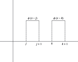
If j is different from k, then ϕ(x – j) and ϕ(x – k) have disjoint supports (see Figure 4.9). Therefore
![]()
and so the set {ϕ(x – k),k ∈ Z} is an orthonormal basis for V0.
The same argument establishes the following more general result.
Theorem 4.6 The set of functions {2j/2ϕ(2Jx – k); k ∈ Z} is an orthonormal basis of Vj
![]()
Figure 4.9. ϕ(x – j) and ϕ(x – k) have disjoint support.
4.2.3 The Haar Wavelet
Having an orthonormal basis of Vj is only half of the picture. In order to solve our noise filtering problem, we need to have a way of isolating the “spikes” which belong to Vj but which are not members of Vj–1. This is where the wavelet ψ enters the picture.
The idea is to decompose Vj as an orthogonal sum of Vj–1 and its complement. Again, let’s start with j = 1 and identify the orthogonal complement of V0 in V1. Since V0 is generated by ϕ and its translates, it is reasonable to expect that the orthogonal complement of V0 is generated by the translates of some function ψ. Two key facts are needed to construct ψ.
1. ψ is a member of V1and so ψ can be expressed as ψ(x) = ∑l alϕ(2x – l) for some choice of al ∈ R (and only a finite number of the al are non-zero).
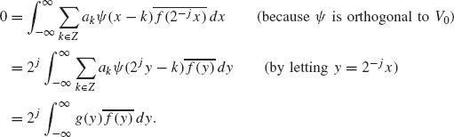
2. ψ is orthogonal to V0. This is equivalent to ∫ ψ (x)ϕ(x – k) dx =0 for all integers k.
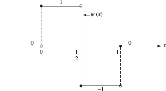
The first requirement means that ψ is built from blocks of width 1/2—that is, scalar multiples of Figure 4.7 and its translates. The second requirement with k = 0 implies ![]() ψ(x)ϕ(x) dx = 0. The simplest ψ satisfying both of these requirements is the function whose graph appears in Figure 4.10. This graph consists of two blocks of width one-half and can be written as
ψ(x)ϕ(x) dx = 0. The simplest ψ satisfying both of these requirements is the function whose graph appears in Figure 4.10. This graph consists of two blocks of width one-half and can be written as
![]()
Figure 4.10. The Haar wavelet ψ(x).
thus satisfying the first requirement. In addition, we have
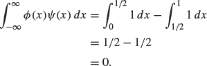
Thus, ψ is orthogonal to ϕ. If k ≠ 0, then the support of ψ(x) and the support of ϕ(x – k) do not overlap and so ∫ψ(x)ϕ(x – k) dx = 0. Therefore, ifr belongs to V1 and is orthogonal to V0; ψ is called the Haar wavelet.
Definition 4.7 The Haar wavelet is the function
![]()
Its graph is given in Figure 4.10.
You can show (see exercise 5) that any function
![]()
is orthogonal to V0 (i.e., orthogonal to each ϕ(x – l), l ∈ Z) if and only if
![]()
In this case,
In other words, a function in V1 is orthogonal to V0 if and only if it is of the form ∑kakψ(x – k) (relabeling a2K by ak).
Let W0 be the space of all functions of the form
![]()
where, again, we assume that only a finite number of the ak are nonzero. What we have just shown is that W0 is the orthogonal complement of V0 in V1; in other words, V1 = V0 ⊕ W0 (recall from Chapter 0 that ⊕ means that V0 and W0 are orthogonal to each other).
In a similar manner, the following, more general result can be established.
Theorem 4.8 Let Wj be the space of functions of the form
![]()
where we assume that only a finite number of ak are nonzero. Wj is the orthogonal complement of Vj in Vj+1 and
![]()
Proof. To establish this theorem, we must show two facts:
1. Each function in Wj is orthogonal to every function in Vj).
2. Any function in Vj+1 which is orthogonal to Vj must belong to Wj.
For the first requirement, suppose that g = ∑k∈Z akψ(2jx – k) belongs to Wj and suppose f belongs to Vj. We must show
![]()
Since f (x) belongs to Vj, the function f (2–j x) belongs to V0. So
Therefore, g is orthogonal to any f ∈ Vj and the first requirement has been established.
The discussion leading to Eq. (4.1) establishes the second requirement when j = 0 since we showed that any function in V1 which is orthogonal to V0 must be a linear combination of {ψ(x – k), k ∈ Z}. The case for general j is analogous to the case when j = 0.
By successively decomposing Vj, Vj–1, and so on, we have
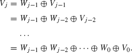
So each f in Vj can be decomposed uniquely as a sum
![]()
where each wl belongs to Wl, 0 ≤ l ≤ j – 1 and f0 belongs to V0. Intuitively, wl represents the “spikes” of f of width 1/2l+1 that cannot be represented as linear combinations of spikes of other widths.
What happens when j goes to infinity? The answer is provided in the following theorem.
Theorem 4.9 The space L2(R) can be decomposed as an infinite orthogonal direct sum
![]()
In particular, each f ∈ L2(R) can be written uniquely as
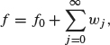
where f0 belongs to V0 and wj belongs to Wj.
The infinite sum should be thought of as a limit of finite sums. In other words,
(4.2)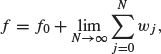
where the limit is taken in the sense of L2. Although the proof of this result is beyond the scope of this text, some intuition can be given. There are two key ideas. The first is that any function in L2(R) can be approximated by continuous functions (for an intuitive explanation of this idea, see Lemma 1.38). The second is that any continuous function can be approximated as closely as desired by a step function whose discontinuities are multiples of 2–j for suitably large j (see Figure 4.11). Such a step function, by definition, belongs to Vj. The theorem is then established by putting both ideas together.
Figure 4.11. Approximating by step functions.
4.3 HAAR DECOMPOSITION AND RECONSTRUCTION ALGORITHMS
4.3.1 Decomposition
Now that Vj has been decomposed as a direct sum of V0 and Wl for 0 ≤ l < j, the solution to our noise filtering problem is theoretically easy. First, we approximate f by a step function fj ∈ Vj (for j suitably large) using Theorem 4.9. Then we decompose fj into its components
![]()
The component, wl, represents a “spike” of width 1/2l+1. For l sufficiently large, these spikes are thin enough to represent noise. For example, suppose that spikes of width less than .01 represent noise. Since 2–6 > .01 > 2–7, any wj with j ≥ 6 represents noise. To filter out this noise, these components can be set equal to zero. The rest of the sum represents a signal that is still relatively close to f and which is noise free.
In order to implement this theoretical algorithm, an efficient way of performing the decomposition given in Theorem 4.9 is needed. The first step is to approximate the original signal f by a step function of the form
(4.3)![]()
The procedure is to sample the signal at x = ... – 1/2j, 0, 1/2j,..., which leads to al = f(l/2j) for l ∈ Z. An illustration of this procedure is given in Figure 4.11, where f is the continuous signal and fj, is the step function. Here, j is chosen so that the mesh size 2–j is small enough so that fj(x) captures the essential features of the signal. The range of l depends on the domain of the signal. If the signal is defined on 0 ≤ x ≤ 1, then the range of l is 0 ≤ l ≤ 2j – 1. In general, we will not specify the range of / unless a specific example is discussed.
Now, the task is to decompose ϕ(2 jx – l) into its Wl components for l < j. The following relations between ϕ and ψ are needed.
(4.4)![]()
(4.5)![]()
which follow easily by looking at their graphs (see Figures 4.2 and 4.10). More generally, we have the following lemma.
Lemma 4.10 The following relations hold for all x ∈ R.
(4.6)![]()
(4.7)![]()
This lemma follows by replacing x by 2 j–1x in Eqs. (4.4) and (4.5).
This lemma can be used to decompose ϕ(2j x – l) into its Wl components for l < j. An example will help illustrate the process.
Example 4.11 Let f be given by the graph in Figure 4.12. Notice that the mesh size needed to capture all the features of f is 2 –2. A description of f in terms of ϕ(22 x – l) is given by
We wish to decompose f into its W1, W0, and V0 components. The following equations follow from Eqs. (4.6) and (4.7) with j = 2.
Using these equations together with Eq. (4.8) and collecting terms yield
Figure 4.12. Graph of Example 4.11.
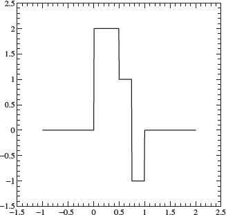
The W1 component of f (x) is ψ(2x – 1), since W1 is the linear span of {ψ(2x – k); k ∈ Z}. The V1 component of f (x) is given by 2ϕ(2x). This component can be further decomposed into a V0 component and a W0 component by using the equation ϕ(2x) = (ϕ(x) + ψ(x))/2. The result is
![]()
This equation can also be verified geometrically by examining the graphs of the functions involved. The terms in the expression at right are the components of f in W1, W0, and V0, respectively.
Using this example as a guide, we can proceed with the general decomposition scheme as follows. First divide up the sum ![]() into even and odd terms:
into even and odd terms:
Next, we use Eqs. (4.6) and (4.7) with x replaced by x – k21 – j:
(4.10)![]()
(4.11)![]()
Substituting these expressions into Eq. (4.9) yields
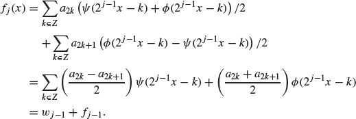
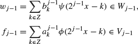
The first term on the right, ![]() j–1, represents the Wj–1 component of fj, since Wj–1 is, by definition, the linear span of {ψ(2j–1 x -k), k ∈ Z}. Likewise, the second term on the right, fj-1, represents the Vj–1 component of fj. We summarize the preceding decomposition algorithm in the following theorem.
j–1, represents the Wj–1 component of fj, since Wj–1 is, by definition, the linear span of {ψ(2j–1 x -k), k ∈ Z}. Likewise, the second term on the right, fj-1, represents the Vj–1 component of fj. We summarize the preceding decomposition algorithm in the following theorem.
Theorem 4.12 (Haar Decomposition) Suppose
![]()
Then fj can be decomposed as
![]()
where
with
![]()
The preceding process can now be repeated with j replaced by j – 1 to decompose fj–1 as ![]() j–2 + fj–2. Continuing in this way, we achieve the decomposition
j–2 + fj–2. Continuing in this way, we achieve the decomposition
![]()
To summarize the decomposition process, a signal is first discretized to produce an approximate signal fj ∈ Vj as in Theorem 4.9. Then the decomposition algorithm in Theorem 4.12 produces a decomposition of fj into its various frequency components: fj = ![]() j–1 +
j–1 + ![]() j–2 +
j–2 + ![]() 0 + f0.
0 + f0.
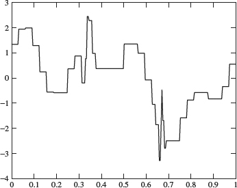
Figure 4.13. Sample signal.
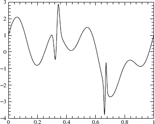
Example 4.13 Consider the signal, f, defined on the unit interval 0 ≤ x ≤ 1 given in Figure 4.13. We discretize this signal over 28 nodes (so ![]() = f(k/28)) since a mesh size of width 1/28 seems to capture the essential features of this signal. Thus
= f(k/28)) since a mesh size of width 1/28 seems to capture the essential features of this signal. Thus
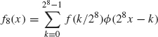
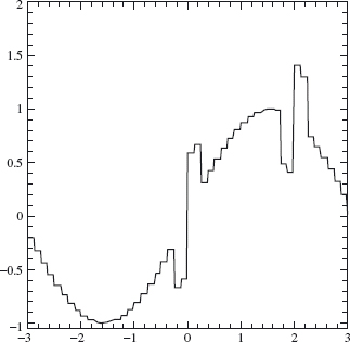
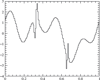
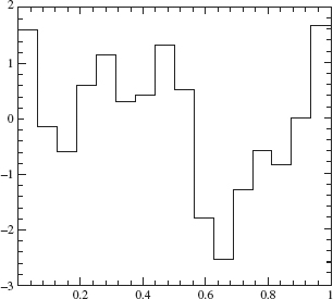
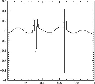
approximates f well enough for our purposes. Using Theorem 4.12, we decompose f8 into its components in Vj, for j = 8, 7, ..., 0. Plots of the components in f8 ∈ V8, f7 ∈ V7, f6 ∈ V6, and f4 ∈ V4 are given in Figures 4.14, 4.15, 4.16 and 4.17. A plot of the W7 component is given in Figure 4.18. The W7 component is small except where the original signal contains a sharp spike of width ≈ 2–8 (at x ≈ 0.3 and x ≈ 0.65).
4.3.2 Reconstruction
Having decomposed f into its V0 and Wj′ components for 0 ≤ j′ < j, then what? The answer depends on the goal. If the goal is to filter out noise, then the Wj′ components of f corresponding to the unwanted frequencies can be thrown out and the resulting signal will have much less noise. If the goal is data compression, the Wj′ components that are small can be thrown out, without appreciably changing the signal. Only the significant Wj′ components (the larger ![]() ) need to be stored or transmitted and significant data compression can be achieved. Of course, what constitutes “small” depends on the tolerance for error for a particular application.
) need to be stored or transmitted and significant data compression can be achieved. Of course, what constitutes “small” depends on the tolerance for error for a particular application.
Figure 4.14. V8 component.
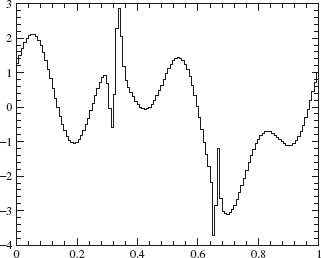
Figure 4.15. V7 component.
In either case, since the ![]() have been modified, we need a reconstruction algorithm (for the receiving end of the signal perhaps) so that the compressed or filtered signal can be rebuilt in terms of the basis elements ϕ (2j x – l) of Vj; that is,
have been modified, we need a reconstruction algorithm (for the receiving end of the signal perhaps) so that the compressed or filtered signal can be rebuilt in terms of the basis elements ϕ (2j x – l) of Vj; that is,
![]()
Figure 4.16. V6 component.
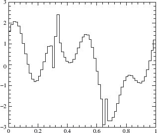
Figure 4.17. V4 component.
Once this is done, the graph of the signal f is a step function of height ![]() over the interval l/2 j ≤ x ≤ (l + 1)/2 j.
over the interval l/2 j ≤ x ≤ (l + 1)/2 j.
We start with a signal of the form
![]()
Figure 4.18. W7 component.
where
![]()
for 0 ≤ l ≤ j – 1. Our goal is to rewrite f as f (x) = ![]() and find an algorithm for the computation of the constants
and find an algorithm for the computation of the constants ![]() . We use the equations
. We use the equations
which follow from the definitions of ϕ and ψ Replacing x by 2 j–1x yields
(4.14)![]()
(4.15)![]()
Using Eq. (4.12) with x replaced by x – k, we have
So
where
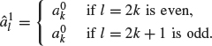
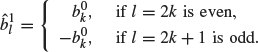
Similarly, ![]() can be written [using Eq. (4.13) for ψ(x – k)] as
can be written [using Eq. (4.13) for ψ(x – k)] as
where
Combining Eqs. (4.16) and (4.17) yields
![]()
where
![]()
Next, ![]() is added to this sum in the same manner [using Eqs. (4.12) and (4.13) with x replaced by 2x – k]:
is added to this sum in the same manner [using Eqs. (4.12) and (4.13) with x replaced by 2x – k]:
![]()
where
![]()
Note that the ![]() and
and ![]() coefficients determine the
coefficients determine the ![]() coefficients. Then, the
coefficients. Then, the ![]() and
and ![]() coefficients determine the
coefficients determine the ![]() coefficients, and so on, in a recursive manner.
coefficients, and so on, in a recursive manner.
The preceding reconstruction algorithm is summarized in the following theorem.
Theorem 4.14 (Haar Reconstruction) If f = f 0 + ![]() 0 +
0 + ![]() 1 +
1 + ![]() 2 + ... +
2 + ... + ![]() j–1 with
j–1 with
![]()
for 0 ≤ j′ < j, then
![]()
where the ![]() are determined recursively for j′ = 1, then j′ = 2 ... until j′ = j by the algorithm
are determined recursively for j′ = 1, then j′ = 2 ... until j′ = j by the algorithm
Example 4.15 We apply the decomposition and reconstruction algorithms to compress the signal f that is shown in Figure 4.19; f is defined on the unit interval. (This is the same signal used in Example 4.13.)
We discretize this signal over 28 nodes (so ![]() = f (k/28)) and then decompose this signal (as in Theorem 4.12) to obtain f = f 0 +
= f (k/28)) and then decompose this signal (as in Theorem 4.12) to obtain f = f 0 + ![]() 0 +
0 + ![]() 1 +
1 + ![]() 2 + ... +
2 + ... + ![]() 7
7
Figure 4.19. Sample signal.
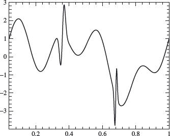
Figure 4.20. Graph showing 80% compression.
with
![]()
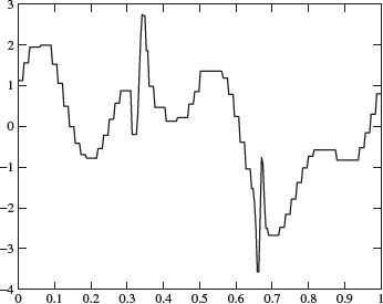
for 0 ≤ j′ ≤ 7. Note that there is only one basis term ϕ (x) in V0 since the interval of consideration is 0 ≤ x ≤ 1. We first use 80% compression on this decomposed signal, which means that after ordering the ![]() by size, we set the smallest 80% equal to zero (retaining the largest 20%). Then we reconstruct the signal as in Theorem 4.14. The result is graphed in Figure 4.20. Figure 4.21 illustrates the same process with 90% compression. The relative L2 error is 0.0895 for 80% compression and 0.1838 for 90% compression.
by size, we set the smallest 80% equal to zero (retaining the largest 20%). Then we reconstruct the signal as in Theorem 4.14. The result is graphed in Figure 4.20. Figure 4.21 illustrates the same process with 90% compression. The relative L2 error is 0.0895 for 80% compression and 0.1838 for 90% compression.
4.3.3 Filters and Diagrams
The decomposition and reconstruction algorithms can be put in the language of discrete filters and simple operators acting on a sequence of coefficients. The algorithms can then be visualized in terms of block diagrams.
We will do the decomposition algorithm first. Define two discrete filters (convolution operators) H and L via their impulse responses, which are the sequences h and ![]() :
:
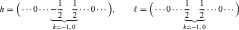
Figure 4.21. Graph showing 90% compression.
If {xk} ∈ ![]() 2, then H(x) := h * x and L(x) :=
2, then H(x) := h * x and L(x) := ![]() * x. The resulting sequences are
* x. The resulting sequences are
![]()
If we keep only even subscripts, then H(x)2k = (h * x)2k = ![]() and L(x)2k = (
and L(x)2k = (![]() * x)2k =
* x)2k = ![]() This operation of discarding the odd coefficients in a sequence is called down sampling ; we will denote the corresponding operator by D.
This operation of discarding the odd coefficients in a sequence is called down sampling ; we will denote the corresponding operator by D.
We now apply these ideas to go from level j scaling coefficients ![]() to get the level j – 1 scaling and wavelet coefficients. Using Theorem 4.12 and replacing x by
to get the level j – 1 scaling and wavelet coefficients. Using Theorem 4.12 and replacing x by ![]() ,
,
![]()
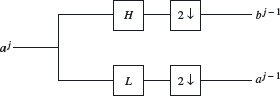
Figure 4.22 illustrates the decomposition algorithm. The down-sampling operator D is replaced by the more suggestive symbol, “2↓.”
The reconstruction algorithm also requires defining two discrete filters ![]() and
and ![]() via their corresponding impulse responses,
via their corresponding impulse responses,
![]()
for a sequence {xk}, we have ![]() = xk – xk–1 and
= xk – xk–1 and ![]() = xk + xk–1. Here is an important observation. If x and y are sequences in which the odd
= xk + xk–1. Here is an important observation. If x and y are sequences in which the odd
Figure 4.22. Haar decomposition diagram.
entries are all 0, then
![]()
Adding the two sequences ![]() *x and
*x and ![]() *y then gives us
*y then gives us
![]()
This is almost the pattern for the reconstruction formula given in Theorem 4.14. Although the x2k+1’s and y2k+1’s are 0, the x2k’s and y2k’s are ours to choose, so we set x2k = ![]() and y2k =
and y2k = ![]() ; that is,
; that is,
![]()
(all odd entries are zero) and similarly for y. The sequences x and y are called up samples of the sequences bj–1 and aj–1. We use the U to denote the up-sampling operator, so x = Ub j–1 and y = Ua j–1. The reconstruction formula then takes the compact form
![]()
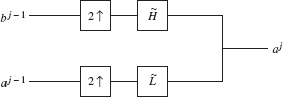
We illustrate the reconstruction step in Figure 4.23. The up-sampling operator is replaced by the symbol 2 ↑.
Figure 4.23. Haar reconstruction diagram.
In this section, we present a summary of the ideas of this chapter. The format is a step-by-step procedure used to process (compress or denoise) a given signal y = f (t). We will let ϕ and ψ be the Haar scaling function and wavelet.
Step 1. Sample. If the signal is continuous (analog), y = f (t), where t represents time, choose the top level j = J so that 2J is larger than the Nyquist rate for the signal (see the discussion just before Theorem 2.23). Let
![]()
In practice, the range of k is a finite interval determined by the duration of the signal. For example, if the duration of the signal is 0 ≤ t ≤ 1, then the range for k is 0 ≤ k ≤ 2J – 1 (or perhaps 1 ≤ l ≤ 2J). If the signal is discrete to start with (i.e., a sequence of numbers), then this step is unnecessary. The top level ![]() is set equal to the kth term in the sampled signal, and 2J is taken to be the sampling rate. In any case, we have the highest-level approximation to f given by
is set equal to the kth term in the sampled signal, and 2J is taken to be the sampling rate. In any case, we have the highest-level approximation to f given by
![]()
Step 2. Decomposition. The decomposition algorithm decomposes fJ into
![]()
where
The coefficients, ![]() and
and ![]() are determined from the a j recursively by the algorithm
are determined from the a j recursively by the algorithm
(4.18)![]()
(4.19)![]()
where H and L are the high- and low-pass filters from Section 4.3.3. When j = J, ![]() and
and ![]() are determined by
are determined by ![]() , which are the sampled signal values from Step 1. Then j becomes J – 1 and
, which are the sampled signal values from Step 1. Then j becomes J – 1 and ![]() and
and ![]() are determined from
are determined from ![]() . Then j becomes J – 2, and so on, until either the level reached is satisfactory for some purpose or there are too few coefficients to continue. Unless otherwise stated, the decomposition algorithm will continue until the j = 0 level is reached, that is,
. Then j becomes J – 2, and so on, until either the level reached is satisfactory for some purpose or there are too few coefficients to continue. Unless otherwise stated, the decomposition algorithm will continue until the j = 0 level is reached, that is,
![]()
Step 3. Processing. After decomposition, the signal is now in the form
(4.20)
(4.21)
The signal can now be filtered by modifying the wavelet coefficients ![]() How this is to be done depends on the problem at hand. To filter out all high frequencies, all the
How this is to be done depends on the problem at hand. To filter out all high frequencies, all the ![]() would be set to zero for j above a certain value. Perhaps only a certain segment of the signal corresponding to particular values of k is to be filtered. If data compression is the goal, then the
would be set to zero for j above a certain value. Perhaps only a certain segment of the signal corresponding to particular values of k is to be filtered. If data compression is the goal, then the ![]() that are below a certain threshold (in absolute value) would be set to zero. Whatever the goal, the process modifies the
that are below a certain threshold (in absolute value) would be set to zero. Whatever the goal, the process modifies the ![]() .
.
Step 4. Reconstruction. Now the goal is to take the modified signal, fJ, in the form (4.21) (with the modified ![]() ) and reconstruct it as
) and reconstruct it as
(4.22)![]()
This is accomplished by the reconstruction algorithm discussed in Section 4.3.3:
(4.23)![]()
for j = 1 ,..., J. When j = 1, the ![]() are computed from the
are computed from the ![]() and
and ![]() When j = 2, the
When j = 2, the ![]() are computed from the
are computed from the ![]() and
and ![]() and so forth. The range of k is determined by the time duration of the signal. When j = J (the top level),
and so forth. The range of k is determined by the time duration of the signal. When j = J (the top level), ![]() represents the approximate value of the processed signal at time x = k/2J. Of course, these
represents the approximate value of the processed signal at time x = k/2J. Of course, these ![]() are different from the original
are different from the original ![]() due the modification of coefficients in Step 3.
due the modification of coefficients in Step 3.
1. Let ϕ and ψ be the Haar scaling and wavelet functions, respectively. Let Vj and Wj be the spaces generated by ϕ (2 ix – k), k ∈ Z, and ψ(2 jx – k), k ∈ Z, respectively. Consider the function defined on 0 ≤ x < 1 given by
Express f first in terms of the basis for V2 and then decompose f into its component parts in W1, W0, and V0. In other words, find the Haar wavelet decomposition for f. Sketch each of these components.
2. Repeat exercise 1 for the function
3. If A and B are finite-dimensional, orthogonal subspaces of an inner product space V, then show
![]()
If A and B are not necessarily orthogonal, then what is the relationship between dim(A + B), dimA, and dimB?
4. (a) Let Vn be the spaces generated by ϕ (2nx – k), k ∈ Z, where ϕ is the Haar scaling function. On the interval 0 ≤ x < 1, what are the dimensions of the spaces Vn and Wn for n ≥ 0 (just count the number of basis elements)?
(b) Using the result of problem 3, count the dimension of the space on the right side of the equality
![]()
Is your answer the same as the one you computed for dimVn in part (a)?
5. Let ϕ and ψ be the Haar scaling and wavelet functions, respectively. Let Vj and Wj be the spaces generated by ϕ (2j x – k), k ∈ Z, and ψ (2j x – k), k ∈ Z, respectively. Suppose f(x) =![]() (ak ∈ R) belongs to V1. Show explicitly that if f is orthogonal to each basis element ϕ (x – l) ∈ V0, for all integers l, then a2l+1 = –a2l for all integers l and hence show
(ak ∈ R) belongs to V1. Show explicitly that if f is orthogonal to each basis element ϕ (x – l) ∈ V0, for all integers l, then a2l+1 = –a2l for all integers l and hence show
![]()
6. Reconstruct g ∈ V3, given these coefficients in its Haar wavelet decomposition:
![]()
The first entry in each list corresponds to k = 0. Sketch g.
7. Reconstruct h ∈ V3 over the interval 0 ≤ x ≤ 1, given the following coefficients in its Haar wavelet decomposition:
![]()
The first entry in each list corresponds to k = 0. Sketch h. The remaining problems require some programming in a language such as MATLAB, Maple, or C. The code in Appendix C may be useful.
8. (Haar wavelets on [0, 1]). Let n be a positive integer, and let f be a continuous function defined on [0, 1]. Let hk(t) = ![]() where ϕ (t) is the Haar scaling function (which is 1 on the interval [0, 1) and zero elsewhere). Form the L2 projection of f onto the span of the hk’s,
where ϕ (t) is the Haar scaling function (which is 1 on the interval [0, 1) and zero elsewhere). Form the L2 projection of f onto the span of the hk’s,
![]()
Show that fn converges uniformly to f on [0, 1]. For f (t) = 1 – t2, use MATLAB or Maple to find the Haar wavelet decomposition on [0, 1] for n = 4, 8, and 16. Plot the results.
9. Let
![]()
Discretize the function f over the interval 0 ≤ t ≤ 1 as described in Step 1 of Section 4.4. Use n = 8 as the top level (so there are 28 nodes in the discretization). Implement the decomposition algorithm described in Step 2 of Section 4.4 using the Haar wavelets. Plot the resulting levels, fj–1 ∈ Vj–1 for j = 8 ... 1 and compare with the original signal.
10. (Continuation of exercise 9). Filter the wavelet coefficients computed in exercise 9 by setting to zero any wavelet coefficient whose absolute value is less than tol = 0.1. Then reconstruct the signal as described in Section 4.4. Plot the reconstructed f8 and compare with the original signal. Compute the relative l2 difference between the original signal and the compressed signal. Experiment with various tolerances. Keep track of the percentage of wavelet coefficients that have been filtered out.
11. Haar wavelets can be used to detect a discontinuity in a signal. Let g(t) be defined on 0 ≤ t < 1 via
Discretize the function g over the interval 0 ≤ t ≤ 1 as described in Step 1 of Section 4.4. Use n = 7 as the top level (so there are 27 nodes in the discretization). Implement a 1-level decomposition. Plot the magnitudes of the level 6 wavelet coefficients. Which wavelet has the largest coefficient? What t corresponds to this wavelet? Try the method again with 7/17 replaced by 8/9, and then by 2/7. Why do you think the method works?
1 See Meyer’s book (Meyer, 1993) for an interesting, first-hand account of how wavelets developed.