
18
External Sorting
18.1. Introduction
Internal sorting deals with the ordering of records (or keys) of a file (or list) in ascending or descending order when the whole file or list is compact enough to be accommodated in the internal memory of the computer. Chapter 17 detailed internal sorting techniques such as Bubble Sort, Insertion Sort, Selection sort, Merge Sort, Shell sort, Quick Sort, Heap Sort, Radix Sort, Counting Sort and Bucket Sort.
However, in many applications and problems, it is quite common to encounter huge files comprising millions of records, which need to be sorted for their effective use in the application concerned. The application domains of e-governance, digital library, search engines, online telephone directory and electoral system, to list a few, deal with voluminous files of records.
The majority of the internal sorting techniques that we learned are virtually incapable of sorting large files since they require the whole file in the internal memory of the computer, which is impossible. Hence, the need for external sorting methods which are exclusive strategies to sort huge files.
18.1.1. The principle behind external sorting
Due to their large volume, the files are stored in external storage devices such as tapes, disks or drums. The external sorting strategies, therefore, need to take into consideration the kind of medium on which the files reside, since these influence their work strategy.
The files residing on these external storage devices are read ‘piece meal’ since only this many records, that can be accommodated in the internal memory of the computer, can be read at a time. These batches of records are sorted by making use of any efficient internal sorting method. Each of the sorted batches of records is referred to as runs. The file is now viewed as a collection of runs. The runs, as and when they are generated, are written out onto the external storage devices. The variety in the external sorting methods for a particular storage device is brought about only by the ways in which these runs are gathered and processed before the final sorted file is obtained. However, the majority of the popular external sorting methods make use of merge sort for gathering and processing the runs.
A common principle behind most popular external sorting methods is outlined below:
- Internally sort batches of records from the source file to generate runs. Write out the runs as and when they are generated, onto the external storage device(s).
- Merge the runs generated in the earlier phase, to obtain larger but fewer runs, and write them out onto the external storage devices.
- Repeat the run generation and merge, until in the final phase only one run gets generated, on which the sorting of the file is done.
Since external storage devices play an imminent role in external sorting, we discuss sorting methods as applicable to two popular storage devices, for example, magnetic tapes and magnetic disks, the latter commonly referred to as hard disks. The reason for the choice is that these devices are representative of two different genres and display different characteristics. While magnetic tapes are undoubtedly obsolete these days, it is worthwhile to go through the external sorting methods applicable to these devices, considering the numerous research efforts and innovations that went into them, during their ‘heydays’!
Section 18.2 briefly discusses the external storage devices of magnetic tapes and disks. The external sorting method of balanced merge applicable to files stored on both tapes and disks is elaborately discussed. A crisp description of polyphase merge and cascade merge sort procedures is presented finally.
18.2. External storage devices
In this section, we briefly explain the characteristics of magnetic tapes and magnetic disks.
18.2.1. Magnetic tapes
Magnetic tape is a sequential device whose principle is similar to that of an audio tape/cassette device. It consists of a reel of magnetic tape, approximately ½” wide, and wound around a spool. Data is stored on the tape using the principle of magnetization. Each tape has about seven or nine tracks running lengthwise. A spot on the tape represents a 0 or 1 bit depending on the direction of magnetization. A combination of bits on the tracks, at any point along the length of the tape, represents a character. The number of bits per inch that can be written on the tape is known as tape density and is expressed as bpi (bits per inch). Magnetic tapes with densities of 800 bpi and 1600 bpi were in common use during the earlier days.
The magnetic tape device consists of two spindles. While one spindle holds the source reel, the other holds the take-up reel. During a forward read/write operation, the tape moves from the source reel to the take-up reel. Figure 18.1 illustrates a schematic diagram of the magnetic tape drive.
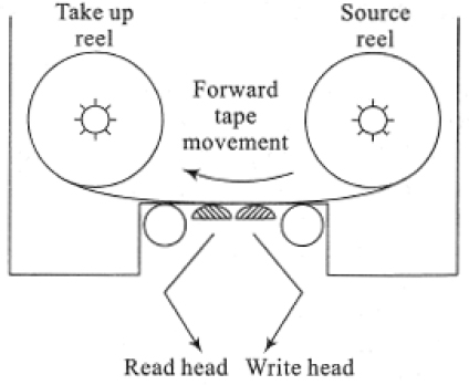
Figure 18.1 Schematic diagram of a magnetic tape drive
The data to be stored on a tape is written onto it in blocks. These blocks may be of fixed or variable size. A gap of ¾” is left between the blocks and is referred to as Inter Block Gap (IBG). The IBG is long enough to permit the tape to accelerate from rest to reach its normal speed before it begins to read the next block. Figure 18.2 shows the IBG of a tape.
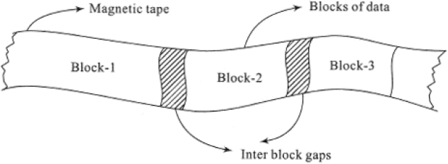
Figure 18.2 Inter block gap of a tape
Magnetic tape is a sequential device since having read a block of data, if one desires to read another block that is several feet down the tape, then it is essential to fast forward the tape until the correct block is reached. Again, if we desire to read blocks of data that occur towards the beginning of the tape, then it is essential that the tape is rewound and the reading starts from the beginning onward. In these aspects, the characteristic of tapes is similar to that of audio cassettes.
18.2.2. Magnetic disks
Magnetic disks are still in vogue and are commonly referred to as hard disks, these days. Hard disks are random access storage devices. This means that hard disks store data in such a manner that they permit both sequential access as well as random or direct access to data.
A disk pack is mountable on a disk drive and comprises platters that are similar to phonograph records. The number of platters in a disk pack varies according to its capacity. Figure 18.3 shows a schematic diagram of a disk pack comprising 6 platters.
Recording of data is done on all surfaces of the platters except the outer surfaces of the first and last platter. Thus, for a 6-platter disk pack, of the 12 surfaces available, data recording is done only on 10 of the surfaces. Each surface is accessed by a read/write head. The access assembly comprises an assembly of access arms ending in the read/write head. The access assembly moves in and out together with the access arms so that all the read/write heads at any point of time are stationed at the same position on the surface. During a read/write operation, the read/write head is held stationary over the appropriate position on the surface, while the disk rotates at high speed to enable the read/write operation. Disk speeds ranging from 3000 rpm to 7200 rpm are common these days.
Each surface of the platter, like a phonograph record, is made up of concentric circles of tracks of decreasing radii, on which the data is recorded. Modern versions of the hard disk contain tens of thousands of tracks per surface. The tracks are numbered from 0 beginning from the outer edge of the platter. The collection of tracks of the same radii, occurring on all the surfaces of the disk pack, is referred to as a cylinder (Figure 18.3). Thus, a disk pack is virtually viewed as a collection of cylinders of decreasing radii. Each track is divided into sectors, which is the smallest addressable segment of a track. Typically, a sector can hold 512 bytes of data approximately. The early disk packs had all tracks holding the same number of sectors. The modern versions have however rid themselves of this feature to increase the storage capacity of the disk.

Figure 18.3 Schematic diagram of a disk pack
To access information on a disk, it is essential to first specify the cylinder number, followed by the track number and the sector number. A multilevel index-based ISAM file organization (section 14.7) is adopted for obtaining the physical locations of records stored on the disk. The cylinder index records the highest key in each cylinder and the cylinder number. The surface index or the track index stores the highest key in each track and the track number. Finally, the sector index records the highest key in each sector and the sector number. In practice, each of the index entries also contains other spatial information to help locate the records efficiently. Thus, the cylinder, track and sector indexes form a hierarchy of indexes that help identify the physical location of the record.
The read/write head moves across the cylinders to position itself on the right cylinder. The time taken to position the read/write head on the correct cylinder is known as seek time. Once the read/write head has positioned itself on the correct track of the cylinder, it has to wait for the right sector in the track to appear under the corresponding read/write head. The time taken for the right sector to appear under the read/write head is known as latency time or rotational delay. Once the sector is reached, the corresponding data is read or written onto the disk. The time taken for the transfer of data to and from the disk is known as data transmission time.
18.3. Sorting with tapes: balanced merge
Balanced merge sort makes use of an internal sorting technique to generate the runs and employs merging to gather the runs for the next phase of the sorting. The repeated run generation and merging continue until a single run generated in the final phase delivers the sorted file.
In this section, we discuss the balanced merge when the file resides on a tape. Besides the input tape, the sorting method has to make use of a few more work tapes to hold the runs that are generated from time to time and to perform the merging of the runs as well. Example 18.1 illustrates a balanced merge sort on tapes. The sorting method makes use of a two-way merge to gather the runs.
18.3.1. Buffer handling
While merging runs in the balanced merge sort procedure, it needs to be observed that due to the limited capacity of the internal memory of the computer, it is not always possible to completely accommodate the runs and the merged list in it. In fact, the problem gets severe as the phases in the sort procedure progress, since the runs get longer and longer.
To tackle this problem, in the case of a two-way merge let us say, we trifurcate the internal memory into blocks known as buffers. Two of these blocks will be used as input buffers and the third as the output buffer. During the merge of two runs R1 and R2, for example, as many records as can be accommodated in the two input buffers are read from the runs R1 and R2 respectively. The merged records are sent to the output buffer. Once the output buffer is full, the records are written onto the disk. If during the merging process, any of the input buffers gets empty, it is once again filled with the rest of the records from the runs.
Example 18.2 presented a naïve view of buffer handling. In reality, issues such as proper choice of buffer lengths, efficient utilization of program buffers to enable maximum overlapping of input/output and CPU processing times need to be attended to.
18.3.2. Balanced P-way merging on tapes
In the case of a balanced two-way merge, if M runs were produced in the internal sorting phase and if 2k−1 < M ≤ 2k then the sort procedure makes ![]() merging passes over the data records.
merging passes over the data records.
Now balanced merging can easily be generalized to the inclusion of T tapes, T ≥ 3. We divide the tapes, T, into two groups, with P tapes on the one side and (T-P) tapes on the other, where 1 ≤ P < T. The initial runs generated after internal sorting are evenly distributed onto the P tapes in the first group. A P-way merge is undertaken and the resulting runs are evenly distributed onto the next group containing (T-P) tapes. This is followed by a (T-P) merge of the runs available on the (T-P) tapes, with the output runs getting evenly distributed onto the P tapes of the first group and so on. However, it has been proved that ![]() is the best choice.
is the best choice.
Illustrative problem 18.4 discusses an example. Though balanced merging can be quite simple in its implementation, it needs to be seen if better merging patterns that save time and resources can be evolved for the specific cases in hand. Illustrative problems 18.5 and 18.6 discuss specific cases.
18.4. Sorting with disks: balanced merge
Tapes being sequential access devices, the balanced merge sort methods had to employ sizable resources for the efficient distribution of runs besides spending time for mounting, dismounting and rewinding tapes. In the case of disks which are random access storage devices, we are spared of this burden. The seek time and latency time to access blocks of data from a disk are comparatively negligible, to the time taken to access blocks of data on tapes.
The balanced merge sort procedure for disk files, though similar in principle to that of tape files, is a lot simpler. The runs generated by the internal sorting methods are repeatedly merged until a single run emerges with the entire file sorted in the final pass. Example 18.3 demonstrates a balanced merge sort on a disk file.
18.4.1. Balanced k-way merging on disks
As discussed in Section 18.3.2, balanced two-way merge sort can be generalized to k-way merging. For a two-way merge, as can be deduced from Figure 18.4, the number of passes over data is given by ![]() where M is the number of runs in the first level of the merge tree. A higher order merge can serve to reduce the number of passes over data. Thus, in the case of a k-way merge, k ≥ 2, the number of passes is given by
where M is the number of runs in the first level of the merge tree. A higher order merge can serve to reduce the number of passes over data. Thus, in the case of a k-way merge, k ≥ 2, the number of passes is given by ![]() , where M is the number of runs. Figure 18.5 shows the merge tree for k = 4, for an initial generation of 16 runs in a specific case.
, where M is the number of runs. Figure 18.5 shows the merge tree for k = 4, for an initial generation of 16 runs in a specific case.

Figure 18.5 Balanced k-way merge sort: merging the runs for k = 4
Though the k-way merge can significantly reduce input/output due to the reduction in the number of passes, it is not without its ill effects. Let us suppose R1, R2, R3, ….Rk are the k runs generated initially with size ri, 1 ≤ i≤ k. During a k-way merge, the next record which is to be output is the one with the smallest key. A direct method to find the smallest key would call for (k-1) comparisons. The computing time to merge the k runs would be given by ![]() . Since
. Since ![]() passes are being made, the total number of key comparisons is given by n(k − 1)log2 M, where n is the total number of records in the source file. We have
passes are being made, the total number of key comparisons is given by n(k − 1)log2 M, where n is the total number of records in the source file. We have ![]() . In other words for a k-way merge sort, the number of key comparisons increases by a factor of
. In other words for a k-way merge sort, the number of key comparisons increases by a factor of ![]() . Thus, for large k (k ≥ 6) the CPU time needed to perform the k-way merge will overweigh the reduction achieved in input/output time due to the reduction in the number of passes. A significant reduction in the number of comparisons to find the smallest key can be achieved by using what is known as a selection tree.
. Thus, for large k (k ≥ 6) the CPU time needed to perform the k-way merge will overweigh the reduction achieved in input/output time due to the reduction in the number of passes. A significant reduction in the number of comparisons to find the smallest key can be achieved by using what is known as a selection tree.
18.4.2. Selection tree
A selection tree is a complete binary tree that serves to obtain the smallest key from among a set of keys. Each internal node represents the smaller of its two children and external nodes represent the keys from which the selection of the smallest key needs to be made. The root node represents the smallest key that was selected.
Figure 18.6(a) represents a selection tree for an eight-way merge. The eight lists to be merged are L1 (5, 7, 8), L2 (6, 9, 9), L3 (2, 4, 5), L4 (1, 7, 8), L5 (3, 6, 9), L6 (5, 5, 6), L7 (3, 4, 9), L8 (6, 8, 9). The external nodes represent the first set of 8 keys that were selected from the lists. Progressing from the bottom up, each of the internal nodes represents the smaller key of its two children until at the root node the smallest key gets automatically represented. The construction of the selection tree can be compared to a tournament being played with each of the internal nodes recording the winners of the individual matches. The final winner is registered by the root node. A selection tree, therefore, is also referred to as a tree of winners.

Figure 18.6 Selection tree for an eight-way merge
In this case, the smallest key, for example, 1 is dropped into the output list. Now the next key from L4 for example, 7 enters the external node. It is now essential to restructure the tree to determine the next winner. Observe how it is now sufficient to restructure only that portion of the tree occurring along the path from the node numbered 11 to the root node. The revised key values of the internal nodes are shown in Figure 18.6(b). Note how in this case, the keys compared and revised along the path are (2,7), (5,2) and (2,3). The root node now represents 2 which is the next smallest key.
In practice, the external nodes of the selection tree are represented by the records and the internal nodes are only pointers to the records which are winners. For ease of understanding the internal nodes in Figure 18.6 were represented using the keys themselves, though in reality, they are only pointers to the winning records.
Despite its merits, a selection tree can result in increased overheads associated with maintaining the tree. This happens especially when the restructuring of the tree takes place to determine the next winner. It can be seen that when the next key walks into the tree, tournaments have to be played between sibling nodes who earlier, were losers.
Note how in the case of 7 entering the tree, the tournaments played were between (2,7), (5,2) and (2,3), where 2, 5 and 3 were losers in the earlier case. It would therefore be prudent if the internal nodes could represent the losers rather than the winners. A tournament tree in which each internal node retains a pointer to the loser is called a tree of losers.
Figure 18.7(a) illustrates the tree of losers for the selection tree discussed in Figure 18.6. Node 0 is a special node that shows the winner. As said earlier, each of the internal nodes is shown carrying the key when in reality they represent only pointers to the loser records. To determine the smallest key, as before, a tournament is played between pairs of external nodes. Though the winners are ‘remembered’, it is the losers that the internal nodes are made to point to. Thus, nodes numbered ((4), (5), (6) and (7)) record pointers to the losing external nodes, which are the ones with the key values of 6, 2, 5 and 6, respectively. Now node numbered (2) conducts a tournament between the two winners of the earlier game, which are key values 5 and 1 and records the pointer to the loser which is 5. In a similar way, node numbered (3) records the pointer to the loser node with key value 3. Progressing in this way the tree of losers is constructed and node 0 outputs the winning key value which is the smallest.
Once the smallest key, which is 1 has been output and the next key 7 enters the tree, the restructuring is easier now since the sibling nodes with which the tournaments are to be played are losers and these are directly pointed to by the internal nodes. The restructured tree is shown in Figure 18.7(b).
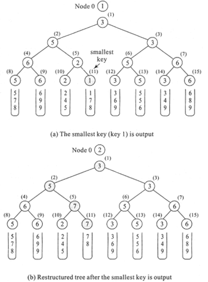
Figure 18.7 Tree of losers for the eight-way merge
18.5. Polyphase merge sort
Balanced k-way merge sort on tapes calls for an even distribution of runs on the tapes and to enable efficient merging requires 2k tapes to avoid wasteful passes over data. Thus, while k tapes act as input devices holding the runs generated, the other k tapes act as output devices to receive the merged runs. The k tape groups swap roles in the successive passes until a single run emerges in one of the tapes, signaling the end of sort.
It is possible to avoid wasteful redistribution of runs on the tapes while using less than 2k tapes by a wisely thought-out run redistribution strategy. Polyphase merge is one such external sorting method that makes use of an intelligent redistribution of runs during merging, so much that a k-way merge requires only (k+1) tapes!
The central principle of the method is to ensure that in each pass (except the last of course!) during the merge, the runs are to be cleverly distributed so that one tape is always rendered empty while the other k tapes hold the input runs that are to be merged! The empty tape for the current pass acts as the output tape for the next pass and so on. Ultimately, as in balanced merge sort, the final pass delivers only one run in one of the tapes.
At this point of time, we introduce a useful notation mentioned in the literature to enable a crisp presentation of run distribution. Runs that are initially generated by internal sorting are thought to be of length 1 (unit of measure). Thus, if there are t runs that are initially generated then the notation would describe it as 1t. For example, if there were 34 runs that were initially generated then it would be represented as 134. Similarly, if after a merge there were 14 runs of size 2, it would be represented as 214. In general, t runs of size s would be represented as st.
Example 18.4 illustrates polyphase merge on 3 tapes.
Let us suppose that ‘intuitively’ we decided to distribute 13 runs of size 1 and 21 runs of size 1 onto tapes T1 and T2 respectively. In phase 2, because it is a two-way merge and polyphase merge expects one tape to fall vacant in every phase, we use up all the 13 runs of size 1 in tape T1 for a merge operation with an equivalent number of runs in tape T2. This yields 13 runs of double the size (213) which is written onto the empty tape T3. So that leaves 8 runs of size 1 on tape T2 that could not be used up and renders tape T1 empty. Again, in phase 3, 18 runs in tape T2 are merged with an equivalent amount of runs in tape T3 to obtain 38 which is written onto tape T1. This leaves a balance of 25 runs on tape T3 and renders tape T2 empty. The phases continue until in phase 8 a single run 341 gets written onto tape T3.
To determine how the initial distribution of 113 and 121 was conceived, we work backward from the last phase. Let us suppose there were n phases for a 3-tape case. In the nth phase, we should arrive at exactly one run on a tape T1 (let us say) with tapes T2 and T3 totally empty. This implies that in phase (n-1) there should have been two runs of size 1 on tapes T2 and T3, which should have been merged as a single run on T3 in the nth phase. Continuing in this fashion we obtain the initial distribution of runs to be 113 and 121 on the two tapes respectively. Table 18.2 lists the run distribution for a 3-tape polyphase merge.
It can be easily seen that the number of runs needed for an n-phase merge is given by Fn + Fn-1 where Fi is the ith Fibonacci number. Hence, this method of redistribution of runs is known as the Fibonacci merge. The method can be clearly generalized to k-way merging on (k+1) tapes using generalized Fibonacci numbers.
Table 18.2 Run distribution for a 3-tape polyphase merge
| Phase | Tape T1 | Tape T2 | Tape T3 |
|---|---|---|---|
| n | 0 | 0 | 1 |
| n-1 | 1 | 1 | 0 |
| n-2 | 2 | 0 | 1 |
| n-3 | 0 | 2 | 3 |
| n-4 | 3 | 5 | 0 |
| n-5 | 8 | 0 | 5 |
| n-6 | 0 | 8 | 13 |
| n-7 | 13 | 21 | 0 |
| n-8 | 34 | 0 | 21 |
18.6. Cascade merge sort
Cascade merge is another intelligent merge pattern that was discovered before the polyphase merge. The merge pattern makes use of a perfectly devised initial distribution of runs on the tapes. While the polyphase merge sort employs a uniform merge pattern during the run generation, the cascade merge sort makes use of a ‘cascading’ merge pattern in each of its passes. Thus, for t tapes, while polyphase merge uniformly employs a (t-1) merge for the run generation, cascade sort employs (t-1) merge, (t-2) merge and so on, in the same pass for its run generation.
Example 18.5 demonstrates cascade merge on 6 tapes for an initial generation of 55 runs of length 1. We make use of the run distribution notation introduced in section 18.5.
As before, let us assume that the initial distribution of (115, 114, 112, 19, 15) runs on the tapes (T1, T2, T3, T4, T5), was devised through some ‘intuitive’ means.
In pass 1, we undertake a series of merges. A five-way merge on (T1, T2, T3, T4, T5) yields the run 55 that is put onto tape T6. A four-way merge on (T1, T2, T3, T4) yields 44 which is put onto tape T5. A three-way merge on (T1, T2, T3) yields 33 which are distributed onto tape T4. A two-way merge on (T1, T2) yields 22 which is put onto tape T3. Lastly, a 1-way merge (which is mere copying of the balance run) on T1 yields 11 which is copied onto tape T2. Of course, one could do away with the 1-way merge which is mere copying of the run and retain the run in the very tape itself. In pass 1, tape T1 falls empty.
In pass 2, we repeat the cascading merge wherein the five-way merge on (T2, T3, T4, T5, T6) yields the run 151, a four-way merge on (T3, T4, T5, T6) yields 141 and so on until at the end of pass 2, the distribution of runs on the tapes is as shown in the table. This is the penultimate pass and observes how the distribution records one run each on the tapes. In the final pass, as it always is, the five-way merge releases a single run of size 55 which is the final sorted file.
Table 18.4 Run distribution on five tapes by cascade merge
| Phase | T1 | T2 | T3 | T4 | T5 |
|---|---|---|---|---|---|
| n | 1 | 0 | 0 | 0 | 0 |
| n-1 | 1 | 1 | 1 | 1 | 1 |
| n-2 | 5 | 4 | 3 | 2 | 1 |
| n-3 | 15 | 14 | 12 | 9 | 5 |
| n-4 | 55 | 50 | 41 | 29 | 15 |
| n-5 | 190 | 175 | 146 | 105 | 55 |
| n-6 | 671 | 616 | 511 | 365 | 190 |
Now, how does one arrive at the perfect initial distribution? As was done for polyphase merge, this could be arrived at by working backward from the goal state of (1, 0, 0, 0, 0) obtained during the nth pass. Table 18.4 illustrates the run distribution by cascade merge on five tapes.
For an in-depth analysis of merge patterns and other external sorting schemes, a motivated reader is referred to Volume III of the classic book “The ART of Computer Programming” (Knuth 1998).
Summary
- External sorting deals with sorting of files or lists that are too huge to be accommodated in the internal memory of the computer and hence need to be stored in external storage devices such as disks or drums.
- The principle behind external sorting is to first make use of any efficient internal sorting technique to generate runs. These runs are then merged in passes to obtain a single run at which stage the file is deemed sorted. The merge patterns called for by the strategies, are influenced by external storage medium on which the runs reside, viz., disks or tapes.
- Magnetic tapes are sequential devices built on the principle of audio tape devices. Data is stored in blocks occurring sequentially. Magnetic disks are random access storage devices. Data stored in a disk is addressed by its cylinder, track and sector numbers.
- Balanced merge sort is a technique that can be adopted on files residing on both disks and tapes. In its general form, a k-way merging could be undertaken during the runs. For the efficient management of merging runs, buffer handling and selection tree mechanisms are employed.
- Balanced k-way merge sort on tapes calls for the use of 2k tapes for an efficient management of runs. Polyphase merge sort is a clever strategy that makes use of only (k+1) tapes to perform the k –way merge. The distribution of runs on the tapes follows a Fibonacci number sequence.
- Cascade merge sort is yet another smart strategy which unlike polyphase merge sort does not employ a uniform merge pattern. Each pass makes use of a ‘cascading’ sequence of merge patterns.
18.7. Illustrative problems
Review questions
- Cascade merge sort adopts uniform merge patterns in its passes.
- The distribution of runs in the last pass of cascade merge sort is given by a pattern such as (1, 0, 0, …0).
- true
- true
- true
- false
- false
- false
- false
- true
- Polyphase merge sort for a k-way merge on tapes requires ------------ tapes.
- 2k
- (k-2)
- (k+1)
- k
- The time taken for the right sector to appear under the read/write head is known as:
- seek time
- latency time
- transmission time
- data read time
- In the case of a balanced two-way merge, if M runs were produced in the internal sorting phase and if then the sort procedure makes --------- merging passes over the data records.
- M


- M2
- Match the following:
W. Magnetic tape A. tree of winners X. Magnetic disks B. Fibonacci merge Y. Polyphase merge C. Inter Block Gap Z. k-way merge D. platters - (W A) (X B) (Y D) (Z C)
- (W C) (X D) (Y B) (Z A)
- (W C) (X D) (Y A) (Z B)
- (W A) (X B) (Y C) (Z D)
- What is the general principle behind external sorting?
- How is a selection tree useful in a k-way merge?
- What are the advantages of Polyphase merge sort over balanced k-way merge sort?
- What is the principle behind the distribution of runs in a cascade merge sort?
- How is data organized in a magnetic disk?
- An inventory record contains the following fields: ITEM NUMBER (8 bytes), NAME (20 bytes), DESCRIPTION (20 bytes), TOTAL STOCK (10 bytes), PRICE(10 bytes), TOTAL PRICE (14 bytes).
A record comprising the data on Item number, name, description and total stock is to be read and based on the current price which is input, the total price is to be computed and updated in the fields. There are 25, 000 records to be processed. Assuming the disk characteristics given in Table P18.1:
- How much storage space is required to store the entire file in the disk (in terms of bytes/KB/MB)?
- How much storage space is required to store the entire file in the disk in terms of cylinders?
- What is the time required to read, process and write back a given sector of records into the disk, assuming that it takes 100 µs to process a record?
- What is the time required to read, process and write back an entire track of records if they were read sequentially sector after sector?
- What is the time required to read, process and write back an entire cylinder of records?
- What is the time required to read, process and write back the records in the next (immediate) cylinder?
- What is the time required to read, process and write back the entire file onto the disk?
- A file comprising 500,000 records is to be sorted. The internal memory has the capacity to hold only 50,000 records. Trace the steps of a Balanced k-way merge for (i) k = 2 and (ii) k = 4, when (a) the file is available on a tape and (ii) the file is available on a disk. Assume the availability of any number of tapes and a scratch disk for undertaking the appropriate sorting process.
Programming assignments
- Implement a function to construct a tree of winners to obtain the smallest key from a list of keys representing its external nodes.
- Implement a function to construct a tree of losers to obtain the smallest key from a list of keys representing its external nodes.
- Making use of the function(s) developed in programming assignment 1 (and programming assignment 2), implement k-way merge algorithms for any given value of k.
- Implement a balanced k-way merge sort for disk-based files. Simulate the program for various sizes of files, internal memory capacity and choice of k. Graphically display the distribution of runs.