
17
Internal Sorting
17.1. Introduction
Sorting in the English language refers to separating or arranging things according to different classes. However, in computer science, sorting, also referred to as ordering, deals with arranging elements of a list or a set or records of a file in ascending or descending order.
In the case of sorting a list of alphabetical, numerical or alphanumerical elements, the elements are arranged in ascending or descending order based on their alphabetical or numerical sequence number. The sequence is also referred to as a collating sequence. In the case of sorting a file of records, one or more fields of the records are chosen as the key based on which the records are arranged in ascending or descending order.
Examples of lists before and after sorting are shown below:
| Unsorted lists | Sorted lists |
|---|---|
| {34, 12, 78, 65, 90, 11, 45} | {11, 12, 34, 45, 65, 78, 90} |
| {tea, coffee, cocoa, milk, malt, chocolate} | {chocolate, cocoa, coffee, malt, milk, tea} |
| {n12x, m34b, n24x, a78h, g56v, m12k, k34d} | {a78h, g56v, k34d, m12k, m34b, n12x, n24x} |
Sorting has acquired immense significance in the discipline of computer science. Several data structures and algorithms display efficient performance when presented with sorted data sets.
Many different sorting algorithms have been invented, each having their own advantages and disadvantages. These algorithms may be classified into families such as sorting by exchange, sorting by insertion, sorting by distribution, sorting by selection and so on. However, in many cases, it is difficult to classify the algorithms as belonging to a specific family only.
A sorting technique is said to be stable if keys that are equal retain their relative orders of occurrence, even after sorting. In other words, if K1 and K2 are two keys such that K1 = K2, and p(K1) < p(K2 ) where p(Ki) is the position index of the keys in the unsorted list, then after sorting, p’(K1 ) < p’(K2 ), where p’(Ki) is the position index of the keys in the sorted list.
If the list of data or records to be sorted are small enough to be accommodated in the internal memory of the computer, then it is referred to as internal sorting. On the other hand, if the data list or records to be sorted are voluminous and are accommodated in external storage devices such as tapes, disks and drums, then the sorting undertaken is referred to as external sorting. External sorting methods are quite different from internal sorting methods and are discussed in Chapter 18.
In this chapter, we discuss the internal sorting techniques of bubble sort, insertion sort, selection sort, merge sort, shell sort, quick sort, heap sort, radix sort, counting sort and bucket sort.
17.2. Bubble sort
Bubble sort belongs to the family of sorting by exchange or transposition, where during the sorting process, pairs of elements that are out of order are interchanged until the whole list is ordered. Given an unordered list L = {K1, K2, K3, … Kn} bubble sort orders the elements in ascending order (i.e.), L = {K1, K2, K3, … Kn}, K1 ≤ K2 ≤ … Kn.
Given the unordered list L = {K1, K2, K3, … Kn} of keys, bubble sort compares pairs of elements Ki and Kj, swapping them if Ki > Kj. At the end of the first pass of comparisons, the largest element in the list L moves to the last position in the list. In the next pass, the sublist {K1, K2, K3, … Kn − 1} is considered for sorting. Once again the pair-wise comparison of elements in the sublist results in the next largest element floating to the last position of the sublist. Thus, in (n-1) passes, where n is the number of elements in the list, the list L is sorted. The sorting is called bubble sorting for the reason that with each pass the next largest element of the list floats or “bubbles” to its appropriate position in the sorted list.
Algorithm 17.1 illustrates the procedure for bubble sort.
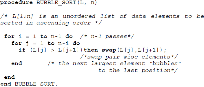
Algorithm 17.1 Procedure for bubble sort
In the second pass, the list considered for sorting discounts the last element, which is 92, since 92 has found its rightful position in the sorted list. At the end of the second pass, the next largest element, which is 90, would have moved to the end of the list. The partially sorted list at this point would be {34, 23, 56, 78, 17, 52, 67, 81, 18, 90, 92}. The elements shown in boldface and underlined, indicate elements discounted from the sorting process.
In pass 10 the whole list would be completely sorted.
The trace of algorithm BUBBLE_SORT (Algorithm 17.1) over L is shown in Table 17.1. Here, i keeps count of the passes and j keeps track of the pair-wise element comparisons within a pass. The lower (l) and upper (u) bounds of the loop controlled by j in each pass are shown as l..u. Elements shown in boldface and underlined in the list L at the end of pass i, indicate those discounted from the sorting process.

Table 17.1 Trace of Algorithm 17.1 over the list L = {92, 78, 34, 23, 56, 90, 17, 52, 67, 81, 18}
17.2.1. Stability and performance analysis
Bubble sort is a stable sort since equal keys do not undergo swapping, as can be observed in Algorithm 17.1, and this contributes to the keys maintaining their relative orders of occurrence in the sorted list.
17.3. Insertion sort
Insertion sort as the name indicates belongs to the family of sorting by insertion, which is based on the principle that a new key K is inserted at its appropriate position in an already sorted sub-list.
Given an unordered list L = {K1, K2, K3, … Kn}, insertion sort employs the principle of constructing the list L = {K1, K2, K3, … Ki, K, Kj, Kj+1, … .Kn}, K1 ≤ K2 ≤ … Ki and inserting a key K at its appropriate position by comparing it with its sorted sublist of predecessors {K1, K2, K3, … Ki}, K1 ≤ K2 ≤ … Ki for every key K (K = Ki, i = 2,3,..n) belonging to the unordered list L.
In the first pass of insertion sort, K2 is compared with its sorted sublist of predecessors, which is K1. K2 inserts itself at the appropriate position to obtain the sorted sublist {K1, K2}. In the second pass, K3 compares itself with its sorted sublist of predecessors which is {K1, K2}, to insert itself at its appropriate position, yielding the sorted list {K1, K2, K3} and so on. In the (n-1)th pass, Kn compares itself with its sorted sublist of predecessors {K1, K2, ….Kn-1}, and having inserted itself at the appropriate position, yields the final sorted list L = {K1, K2, K3, … Ki, … Kj, … Kn}, K1 ≤ K2 ≤ … Ki ≤ … ≤ Kj ≤ … Kn. Since each key K finds its appropriate position in the sorted list, such a technique is referred to as the sinking or sifting technique.
Algorithm 17.2 illustrates the procedure for insertion sort. The for loop in the algorithm keeps count of the passes and the while loop implements the comparison of the key key with its sorted sublist of predecessors. As long as the preceding element in the sorted sublist is greater than key, the swapping of the element pair is done. If the preceding element in the sorted sublist is less than or equal to key, then key is left at its current position and the current pass terminates.
17.3.1. Stability and performance analysis

Algorithm 17.2 Procedure for insertion sort
Insertion sort is a stable sort. It is evident from the algorithm that the insertion of key K at its appropriate position in the sorted sublist affects the position index of the elements in the sublist as long as the elements in the sorted sublist are greater than K. When the elements are less than or equal to the key K, there is no displacement of elements and this contributes to retaining the original order of keys which are equal in the sorted sublists.
The stability of insertion sort can be easily verified in this example. Observe how keys that are equal maintain their original relative orders of occurrence in the sorted list.
The worst-case performance of insertion sort occurs when the elements in the list are already sorted in descending order. It is easy to see that in such a case every key that is to be inserted has to move to the front of the list and therefore undertakes the maximum number of comparisons. Thus, if the list L = {K1, K2, K3, … Kn}, K1 ≥ K2 ≥ … Kn is to be insertion sorted then the number of comparisons for the insertion of key Ki would be (i-1), since Ki would swap positions with each of the (i-1) keys occurring before it until it moves to position 1. Therefore, the total number of comparisons for inserting each of the keys is given by

The best case complexity of insertion sort arises when the list is already sorted in ascending order. In such a case, the complexity in terms of comparisons is given by O(n). The average case performance of insertion sort reports O(n2) complexity.
17.4. Selection sort
Selection sort is built on the principle of repeated selection of elements satisfying a specific criterion to aid the sorting process.
The steps involved in the sorting process are listed below:
- Given an unordered list L = {K1, K2, K3, … Kj … Kn}, select the minimum key K.
- Swap K with the element in the first position of the list L, which is K1. By doing so the minimum element of the list has secured its rightful position of number one in the sorted list. This step is termed pass 1.
- Exclude the first element and select the minimum element K from amongst the remaining elements of the list L. Swap K with the element in the second position of the list, which is K2. This is termed pass 2.
- Exclude the first two elements which have occupied their rightful positions in the sorted list L. Repeat the process of selecting the next minimum element and swapping it with the appropriate element, until the entire list L gets sorted in the ascending order. The entire sorting gets done in (n-1) passes.
Selection sort can also sort in descending order by selecting the maximum element instead of the minimum element and swapping it with the element in the last position of the list L.
Algorithm 17.3 illustrates the working of selection sort. The procedure FIND_MINIMUM (L,i,n) selects the minimum element from the array L[i:n] and returns the position index of the minimum element to procedure SELECTION_SORT. The for loop in the SELECTION_SORT procedure represents the (n-1) passes needed to sort the array L[1:n] in the ascending order. Function swap swaps the elements input into it.

Algorithm 17.3 Procedure for selection sort
17.4.1. Stability and performance analysis
Selection sort is not stable. Example 17.6 illustrates a case.
The computationally expensive portion of the selection sort occurs when the minimum element has to be selected in each pass. The time complexity of the FIND_MINIMUM procedure is O(n). The time complexity of the SELECTION_SORT procedure is, therefore, O(n2).
17.5. Merge sort
Merging or collating is a process by which two ordered lists of elements are combined or merged into a single ordered list. Merge sort makes use of the principle of the merge to sort an unordered list of elements and hence the name. In fact, a variety of sorting algorithms belonging to the family of sorting by merge exist. Some of the well-known external sorting algorithms belong to this class.
17.5.1. Two-way merging
Two-way merging deals with the merging of two ordered lists.
Let L1 = {a1, a2, … ai … an} a1 ≤ a2 ≤ … ≤ ai ≤… an and
L2 = {b1, b2,…bj,…bm} b1 ≤ b2 ≤ … ≤ bj ≤ … bm be two ordered lists. Merging combines the two lists into a single list L by making use of the following cases of comparison between the keys ai and bj belonging to L1 and L2, respectively:
A1. If ( ai < bj ) then drop ai into the list L
A2. If ( ai > bj ) then drop bj into the list L
A3. If ( ai = bj ) then drop both ai and bj into the list L
In the case of A1, once ai is dropped into the list L, the next comparison of bj proceeds with ai+1. In the case of A2, once bj is dropped into the list L, the next comparison of ai proceeds with bj+1. In the case of A3, the next comparison proceeds with ai+1 and bj+1. At the end of merge, list L contains (n+m) ordered elements.
The series of comparisons between pairs of elements from the lists L1 and L2 and the dropping of the relatively smaller elements into the list L proceeds until one of the following cases happens:
B1. L1 gets exhausted earlier to that of L2. In such a case, the remaining elements in list L2 are dropped into the list L in the order of their occurrence in L2 and the merge is done.
B2. L2 gets exhausted earlier to that of L1. In such a case the remaining elements in list L1 are dropped into the list L in the order of their occurrence in L1 and the merge is done.
B3. Both L1 and L2 are exhausted, in which case the merge is done.

Figure 17.1 Two-way merge
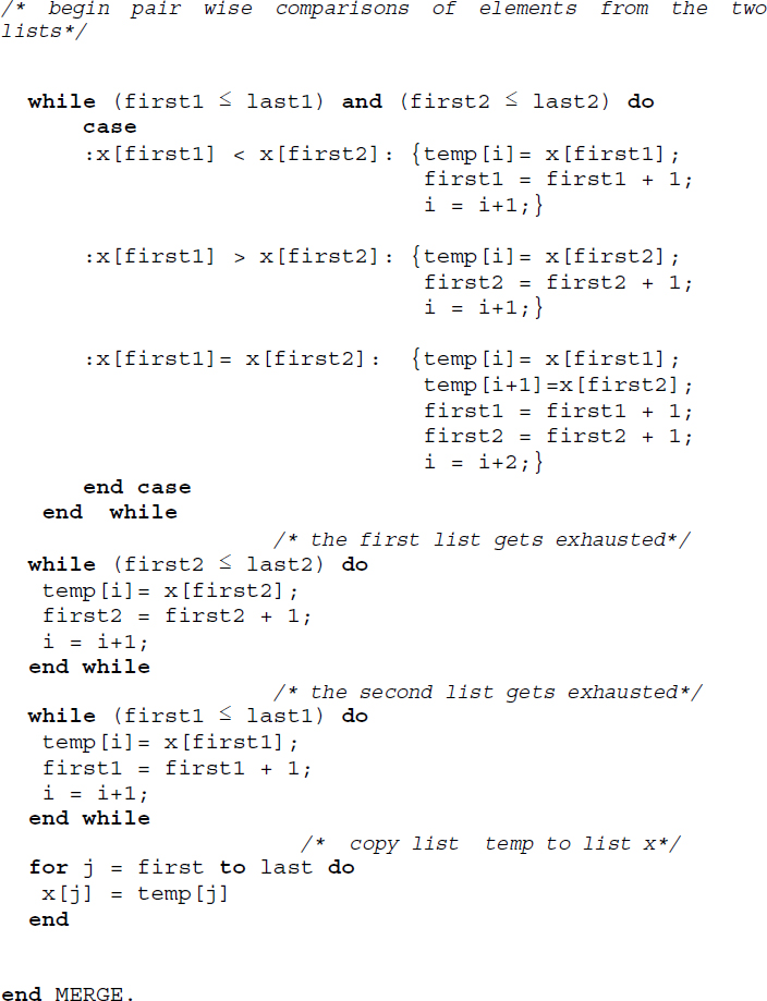
Algorithm 17.4 illustrates the procedure for merge. Here, the two ordered lists to be merged are given as (x1, x2, … xt) and (xt+1, xt+2,… xn) to enable reuse of the algorithm for merge sort to be discussed in the subsequent section. The input parameters to procedure MERGE are given as (x, first, mid, last), where first is the starting index of the first list, mid is the index related to the end/beginning of the first and second list respectively and last is the ending index of the second list.
The call to merge the two lists, (x1, x2, … xt) and (xt+1, xt+2,… xn) would be MERGE(x, 1, t, n). While the first while loop in the procedure performs the pair-wise comparison of elements in the two lists, as discussed in cases A1–A3, the second while loop takes care of case B1 and the third loop take care of case B2. Case B3 is inherently taken care of in the first while loop.
17.5.1.1. Performance analysis
The first while loop in Algorithm 17.4 executes at most (last-first+1) times and plays a significant role in the time complexity of the algorithm. The rest of the while loops only move the elements of the unexhausted lists into the list x. The complexity of the first while loop and hence the algorithm is given by O(last-first+1).
In the case of merging two lists (x1, x2, … xt), (xt+1, xt+2,… xn) where the number of elements in the two lists sums to n, the time complexity of MERGE is given by O(n).
17.5.2. k-way merging
The two-way merge principle could be extended to k-ordered lists in which case it is termed k-way merging. Here, k ordered lists

each comprising n1, n2, …nk number of elements are merged into a single ordered list L comprising (n1+ n2+ …nk ) number of elements. At every stage of comparison, k keys aij, one from each list, are compared before the smallest of the keys are dropped into the list L. Cases A1–A3 and B1–B3, discussed in section 17.5.1 with regard to two-way merge, also hold true in this case, but are extended to k lists. Illustrative problem 17.3 discusses an example k-way merge.
17.5.3. Non-recursive merge sort procedure
Given a list L = {K1, K2, K3, … Kn} of unordered elements, merge sort sorts the list making use of procedure MERGE repeatedly over several passes.
The non-recursive version of merge sort merely treats the list L of n elements as n independent ordered lists of one element each. In pass one, the n singleton lists are pair-wise merged. At the end of pass 1, the merged lists would have a size of 2 elements each. In pass 2, the lists of size 2 are pair-wise merged to obtain ordered lists of size 4 and so on. In the ith pass, the lists of size 2(i-1) are merged to obtain ordered lists of size 2(i).
During the passes, if any of the lists are unable to find a pair for their respective merge operation, then they are simply carried forward to the next pass.
17.5.3.1. Performance analysis
Merge sort proceeds by running several passes over the list that is to be sorted. In pass 1 sublists of size 1 are merged, in pass 2 sublists of size 2 are merged and in the ith pass sublists of size 2(i-1) are merged. Thus, one could expect a total of ![]() passes over the list. With the merge operation commanding O(n) time complexity, each pass of merge sort takes O(n) time. The time complexity of merge sort, therefore, turns out to be O(n.log2 n).
passes over the list. With the merge operation commanding O(n) time complexity, each pass of merge sort takes O(n) time. The time complexity of merge sort, therefore, turns out to be O(n.log2 n).
17.5.3.2. Stability
Merge sort is a stable sort since the original relative orders of occurrence of repeating keys are maintained in the sorted list. Illustrative problem 17.4 demonstrates the stability of the sort over a list.
17.5.4. Recursive merge sort procedure
The recursive merge sort procedure is built on the design principle of Divide and Conquer. Here, the original unordered list of elements is recursively divided roughly into two sublists until the sublists are small enough where a merge operation is done before they are combined to yield the final sorted list.
Algorithm 17.5 illustrates the recursive merge sort procedure. The procedure makes use of MERGE (Algorithm 17.4) for its merging operation.
17.5.4.1. Performance analysis
Recursive merge sort follows a Divide and Conquer principle of algorithm design. Let T(n) be the time complexity of MERGE_SORT where n is the size of the list. The recurrence relation for the time complexity of the algorithm is given by

Here ![]() is the time complexity for each of the two recursive calls to
is the time complexity for each of the two recursive calls to MERGE_SORT over a list of size n/2 and d is a constant. O(n) is the time complexity of merge. Framing the recurrence relation as
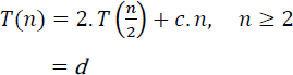
where c is a constant and solving the relation yields the time complexity T(n) = O(n.log2 n) (see illustrative problem 17.5).
17.6. Shell sort
Insertion sort (section 17.3) moves items only one position at a time and therefore reports a time complexity of O(n2) on average. Shell sort is a substantial improvement over insertion sort in the sense that elements move in long strides rather than single steps, thereby yielding a comparatively short subfile or a comparatively well-ordered subfile that quickens the sorting process.
The shell sort procedure was proposed by Shell (1959). The general idea behind the method is to choose an increment ht and divide a list of unordered keys L = {K1, K2, K3, … Kj … Kn} into sub-lists of keys that are ht units apart. Each of the sub-lists is individually sorted (preferably insertion sorted) and gathered to form a list. This is known as a pass. Now we repeat the pass for any sequence of increments {ht−1, ht−2, .… h2, h1, h0} where h0 must equal 1. The increments ht are kept in the diminishing order and therefore shell sort is also referred to as diminishing increment sort.

Algorithm 17.4 Procedure for merge
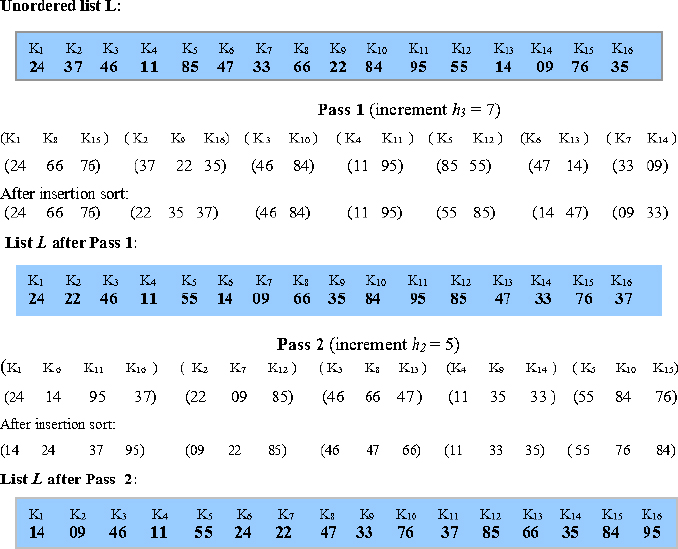
Example 17.10 illustrates shell sort on the given list L for an increment sequence {8, 4, 2, 1}.
In Pass 2, for increment 4, the list gets divided into four groups, each comprising elements which are four units apart in the list L. The individual sub-lists are again insertion sorted and gathered together for the next pass and so on until in Pass 4 the entire list gets sorted for an increment 1.
The shell sort, in fact, could work for any sequence of increments as long as h0 equals 1. Several empirical results and theoretical investigations have been undertaken regarding the conditions to be followed by the sequence of increments. Example 17.11 illustrates shell sort for the same list L used in Example 17.10, but for a different sequence of increments, for example, {7, 5, 3, 1}.
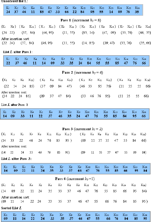
Figure 17.4 Shell sorting of L = {24, 37, 46, 11, 85, 47, 33, 66, 22, 84, 95, 55, 14, 09, 76, 35} for the increment sequence {8, 4, 2, 1}
Figure 17.5 illustrates the steps involved in the sorting process. In Pass 1, the increment of 7 divides the sublist L into seven groups of a varying number of elements. The sub-lists are insertion sorted and gathered for the next pass. In Pass 2, for an increment of 5, the list L gets divided into five groups of a varying number of elements. As before, they are insertion sorted and so on until in Pass 4 the entire list gets sorted for an increment of 1.
Algorithm 17.6 describes the skeletal shell sort procedure. The array L[1:n] represents the unordered list of keys, L = {K1, K2, K3, … Kj … Kn}. H is the sequence of increments {ht, ht−1, ht−2, … h2, h1, h0}.
xs
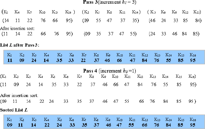
Figure 17.5 Shell sorting of L = {24, 37, 46, 11, 85, 47, 33, 66, 22, 84, 95, 55, 14, 09, 76, 35} for the increment sequence {7, 5, 3, 1}
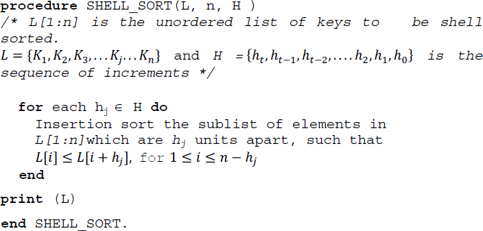
Algorithm 17.6 Procedure for shell sort
17.6.1. Analysis of shell sort
The analysis of shell sort is dependent on a given choice of increments. Since there is no best possible sequence of increments that have been formulated, especially for large values of n (the size of the list L), the time complexity of shell sort is not completely resolved. In fact, it has led to some interesting mathematical problems! An interested reader is referred to Knuth (2002) for discussions on these results.
17.7. Quick sort
The quick sort procedure formulated by Hoare (1962) belongs to the family of sorting by exchange or transposition, where elements that are out of order are exchanged amongst themselves to obtain the sorted list.
The procedure works on the principle of partitioning the unordered list into two sublists at every stage of the sorting process based on what is called a pivot element. The two sublists occur to the left and right of the pivot element. The pivot element determines its appropriate position in the sorted list and is therefore freed of its participation in the subsequent stages of the sorting process. Again, each of the sublists is partitioned against their respective pivot elements until no more partitioning can be called for. At this stage, all the elements would have determined their appropriate positions in the sorted list and a quick sort is done.
17.7.1. Partitioning
Consider an unordered list L = {K1, K2, K3,…Kn}. How does partitioning occur? Let us choose K1 to be the pivot element. Now, K1 compares itself with each of the keys on a left to right encounter looking for the first key Ki, Ki ≥ K. Again, K compares itself with each of the keys on a right to left encounter looking for the first key Kj, Kj ≤ K. If Ki and Kj are such that i < j, then Ki and Kj are exchanged. Figure 17.6(a) illustrates the process of exchange.
Now, K moves ahead from position index i on a left to right encounter looking for a key Ks, Ks ≥ K. Again, as before, K moves on a right to left encounter beginning from position index j looking for a key Kt, Kt ≤ K. As before, if s < t, then Ks and Kt are exchanged and the process repeats (Figure 17.6(b)). If s > t, then K exchanges itself with Kt, the key which is the smaller of Ks and Kt. At this stage, a partition is said to occur. The pivot element K, which has now exchanged position with Kt, is the median around which the list partitions itself or splits itself into two. Figure 17.6(c) illustrates partition. Now, what do we observe about the partitioned sublists and the pivot element?
- The sublist occurring to the left of the pivot element K (now at position t) has all its elements less than or equal to K and the sublist occurring to the right of the pivot element K has all its elements greater than or equal to K.
- The pivot element has settled down in its appropriate position which would turn out to be its rank in the sorted list.
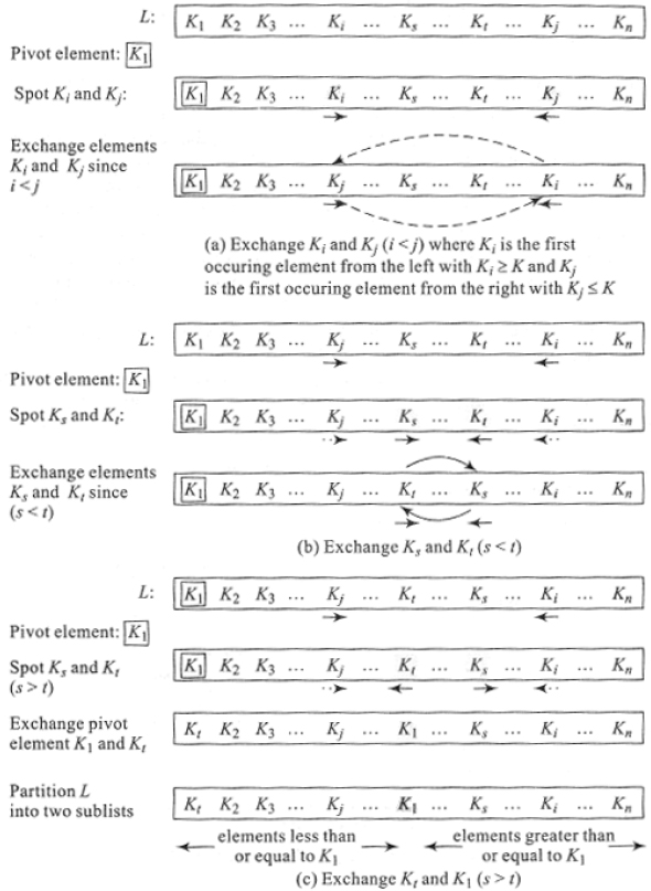
Figure 17.6 Partitioning in quick sort
17.7.2. Quick sort procedure
Once the method behind partitioning is known, quick sort is nothing but repeated partitioning until every pivot element settles down to its appropriate position, thereby sorting the list.
Algorithm 17.8 illustrates the quick sort procedure. The algorithm employs the Divide and Conquer principle by exploiting procedure PARTITION (Algorithm 17.7) to partition the list into two sublists and recursively call procedure QUICK_SORT to sort the two sublists.
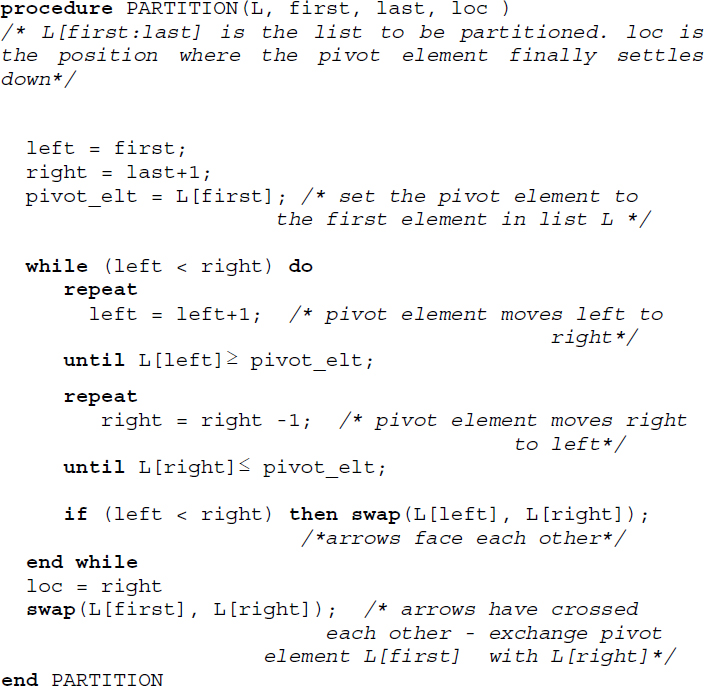
Algorithm 17.7 Procedure for partition
Procedure PARTITION partitions the list L[first:last] at the position loc where the pivot element settles down.
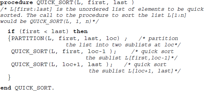
Algorithm 17.8 Procedure for quick sort
17.7.3. Stability and performance analysis
Quick sort is not a stable sort. During the partitioning process, keys which are equal are subject to exchange and hence undergo changes in their relative orders of occurrence in the sorted list.
Quick sort reports a worst-case performance when the list is already sorted in its ascending order (see illustrative problem 17.6). The worst-case time complexity of the algorithm is given by O(n2). However, quick sort reports a good average case complexity of O(n logn).
17.8. Heap sort
Heap sort is a sorting procedure belonging to the family of sorting by selection. This class of sorting algorithms is based on the principle of repeated selection of either the smallest or the largest key from the remaining elements of the unordered list and their inclusion in an output list. At every pass of the sort, the smallest or the largest key is selected by a well-devised method and added to the output list, and when all the elements have been selected, the output list yields the sorted list.
Heap sort is built on a data structure called heap and hence the name heap sort. The heap data structure aids the selection of the largest (or smallest) key from the remaining elements of the list. Heap sort proceeds in two phases as follows:
- construction of a heap where the unordered list of elements to be sorted are converted into a heap;
- repeated selection and inclusion of the root node key of the heap into the output list after reconstructing the remaining tree into a heap.
17.8.1. Heap
A heap is a complete binary tree in which each parent node u labeled by a key or element e(u) and its respective child nodes v, w labeled e(v), e(w) respectively are such that e(u) ≥ e(v) and e(u) ≥ e(w). Since the parent node keys are greater than or equal to their respective child node keys at each level, the key at the root node would turn out to be the largest amongst all the keys represented as a heap.
It is also possible to define the heap such that the root holds the smallest key for which every parent node key should be less than or equal to that of its child nodes. However, by convention, a heap sticks to the principle of the root holding the largest element. In the case of the former, it is referred to as a minheap and in the case of the latter, it is known as a maxheap. A binary tree that displays this property is also referred to as a binary heap.
It may be observed in Figure 17.10(a) how each parent node key is greater than or equal to that of its child node keys. As a result, the root represents the largest key in the heap. In contrast, the non-heap shown in Figure 17.10(b) violates the above characteristics.
17.8.2. Construction of heap
Given an unordered list of elements, it is essential that a heap is first constructed before heap sort works on it to yield the sorted list. Let L = {K1, K2, K3,…Kn} be the unordered list. The construction of the heap proceeds by inserting keys from L one by one into an existing heap. K1 is inserted into the initially empty heap as its root. K2 is inserted as the left child of K1. If the property of heap is violated then K1 and K2 swap positions to construct a heap out of themselves. Next K3 is inserted as the right child of node K1. If K3 violates the property of heap, it swaps position with its parent K1 and so on.
In general, a key Ki is inserted into the heap as the child of node ![]() following the principle of a complete binary tree (the parent of child i is given by
following the principle of a complete binary tree (the parent of child i is given by ![]() and the right and left child of i is given by 2i and (2i+1) respectively). If the property of the heap is violated then it calls for a swap between Ki and
and the right and left child of i is given by 2i and (2i+1) respectively). If the property of the heap is violated then it calls for a swap between Ki and ![]() , which in turn may trigger further adjustments between
, which in turn may trigger further adjustments between ![]() and its parent and so on. In short, a major adjustment across the tree may have to be carried out to reconstruct the heap.
and its parent and so on. In short, a major adjustment across the tree may have to be carried out to reconstruct the heap.
Though a heap is a binary tree, the principle of the complete binary tree that it follows favors its representation as an array (see section 8.5.1 of Chapter 8, Volume 2). The algorithms pertaining to heap and heap sort employ arrays for their implementation of heaps.
17.8.3. Heap sort procedure
To sort an unordered list L = {K1, K2, K3,…Kn}, heap sort procedure first constructs a heap out of L. The root which holds the largest element of L swaps places with the largest numbered node of the tree. The largest numbered node is now disabled from further participation in the heap reconstruction process. This is akin to the highest key of the list getting included in the output list.
Now, the remaining tree with (n-1) active nodes is again reconstructed to form a heap. The root node now holds the next largest element of the list. The swapping of the root node with the next largest numbered node in the tree which is disabled thereafter, yields a tree with (n-2) active nodes and so on. This process of heap reconstruction and outputting the root node to the output list continues until the tree is left with no active nodes. At this stage, heap sort is done and the output list contains the elements in the sorted order.
In the second stage, the root node key is exchanged with the largest numbered node of the tree and the heap reconstruction of the remaining tree continues until the entire list is sorted. Figure 17.13 illustrates the second stage of heap sort. The disabled nodes of the tree are shown shaded in grey. After reconstruction of the heap, the nodes are numbered to indicate the largest numbered node that is to be swapped with the root of the heap. The sorted list is obtained as L ={A, B, C, D, E, F, G, H}.
Algorithm 17.11 illustrates the heap sort procedure. The procedure CONSTRUCT_HEAP builds the initial heap out of the list L given as input. RECONSTRUCT_HEAP reconstructs the heap after the root node and the largest numbered node has been swapped. Procedure HEAP_SORT accepts the list L[1:n] as input and returns the output sorted list in L itself.
17.8.4. Stability and performance analysis
Heap sort is an unstable sort (see illustrative problem 17.9). The time complexity of heap sort is O(n log2n).
17.9. Radix sort
Radix sort belongs to the family of sorting by distribution where keys are repeatedly distributed into groups or classes based on the digits or characters forming the key until the entire list at the end of a distribution phase gets sorted. For a long time, this sorting procedure was used to sort punched cards. Radix sort is also known as bin sort, bucket sort or digital sort.
17.9.1. Radix sort method
Given a list L of n number of keys, where each key K is made up of l digits, K = k1k2k3…kl, radix sort distributes the keys based on the digits forming the key. If the distribution proceeds from the least significant digit(LSD) onwards and progresses left digit after digit, then it is termed LSD first sort. We illustrate LSD first sort in this section.
Let us consider the case of LSD first sort of the list L of n keys each comprising l digits (i.e.) K = k1k2k3…kl, where each ki is such that 0 ≤ ki < r. Here, r is termed as the radix of the key representation and hence the name radix sort. Thus, if L were to deal with decimal keys then the radix would be 10. If the keys were octal the radix would be 8 and if they were hexadecimal it would be 16 and so on.
In order to understand the distribution passes of the LSD first sort procedure, we assume that r bins corresponding to the radix of the keys are present. In the first pass of the sort, all the keys of the list L, based on the value of their last digit, which is kl, are thrown into their respective bins. At the end of the distribution, the keys are collected in order from each of the bins. At this stage, the keys are said to have been sorted based on their LSD.
In the second pass, we undertake a similar distribution of the keys, throwing them into the bins based on their next digit, kl−1. Collecting them in order from the bins yields the keys sorted according to their last but one digit. The distribution continues for l passes, at the end of which the entire list L is obtained sorted.
17.9.2. Most significant digit first sort
Radix sort can also be undertaken by considering the most significant digits of the key first. The distribution proceeds from the most significant digit (MSD) of the key onwards and progresses right digit after digit. In such a case, the sort is termed MSD first sort.
MSD first sort is similar to what happens in a post office during the sorting of letters. Using the pin code, the letters are first sorted into zones, for a zone into its appropriate states, for a state into its districts, and so on until they are easy enough for efficient delivery to the respective neighborhoods. Similarly, MSD first sort distributes the keys to the appropriate bins based on the MSD. If the sub pile in each bin is small enough then it is prudent to use a non-radix sort method to sort each of the sub-piles and gather them together. On the other hand, if the sub pile in each bin is not small enough, then each of the sub-piles is once again radix sorted based on the second digit and so on until the entire list of keys gets sorted.
17.9.3. Performance analysis
The performance of the radix sort algorithm is given by O(d.(n+r)), where d is the number of passes made over the list of keys of size n and radix r. Each pass reports a time complexity of O(n+r) and therefore for d passes the time complexity is given by O(d.(n+r)).
17.10. Counting sort
Counting sort is a linear sorting algorithm that was developed by Harold Seward in 1954. The sorting method works on keys whose values are small integers and lie between a specific range. Unlike most other sorting algorithms, counting sort does not work on comparisons of keys.
Given an unordered set of keys D = {K1, K2, K3, … Kn}, it is essential that the keys Ki are all small integers and lie between a specific range a to b, where a and b are integers and b = a + r, for a small positive r. The keys need not be distinct and the list may comprise repetitive occurrences of keys. Counting sort works as follows.
In the first stage, it finds the frequency count or the number of occurrences of each distinct key Ki. Obviously Ki would be distinct elements lying between a and b. Therefore counting sort creates a one-dimensioned array COUNT whose indexes are the integers lying between a and b and whose values are their respective frequency counts. The COUNT array now indicates the number of occurrences of each distinct key Ki in the original data set.
In the second stage, counting sort undertakes simple arithmetic over the COUNT array and stores the output in a new one-dimensioned array POSITION whose indexes just like those of COUNT vary from a to b. For each index value, POSITION stores the sum of previous counts available in COUNT. Thus, array POSITION indicates the exact position of the distinct key Ki in the sorted array, represented by its index value.
In the third stage, counting sort opens an output array OUTPUT[1:n] to hold the sorted keys. Each key Kj from the set D of unordered keys is pulled out, and its position p is determined by retrieving p = POSITION[Kj]. However, it proceeds to verify if there are repetitive occurrences of key Kj from the COUNT array and retrieves the value v = COUNT[Kj]. Now, counting sort computes the revised position as p-(v-1) and stores key Kj in OUTPUT[p-(v-1)]. COUNT[Kj] is decremented by 1. It can be observed that counting sort not only determines the exact position of the key Kj in the sorted output, but also undertakes the arithmetic of p-(v-1) so that in the case of repetitive keys the relative order of the elements in the original list are maintained after sorting. This is termed stability and therefore counting sort is a stable sort algorithm, as it ensures the relative order of keys with equal values even after the keys are sorted.
17.10.1. Performance analysis
Counting sort is a non-comparison sorting method and has a time complexity of O(n+k), where n is the number of input elements and k is the range of non-negative integers within which the input elements lie. The algorithm can be implemented using a straightforward application of array data structures and therefore, the space complexity of the algorithm is also given by O(n+k). Counting sort is a stable sort algorithm.
17.11. Bucket sort
Bucket sort is a comparison sort algorithm that works best when employed over a list of keys that are uniformly distributed over a range. Given a list of keys spread over a range, a definite number of buckets or bins are opened, which will collect keys belonging to a specific sub-range, in an ordered sequence. Each key from the unordered list, based on a formula evolved using the keys in the list and the number of buckets, is dropped into the appropriate bucket. Thus, in the first stage, all the keys in the unordered list are scattered over the buckets. In the next stage, all the keys in the non-empty buckets are sorted using any known algorithm, although it would be prudent to use insertion sort for the purpose. In the final stage, all the sorted keys from each bucket are gathered in a sequential fashion from each of the buckets to yield the output sorted list.
Considering the three stages of scattering, sorting, and gathering that bucket sort calls for, an array of lists would be a convenient data structure to handle all three efficiently. Figure 17.17 illustrates the array of lists data structure for bucket sort. The size of the array would be k, the number of buckets decided upon, and each array location would hold a pointer to a singly linked list that will represent the keys dropped into the bucket. As and when the keys get dropped into their respective buckets, they are inserted into the singly linked list. If insertion sort (discussed in section 17.3) were to be employed, then each of the singly-linked lists gets maintained as a sorted list every time an insertion happens, and therefore the final gathering of keys from the buckets in a sequence, to release the sorted output is easy and efficient. Algorithm 17.14 illustrates the pseudocode for bucket sort, implemented using an array of lists.
17.11.1. Performance analysis
The performance of bucket sort depends on the distribution of keys, the number of buckets, the sorting algorithm undertaken for sorting the list of keys in each bucket and the gathering of keys together to produce the sorted list.
The worst-case scenario is when all the keys get dropped into the same bucket and therefore insertion sort can report an average case complexity of O(n2) to order the keys in the bucket. In such a case, bucket sort would report a complexity of O(n2), which is worse than a typical comparison sort algorithm that reports an average performance of O(n. log n). Here, n is the size of the list.
However, on average, bucket sort reports a time complexity of O(n+k), if the input keys are uniformly distributed over a range. Here, n is the size of the list and k is the number of buckets.
Summary
- Sorting deals with the problem of arranging elements in a list according to the ascending or descending order.
- Internal sort refers to sorting of lists or files that can be accommodated in the internal memory of the computer. On the other hand, external sorting deals with sorting of files or lists that are too huge to be accommodated in the internal memory of the computer and hence need to be stored in external storage devices such as disks or drums.
- The internal sorting methods of bubble sort, insertion sort, selection sort, merge sort, quick sort, shell sort, heap sort and radix sort are discussed.
- Bubble sort belongs to the family of sorting by exchange or transposition. In each pass, the elements are compared pair wise until the largest key amongst the participating elements bubbles to the end of the list.
- Insertion sort belongs to the family of sorting by insertion. The sorting method is based on the principle that a new key K is inserted at its appropriate position in an already sorted sub list.
- Selection sort is built on the principle of selecting the minimum element of the list and exchanging it with the element in the first position of the list, and so on until the whole list gets sorted.
- Merge sort belonging to the family of sorting by merge makes use of the principle of merge to sort an unordered list. The sorted sublists of the original lists are merged to obtain the final sorted list.
- Shell sort divides the list into sub lists of elements making use of a sequence of increments and insertion sorts each sub list, before gathering them for the subsequent pass. The passes are repeated for each of the increments until the entire list gets sorted.
- Quick sort belongs to the family of sorting by exchange. The procedure works on the principle of partitioning the unordered list into two sublists at every stage of the sorting process based on the pivot element and recursively quick sorting the sublists.
- Heap sort belongs to the family of sorting by selection. It is based on the principle of repeated selection of either the smallest or the largest key from the remaining elements of the unordered list constructed as a heap, for inclusion in the output list.
- Radix sort belongs to the family of sorting by distribution and is classified as LSD first sort and MSD first sort. The sorting of the keys is undertaken digit wise in d passes, where d is the number of digits in the keys over a radix r.
- Counting sort is a non-comparison sort and a stable sort that works on keys which lie within a small specific range.
- Bucket sort is a comparison sort that works best over keys that are uniformly distributed over a range.
17.12. Illustrative problems
Review questions
- Which of the following is unstable sort?
- quick sort
- insertion sort
- bubble sort
- merge sort
- The worst-case time complexity of quick sort is
- O(n)
- O(n2)
- O(n.logn)
- O(n3)
- Which among the following belongs to the family of sorting by selection?
- merge sort
- quick sort
- heap sort
- shell sort
- Which of the following actions does not occur during the two-way merge of two lists L1 and L2 into the output list L?
- If both L1 and L2 get exhausted, then the merge is done.
- If L1 gets exhausted before L2, then simply output the remaining elements of L2 into L and the merge is done.
- If L2 gets exhausted before L1, then simply output the remaining elements of L1 into L and the merge is done.
- If one of the two lists (L1 or L2) gets exhausted, with the other still containing elements, then the merge is done.
- For a list L ={7, 3, 9, 1, 8} the output list at the end of Pass 1 of bubble sort would yield
- {3, 7, 1, 9, 8}
- {3, 7, 1,8,9}
- {3, 1, 7, 9, 8}
- {1, 3, 7, 8, 9}
- Distinguish between internal sorting and external sorting.
- When is a sorting process said to be stable?
- Why is bubble sort stable?
- What is k-way merging?
- What is the time complexity of selection sort?
- Distinguish between a heap and a binary search tree. Give an example.
- What is the principle behind shell sort?
- When is radix sort termed LSD first sort?
- What is the principle behind the quick sort procedure?
- What is the time complexity of merge sort?
- Can bubble sort ever perform better than quick sort? If so, list a case.
- Trace i) bubble sort, ii) insertion sort and iii) selection sort on the list
L = {H, V, A, X, G, Y, S}
- Demonstrate 3-way merging on the lists:
L1 = {123, 678, 345, 225, 890, 345, 111}, L2 = {345, 123, 654, 789, 912, 144, 267, 909, 111, 324} and L3 = {567, 222, 111, 900, 545, 897}
- Trace quick sort on the list L = {11, 34, 67, 78, 78, 78, 99}. What are your observations?
- Trace radix sort on the following list:
L = {5678, 2341, 90, 3219, 7676, 8704, 4561, 5000}
- Undertake heap sort for the list L shown in review question 17.
- Which is a better data structure to retrieve (find) an element in a list, heap or binary search tree? Why?
- Is counting sort a stable sort? If so, how? Illustrate with an example.
- Which of the following are comparison sort algorithms?
- counting sort
- bubble sort
- insertion sort
- Trace counting sort for the list L = {1, 5, 6, 5, 1, 7, 6, 2, 4, 6}.
- Undertake bucket sort over a list L of equal length strings. Choose an appropriate number of buckets (k) and evolve a formula that will assign an appropriate bucket for each of the strings. Trace the array of lists for the defined L and k.
- Compare and contrast bucket sort with radix sort and counting sort.
Programming assignments
- Implement i) bubble sort and ii) insertion sort in a language of your choice. Test for the performance of the two algorithms on input files with elements already sorted in i) descending order and ii) ascending order. Record the number of comparisons. What are your observations?
- Implement quick sort algorithm. Enhance the algorithm to test for its stability.
- Implement the non-recursive version of merge sort. Enhance the implementation to test for its stability.
- Implement the LSD first and MSD first version of radix sort for alphabetical keys.
- Implement heap sort with the assumption that the smallest element of the list floats to the root during the construction of heap.
- Implement shell sort for a given sequence of increments. Display the output list at the end of each pass.
- Implement counting sort over a list of keys that lie within the range (a, b), where a and b are small positive integers input by the user.
- Implement bucket sort with an array of lists data structure to sort i) a list of strings, ii) a list of floating point numbers and iii) a list of integers, which are uniformly distributed over a range, for an appropriate choice of the number of buckets.