11

Data Warehouses, Data Queries, and Visualization in AWS

The decreasing cost of storage in the cloud means that businesses no longer need to choose which data to keep and which to discard. Additionally, with pay-as-you-go and on-demand storage and compute options available, analyzing data to gain insights is now more accessible. Businesses can store all relevant data points, even as they grow to massive volumes, and analyze the data in various ways to extract insights. This can drive innovation within an organization and result in a competitive advantage.

In Chapter 5, Storage in AWS – Choosing the Right Tool for the Job, you learned about the files and object storage services offered by AWS. In Chapter 7, Selecting the Right Database Service, we covered many of the AWS database services. Now, the question is how to query and analyze the data available in different storage and databases. One of the most popular ways to analyze structured data is using data warehouses and AWS provides Amazon Redshift as a data warehouse service that can accommodate petabytes of data.

Say you have semi-structured data stored in an S3 bucket, and you don’t want a data warehouse, as you don’t need to query that data frequently. What if there was a way to combine the simplicity and cost-effectiveness of files and storage with the power of SQL? Such a way exists in AWS, and it’s called Amazon Athena. When you query the data, it’s essential to visualize it and complete the entire data pipeline with data visualization. For this, you can use AWS’s business intelligence service, Amazon QuickSight.

Don’t assume that because this service exists, we now don’t need to use databases for some use cases. In this chapter, in addition to learning about the details and mechanics of Amazon Redshift and Athena, you will also learn when it makes sense to use them and when an AWS database service is more appropriate.

In this chapter, you will learn about the followings topics:

• Data warehouses in AWS with Amazon Redshift
• Introduction to Amazon Athena
• Deep-diving into Amazon Athena
• Using Amazon Athena Federated Query
• Learning about Amazon Athena workgroups
• Reviewing Amazon Athena’s APIs
• Understanding when Amazon Athena is an appropriate solution
• Business intelligence in AWS with Amazon Quicksight

By the end of this chapter, you will know about different ways to query data regardless of its storage, which may be a database or object storage. You will learn about data visualization techniques in AWS to get better insight from your data.

Data warehouses in AWS with Amazon Redshift

Data is a strategic asset for organizations, not just new businesses and gaming companies. The cost and difficulty of storing data have significantly reduced in recent times, making it an essential aspect of many companies’ business models. Nowadays, organizations are leveraging data to make informed decisions, such as launching new product offerings, introducing revenue streams, automating processes, and earning customer trust. These data-driven decisions can propel innovation and steer your business toward success.

You want to leverage your data to gain business insights, but this data is distributed into silos. For example, structured data resides in relational databases, semi-structured data is stored in object stores, and clickstream data that is streaming from the internet is stored in streaming storage. In addition, you also need to address emerging use cases such as machine learning (ML). Business users in your organization want to access and analyze live data themselves to get instant insights, making performance increasingly important from querying and Extract, Transform, and Load (ETL) ingestion perspectives. In fact, slower query performance can lead to missing these service-level agreements, leading to a bad end user experience. Finally, given all these challenges, you still need to solve this cost-efficiently and comply with security and compliance rules.

For a long time, organizations have used data warehouses for storing and analyzing large amounts of data. A data warehouse is designed to allow fast querying and analysis of data and is typically used in the business intelligence field. Data warehouses are often used to store historical data that is used for reporting and analysis, as well as to support decision-making processes. They are typically designed to store data from multiple sources and to support complex queries and analysis across those sources. Data warehouses are expensive to maintain, and they used to hold only the data that was necessary for gaining business insights, while the majority of data was discarded and sat in an archive. As the cloud provided cheaper options for storing data, this gave birth to the concept of a data lake. A data lake is different from a traditional data warehouse in that it is designed to handle a much wider variety of data types and can scale to store and process much larger volumes of data. Data warehouses are typically used to store structured data that has been transformed and cleaned, while data lakes are designed to store both structured and unstructured data in its raw form. This makes data lakes more flexible than data warehouses, as they can store data in its original format and allow you to apply different processing and analysis techniques as needed.

Transforming data and moving it into your data warehouse can be complex. Including data from your data lake in reports and dashboards makes it much easier to analyze all your data to deliver the insights your business needs. AWS provides a petabyte-scale data warehouse service called Amazon Redshift to address these challenges.

Redshift is a data warehouse system that automatically adjusts to optimize performance for your workloads without the need for manual tuning. It can handle large volumes of data, from gigabytes to petabytes, and is capable of supporting a large number of users concurrently. Its Concurrency Scaling feature ensures that sufficient resources are available to manage increased workloads as the number of users grows. Let’s learn more about Redshift architecture and understand how Redshift achieves scale and performance.

Amazon Redshift architecture

On-premises data warehouses are data warehouses that are installed and run on hardware that is owned and operated by the organization using the data warehouse. This means that the organization is responsible for managing and maintaining the hardware, software, and infrastructure that the data warehouse runs on. Amazon Redshift is a fully managed data warehouse service that is run on AWS. This means that Amazon is responsible for managing and maintaining the hardware, software, and infrastructure that Redshift runs on.

There are a few key differences between on-premises data warehouses and Amazon Redshift:

• Cost: On-premises data warehouses require upfront capital expenditure on hardware and infrastructure, as well as ongoing expenses for maintenance and operation. Amazon Redshift is a pay-as-you-go service, so you only pay for the resources you use.
• Scalability: On-premises data warehouses may require the purchase of additional hardware and infrastructure to scale up, which can be a time-consuming and costly process. Amazon Redshift is fully managed and can scale up and down automatically and elastically, without the need to purchase additional hardware.
• Maintenance: With an on-premises data warehouse, you are responsible for managing and maintaining the hardware and software, including patching and upgrading. With Amazon Redshift, these tasks are handled by Amazon, so you don’t have to worry about them.
• Location: With an on-premises data warehouse, the data and hardware are located within your organization’s physical location. With Amazon Redshift, the data and hardware are located in Amazon’s data centers. This can be a consideration for organizations that have data sovereignty or compliance requirements.

Amazon Redshift is a managed data warehouse where you do not have to worry about security patches, software upgrades, node deployment or configuration, node monitoring and recovery, and so on. Redshift offers several security features, including encryption and compliance with certifications such as SOC 1/2/3, HIPAA, FedRamP, and more.

Amazon Redshift started as a Postgres fork, but AWS rewrote the storage engine to be columnar and made it an OLAP relational data store by adding analytics functions. Redshift is still compatible with Postgres, and you can use a Postgres driver to connect to Redshift, but it is important to note that Redshift is an OLAP relational database – not an OLTP relational database like Postgres.

Redshift is well integrated with other AWS services such as VPC, KMS, and IAM for security, S3 for data lake integration and backups, and CloudWatch for monitoring. Redshift uses a massively parallel columnar architecture, which helps to achieve high performance. Let’s take a closer look at the Redshift architecture.

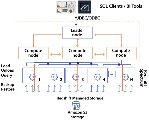
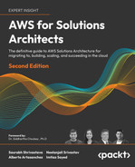
Figure 11.1: Redshift cluster architecture

As shown in the preceding diagram, Redshift has one leader node and multiple compute nodes. The leader node is required and automatically provisioned in every Redshift cluster, but customers are not charged for the leader node. The leader is responsible for being the user’s JDBC/ODBC entry point to the cluster, storing metadata, compiling queries, and coordinating parallel SQL processing.

When the leader node receives your query, it converts the query into C++ code, which is compiled and sent down to all the compute nodes by the leader node. Behind the leader node are the compute nodes responsible for query execution and data manipulation. Compute nodes operate in parallel. Redshift clusters can be as small as one node that houses both the leader node and the compute node or as large as 128 compute nodes.

Next, these compute nodes also talk to other AWS services, primarily S3. You ingest data from S3 and unload data to S3. AWS continuously backs up your cluster to S3, all happening in the background and in parallel. Compute nodes also interact with Spectrum nodes, a Redshift feature that allows a Redshift cluster to query external data like that in an S3 data lake.

The following are the major responsibilities of Redshift components:

• Leader node:
  • SQL endpoint
  • Stores metadata
  • Coordinates parallel SQL processing and ML optimizations
  • No cost to use for clusters
• Compute nodes:
  • Local, columnar storage
  • Executes queries in parallel
  • Load, unload, backup, and restore from S3
• Amazon Redshift Spectrum nodes:
  • Redshift Spectrum nodes enable you to expand your Redshift analytics capabilities beyond the data warehouse by querying large volumes of unstructured data stored in your Amazon S3 data lake

In Redshift, compute nodes are divided into smaller units called “slices,” which act like virtual compute nodes. Each slice is allocated a certain amount of memory and disk space from the physical compute node. The leader node is responsible for processing a portion of the workload assigned to the compute node and distributing data to the slices. It also assigns tasks related to queries and other database operations to the slices. The slices work in parallel and only operate on their assigned data, but they can request data from other slices if needed to complete their tasks. The number of slices per node varies depending on the instance type, with small instance types having 2 slices per node and large instance types having 16 slices per node.

In Redshift, data sharing enables you to share data with other Amazon Redshift clusters and databases, as well as with Athena and Amazon QuickSight. This is useful if you have multiple Amazon Redshift clusters that need to access the same data, or if you want to use Athena or QuickSight to analyze data stored in an Amazon Redshift cluster.

You can share data in Amazon Redshift by creating a read-only external schema that points to the data, and then grant access to that schema to other Amazon Redshift clusters or databases. This allows the other clusters or databases to query the data as if it were stored locally.

Redshift supports materialized views (MVs). MVs are pre-computed results of a SELECT query that are stored in a table. MVs can be used to speed up query performance by storing the results of a SELECT query in a table so that the SELECT query can be run faster the next time it is needed. MVs are especially useful when the data used in the SELECT query is not changing frequently because the results of the SELECT query can be refreshed periodically to ensure that the data in the MV is up to date. Let’s learn about the Redshift instance types.

Redshift instance types

Amazon Redshift offers a variety of node types to support different workloads and performance requirements:

• RA3 node types: These are the latest generation of Amazon Redshift node types, and they offer the ability to scale compute and storage independently. RA3 node types are suitable for workloads that require both high-performance computing and high-capacity storage. They are available in both single-node and multi-node configurations. The RA3 node is a technology that allows independent computing and storage scaling. It utilizes Redshift Managed Storage (RMS) as its resilient storage layer, providing virtually limitless storage capacity where data is committed back to Amazon S3. This allows for new functionalities, such as data sharing, where RMS can be used as shared storage across numerous clusters.
• Dense Compute (DC) node types: These node types are designed for high-performance computing and are suitable for workloads that require fast query performance, such as data warehousing and business intelligence. DC node types offer a balance of CPU, memory, and storage, and are available in both single-node and multi-node configurations.

The following table shows details of the latest Redshift instance types:

Table 11.1: Comparison between Redshift instance types

Redshift launched with Dense Storage (DS) nodes, but those are on the path to deprecation now. DS nodes are optimized for high-capacity storage and are suitable for workloads that require large amounts of data, such as data lakes and big data analytics.

A Redshift cluster can have up to 128 ra3.16xlarge nodes, which is 16 petabytes of managed storage. When you have a data warehouse storing such a massive amount of data, you want to make sure it can scale and provide query performance. The following are some key Redshift features:

• Redshift Concurrency Scaling – Redshift Concurrency Scaling is a feature that automatically adjusts cluster capacity to handle unexpected spikes in user demand, allowing thousands of users to work simultaneously without any degradation in performance.
• Advanced Query Accelerator (AQUA) – A hardware-level cache that takes performance to the next level, accelerating query speed up to 10x.
• Redshift federated queries – Allow you to combine data from multiple data sources and query it as if it were all stored in a single Amazon Redshift database. This is useful if you have data stored in different data stores, such as Amazon S3, Amazon RDS, or even other Amazon Redshift clusters, and you want to analyze the data using Amazon Redshift.
• Automatic workload management (WLM) – Provides fine-grained control like query monitoring rules to promote or demote query priorities at execution time based on certain runtime metrics, for example, the queue wait, execution time, CPU usage, and so on.
• Elastic resize – Enables the in-place addition or removal of nodes to/from existing clusters within a few minutes.
• Auto-vacuum – Monitors changes to your workload and automatically reclaims disk space occupied by rows affected by UPDATE and DELETE operations.
• Redshift Advisor – Continuously monitors and automatically provides optimization recommendations.
• Redshift Query Editor – Web-based query interface to run single SQL statement queries in an Amazon Redshift cluster directly from the AWS Management Console.
• Redshift ML – Amazon Redshift ML is a feature of Amazon Redshift that allows you to use SQL to build and train ML models on data stored in an Amazon Redshift cluster. With Redshift ML, you can use standard SQL statements to create and train ML models without having to learn a new programming language or use specialized ML libraries.

As you expand analytics throughout organizations, you need to make data easily and rapidly accessible to line of business users with little or no knowledge about data warehouse management. You do not want to consider selecting instances, sizing, scaling, and tuning the data warehouse. Instead, you want a simplified, self-service, automated data warehouse experience that allows them to focus on rapidly building business applications. To address these challenges, AWS launched Amazon Redshift Serverless at re:Invent 2021. You can go to the Amazon Redshift console and enable a serverless endpoint for your AWS account. You can get started with queries from the query editor tool that comes out of the box with Amazon Redshift or connect from your favorite tool via JDBC/ODBC or data API. You don’t need to select node types to specify the node or do another manual configuration such as workload management, scaling configurations, and so on.

Amazon Redshift and Amazon Redshift Serverless are both fully managed data warehousing solutions. However, there are some key differences between the two offerings that you should consider when deciding which one is right for your use case. One of the main differences between Redshift and Redshift Serverless is the way they are priced. Amazon Redshift is priced based on the number and type of nodes in your cluster, as well as the amount of data you store and the amount of data you query. You pay a fixed hourly rate for each node in your cluster, and you can scale the number of nodes up or down as needed to meet changing workload demands.

In contrast, Redshift Serverless is priced based on the amount of data you store and the number of queries you run. You don’t need to provision any nodes or worry about scaling the number of nodes up or down. Instead, Amazon Redshift Serverless automatically scales the number of compute resources needed to run your queries based on the workload demand. You only pay for the resources you use, and you can pause and resume your cluster as needed to save costs.

Another key difference between the two offerings is the way they handle concurrency and workload management. Amazon Redshift uses a leader node to manage the workload and distribute tasks to compute nodes, which can be scaled up or down as needed. Amazon Redshift Serverless, on the other hand, uses a shared pool of resources to run queries, and automatically allocates more resources as needed to handle increased concurrency and workload demands.

In general, Amazon Redshift is a good choice if you have a high-concurrency workload that requires fast query performance and you want to be able to scale the number of compute resources up or down as needed. Amazon Redshift Serverless is a good choice if you have a lower-concurrency workload that varies over time, and you want a more cost-effective solution that automatically scales compute resources as needed. Let’s look at some tips and tricks to optimize a Redshift workload.

Optimizing Redshift workloads

There are several strategies you can use to optimize the performance of your Amazon Redshift workload:

• Use the right node type: Choose the right node type for your workload based on the performance and storage requirements of your queries. Amazon Redshift offers a variety of node types, including DC, DS, memory-optimized, and RA3, which are optimized for different workloads.
• Use columnar storage: Amazon Redshift stores data using a columnar storage layout, which is optimized for data warehousing workloads. To get the best performance from Amazon Redshift, make sure to design your tables using a columnar layout and use data types that are optimized for columnar storage.
• Use sort keys and distribution keys: Sort keys and distribution keys are used to optimize the way data is stored and queried in Amazon Redshift. Use sort keys to order the data in each block of data stored on a node, and use distribution keys to distribute data evenly across nodes. This can help to improve query performance by reducing the amount of data that needs to be read and processed.
• Use Materialized Views (MVs): MVs are pre-computed results of a SELECT query that are stored in a table. MVs can be used to speed up query performance by storing the results of a SELECT query in a table so that the SELECT query can be run faster the next time it is needed.
• Use query optimization techniques: There are several techniques you can use to optimize the performance of your queries in Amazon Redshift, including using the EXPLAIN command to understand query execution plans, using the right join type, and minimizing the use of functions and expressions in your queries.
• Use Redshift Spectrum: Redshift Spectrum is an Amazon Redshift feature that enables you to query data stored in Amazon S3 using SQL, without having to load the data into an Amazon Redshift cluster. This can be a cost-effective way to query large amounts of data and can also help to improve query performance by offloading data processing to the scale-out architecture of Amazon S3.

In this section, you learned about the high-level architecture and key features of Redshift, which gave you a pointer to start your learning. Redshift is a very vast topic that warrants an entire book in itself. You can refer to Amazon Redshift Cookbook to dive deeper into Redshift – https://www.amazon.com/dp/1800569688/.

While Redshift is a relational engine and operates on structured data, you must be curious about getting insight from other semi-structured data coming in at a high velocity and volume. To help mine this data without hassle, AWS provides Amazon Athena. This allows you to query data directly from S3.

Querying your data lake in AWS with Amazon Athena

Water, water everywhere, and not a drop to drink… This may be the feeling you get in today’s enterprise environments. We are producing data at an exponential rate, but it is sometimes difficult to find a way to analyze this data and gain insights from it. Some of the data that we are generating at a prodigious rate is of the following types:

• Application logging
• Clickstream data
• Surveillance video
• Smart and IoT devices
• Commercial transactions

Often, this data is captured without analysis or is at least not analyzed to the fullest extent. Analyzing this data properly can translate into the following:

• Increased sales
• Cross-selling opportunities
• Avoiding downtime and errors before they occur
• Serving customer bases more efficiently

Previously, one stumbling block to analyzing this data was that much of this information resided in flat files. To analyze them, we had to ingest these files into a database to be able to perform analytics. Amazon Athena allows you to analyze these files without going through an Extract, Transform, Load (ETL) process.

Amazon Athena treats any file like a database table and allows you to run SELECT statement queries. Amazon Athena also now supports insert and update statements. The ACID transactions in Athena enable various operations like write, delete, and update to be performed on Athena’s SQL data manipulation language (DML).

You can greatly increase processing speeds and lower costs by running queries directly on a file without first performing ETL on them or loading them into a database. Amazon Athena enables you to run standard SQL queries to analyze and explore Amazon S3 objects. Amazon Athena is serverless. In other words, there are no servers to manage.

Amazon Athena is extremely simple to use. All you need to do is this:

1. Identify the object you want to query in Amazon S3.
2. Define the schema for the object.
3. Query the object with standard SQL.

Depending on the size and format of the file, query results can take a few seconds. As we will see later, a few optimizations can reduce query time as files get bigger.

Amazon Athena can be integrated with the AWS Glue Data Catalog. Doing so enables the creation of a unified metadata repository across services. You learned about Glue in Chapter 10, Big Data and Streaming Data Processing in AWS. AWS Glue crawls data sources, discovering schemas and populating the AWS Glue Data Catalog with any changes that have occurred since the last crawl, including new tables, modifications to existing tables, and new partition definitions, while maintaining schema versioning.

Let’s get even deeper into the power and features of Amazon Athena and how it integrates with other AWS services.

Deep-diving into Amazon Athena

As mentioned previously, Amazon Athena is quite flexible and can handle simple and complex database queries using standard SQL. It supports joins and arrays. It can use a wide variety of file formats, including these:

• CSV
• JSON
• ORC
• Avro
• Parquet

It also supports other formats, but these are the most common. In some cases, the files you are using have already been created, and you may have little flexibility regarding the format of these files. But for the cases where you can specify the file format, it’s important to understand the advantages and disadvantages of these formats. In other cases, converting the files into another format may even make sense before using Amazon Athena. Let’s take a quick look at these formats and understand when to use them.

CSV files

A Comma-Separated Value (CSV) file is a file where a comma separator delineates each value, and a return character delineates each record or row. Remember that the separator does not necessarily have to be a comma. Other common delimiters are tabs and the pipe character (|).

JSON files

JavaScript Object Notation (JSON) is an open-standard file format. One of its advantages is that it’s somewhat simple to read, mainly when it’s indented and formatted. It’s a replacement for the Extensible Markup Language (XML) file format, which, while similar, is more difficult to read. It consists of a series of potentially nested attribute-value pairs.

JSON is a language-agnostic data format. It was initially used with JavaScript, but quite a few programming languages now provide native support for it or provide libraries to create and parse JSON-formatted data.

ORC files

The Optimized Row Columnar (ORC) file format provides a practical method for storing files. It was initially designed under the Apache Hive and Hadoop project and was created to overcome other file formats’ issues and limitations. ORC files provide better performance when compared to uncompressed formats for reading, writing, and processing data.

Apache Avro files

Apache Avro is an open-source file format used to serialize data. It was originally designed for the Apache Hadoop project.

Apache Avro uses JSON format to define data schemas, allowing users of files to read and interpret them easily. However, the data is persisted in binary format, which has efficient and compact storage. An Avro file can use markers to divide big datasets into smaller files to simplify parallel processing. Some consumer services have a code generator that processes the file schema to generate code that enables access. Apache Avro doesn’t need to do this, making it suitable for scripting languages.

An essential Avro characteristic is its support for dynamic data schemas that can be modified over time. Avro can process schema changes such as empty, new, and modified fields. Because of this, old scripts can process new data, and new scripts can process old data. Avro has APIs for the following, among others:

• Python
• Go
• Ruby
• Java
• C
• C++

Avro-formatted data can flow from one program to another even if the programs are written in different languages.

Apache Parquet files

Just because we are listing Parquet files at the end, don’t assume they will be ignored. Parquet is an immensely popular format to use in combination with Amazon Athena.

Apache Parquet is another quite popular open-source file format. Apache Parquet has an efficient and performant design. It stores file contents in a flat columnar storage format. Contrast this storage method with the row-based approach used by comma- and tab-delimited files such as CSV and TSV.

Parquet is powered by an elegant assembly and shredding algorithm that is more efficient than simply flattening nested namespaces. Apache Parquet is well suited to operating on complex data at scale by using efficient data compression.

This method is ideal for queries that require reading a few columns from a table with many columns. Apache Parquet can easily locate and scan only those columns, significantly reducing the traffic required to retrieve data.

In general, columnar storage and Apache Parquet deliver higher efficiency than a row-based approach such as CSV. While performing reads, a columnar storage method will skip over non-relevant columns and rows efficiently. Aggregation queries using this approach take less time than row-oriented databases. This results in lower billing and higher performance for data access.

Apache Parquet supports complex nested data structures. Parquet files are ideal for queries retrieving large amounts of data, and can handle files that contain gigabytes of data without much difficulty.

Apache Parquet is built to support a variety of encoding and compression algorithms. Parquet is well suited to situations where columns have similar data types. This can make accessing and scanning files quite efficient. Apache Parquet works with various codes, enabling the compression of files in various ways.

In addition to Amazon Athena, Apache Parquet works with serverless technologies such as Google BigQuery, Google Dataproc, and Amazon Redshift Spectrum.

Understanding how Amazon Athena works

Amazon Athena was initially intended to work with data stored in Amazon S3. As we have seen, it can now work with other source types as well.

This feature of Amazon Athena is a game-changer. You can combine disparate data sources just as easily as if they all had the same format. This enables you to join a JSON file with a CSV file or a DynamoDB table with an Amazon Redshift table.

Previously, if you wanted to combine this data, performing a combination programmatically would invariably translate into a long development cycle and more than likely not scale well when using large datasets.

Now all you have to do is write an SQL query that combines the two data sources. Due to the underlying technology, this technique will scale well, even when querying terabytes and petabytes of data.

Data scientists and data analysts will be able to work at a speed that would have been impossible just a few years ago.

Under the hood, Amazon Athena leverages Presto. Presto is an open-source SQL query engine. Queries in Amazon Athena can be quite complex and can use joins, window functions, and complex data types. Amazon Athena is an excellent way to implement a schema-on-read strategy. A schema-on-read strategy enables you to project a schema onto existing data during query execution. Doing this eliminates the need to load or transform the data before it is queried, and instead, it can be queried wherever it lives.

Presto, also called PrestoDB, is an open-source, distributed SQL query engine with a design that can support, in a scalable fashion, queries on files and other kinds of data sources. Some of the sources that are supported are listed here:

• Amazon S3
• Hadoop Distributed File System (HDFS)
• MongoDB
• Cassandra

It also supports traditional relational databases, such as these:

• MySQL
• Microsoft SQL Server
• Amazon Redshift
• PostgreSQL
• Teradata

It can handle petabyte-sized files. Presto can access data in place without the need to copy the data. Queries can execute in parallel in memory (without having access to secondary storage) and return results in seconds.

You might want to use Athena with SQL queries on a Relational Database Management System (RDBMS) database if you want to perform ad hoc queries on the data without having to load it into a data warehouse first. With Athena, you can query the data in place in S3, which can be faster and more flexible than loading the data into a data warehouse and then querying it.

Initially, Amazon Athena only leveraged Presto to access Amazon S3 files, but Amazon now offers Amazon Athena Federated Query. We will learn more about it in the next section.

Using Amazon Athena Federated Query

Unless your organization has specific requirements, it’s likely that you store data in various storage types, selecting the most appropriate storage type based on its purpose. For example, you may choose graph databases when they are the best fit, relational databases for certain use cases, and S3 object storage or Hadoop HDFS when they are the most suitable. Amazon Neptune (a graph database) may be the best choice if you are building a social network application. Or, if you are building an application that requires a flexible schema, Amazon DynamoDB may be a solid choice. AWS offers many different types of persistence solutions, such as these:

• Relational database services
• Key-value database services
• Document database services
• In-memory database services
• Search database services
• Graph database services
• Time-series database services
• Ledger databases database services
• Plain object data stores (such as Amazon S3)

The reason it offers all these kinds of persistence storage systems is to accommodate the different needs that different services can have. Sometimes, corporations have mandates to only use a certain database or certain file storage, but even in such cases, there will probably be “fit-for-purpose” choices for different cases (a graph database, a NoSQL database, file storage, and more). As a design principle, this pattern is recommended and encouraged. It’s about following the principle of “choosing the right tool for a particular job.”

However, this plethora of choices poses a problem. As the number of different types of storage increases, running analytics and building applications across these data sources becomes more and more challenging. Overcoming this challenge is exactly what Amazon Athena Federated Query can help alleviate.

Amazon Athena Federated Query empowers data scientists, data analysts, and application engineers to run SQL queries across multiple data stores regardless of the data source type.

Before Amazon Athena Federated Query or any other way to run federated queries, we had to execute various queries across systems and merge, filter, and assemble the results once the individual queries were run.

Constructing these data pipelines to process data across data sources creates bottlenecks and requires developing customized solutions that can validate the consistency and accuracy of the data. When source systems are changed, the data pipelines must also be changed. Using query federation in Athena reduces these complexities by enabling users to run queries that retrieve data in situ no matter where it resides. Users can use standard SQL statements to merge data across disparate data sources in a performant manner. Users can also schedule SQL queries to retrieve data and store the results in Amazon S3.

This is a complicated and slow way to put together results.

Amazon Athena Federated Query allows you to execute a single SQL query across data stores, greatly simplifying your code while at the same time getting those results a lot faster, thanks to a series of optimizations provided by Amazon Athena Federated Query.

The following diagram illustrates how Amazon Athena can be leveraged against a variety of data source types (it only shows some of the data source types supported):

As we can see from the preceding figure, Amazon Athena Federated Query can handle a variety of disparate data sources and enables users to combine and join them with ease.

Data source connectors

Executing an SQL query against a new data source can be done simply by adding the data source to the Amazon Athena registry. The choice between the Athena registry and the Glue Catalog depends on your specific requirements and the complexity of your data and metadata management needs. If you need a simple and lightweight metadata store, the Athena registry may be sufficient. If you need a more feature-rich and powerful metadata store, the Glue Catalog may be a better choice.

Amazon Athena has open-source connectors. Additionally, AWS allows you to write your own custom connectors if there isn’t a suitable one. The connector performs the following functions:

• Manages metadata information
• Determines the parts of a data source that are required to be scanned, accessed, and filtered
• Manages query optimization and query parallelism

Amazon Athena can do this for any data source type with an Amazon Athena data source connector. These connectors run on AWS Lambda. AWS provides data source connectors for the following:

• Amazon DocumentDB
• Amazon DynamoDB
• Amazon Redshift
• Any JDBC-compliant RDBMS (such as MySQL, PostgreSQL, and Oracle)
• Apache HBase
• AWS CloudWatch Metrics
• Amazon CloudWatch Logs
• And more...

These connectors can be used to run federated standard SQL queries spanning multiple data sources, all inside of the Amazon Athena console or within your code.

Amazon Athena allows you to use custom connectors to query data stored in data sources that are not natively supported by Athena. Custom connectors are implemented using the Apache Calcite framework and allow you to connect to virtually any data source that has a JDBC driver.

To use a custom connector with Athena, you first need to create a custom data source definition using the CREATE DATA SOURCE command. This definition specifies the JDBC driver and connection information for the data source, as well as the schema and table definitions for the data. Once the custom data source is defined, you can use SQL to query the data as if it were a regular Athena table. Athena will use the custom connector to connect to the data source and execute the SQL query and will return the results to the client.

The Amazon Athena Query Federation SDK expands on the advantage of federated querying beyond the “out-of-the-box” connectors that come with AWS. By writing a hundred lines of code or less, you can create connectors to custom data sources and enable the rest of your organization to use this custom data. Once a new connector is registered, Amazon Athena can use the new connector to access databases, schemas, tables, and columns in this data source.

Let’s now learn about another powerful Athena feature – Amazon Athena workgroups.

Learning about Amazon Athena workgroups

Another new feature that comes with Amazon Athena is the concept of workgroups. Workgroups enable administrators to give different groups of users different access to databases, tables, and other Athena resources. It also enables you to establish limits on how much data a query or a whole workgroup can access, and provides the ability to track costs. Since workgroups act like any other resource in AWS, resource-level identity-based policies can be set up to control access to individual workgroups.

Workgroups can be integrated with SNS and CloudWatch as well. If query metrics are turned on, these metrics can be published to CloudWatch. Additionally, alarms can be created for certain workgroup users if their usage goes above a pre-established threshold.

By default, Amazon Athena queries run in the default primary workgroup. AWS administrators can add new workgroups and then run separate workloads in each workgroup. A common use case is to use workgroups to separate audiences, such as users who will run ad hoc queries and users who will run pre-canned reports. Each workgroup can then be associated with a specific location. Any queries associated with an individual workgroup will have their results stored in the assigned location. Following this paradigm ensures that only users that should be able to access certain data can access that data.

Another way to restrict access is by applying different encryption keys to the output files depending on the workgroup.

A task that workgroups greatly simplifies is the onboarding of new users. You can override the client-side settings and apply a predefined configuration for all the queries executed in a workgroup. Users within a workgroup do not have to configure where their queries will be stored or specify encryption keys for the S3 buckets. Instead, the values defined at the workgroup level will be used as a default.

Also, each workgroup keeps a separate history of all executed queries and any queries that have been saved, making troubleshooting easier.

Optimizing Amazon Athena

As with any SQL operation, you can take steps to optimize the performance of your queries and inserts. As with traditional databases, optimizing your data access performance usually comes at the expense of data ingestion and vice versa.

Let’s look at some tips that you can use to increase and optimize performance.

Optimization of data partitions

One way to improve performance is to break up files into smaller files called partitions. A common partition scheme breaks up a file by using a divider that occurs with some regularity in data. Some examples follow:

• Country
• Region
• Date
• Product

Partitions operate as virtual columns and reduce the amount of data that needs to be read for each query. Partitions are normally defined at the time a table or file is created.

Amazon Athena can use Apache Hive partitions. Hive partitions use this name convention:

s3://BucketName/TablePath/<PARTITION_COLUMN_NAME>=<VALUE>/<PARTITION_COLUMN_NAME>=<VALUE>/

When this format is used, the MSCK REPAIR command can be used to add additional partitions automatically.

Partitions are not restricted to a single column. Multiple columns can be used to partition data. Alternatively, you can divide a single field to create a hierarchy of partitions. For example, it is not uncommon to divide a date into three pieces and partition the data using the year, the month, and the day.

An example of partitions using this scheme may look like this:

s3://a-simple-examples/data/parquet/year=2000/month=1/day=1/
s3://a-simple-examples/data/parquet/year=2000/month=2/day=1/
s3://a-simple-examples/data/parquet/year=2000/month=3/day=1/
s3://a-simple-examples/data/parquet/year=2000/month=4/day=1/

So, which column would be the best to partition files and are there any best practices for partitioning? Consider the following:

• Any column normally used to filter data is probably a good partition candidate.
• Don’t over-partition. Suppose the number of partitions is too high; the retrieval overhead increases. If the partitions are too small, this prevents any benefit from partitioning the data.

It is also important to partition smartly and try to choose a value that is evenly distributed as your partition key. For example, if your data involves election ballots, it may initially seem like a good idea to use them as your partition of the candidates in the election. But what if one or two candidates take most of the votes? Your partitions will be heavily skewed toward those candidates, and your performance will suffer.

Data bucketing

Another scheme to partition data is to use buckets within a single partition. When using bucketing, a column or multiple columns are used to group rows together and “bucket” or categorize them. The best columns to use for bucketing are columns that will often be used to filter the data. So, when queries use these columns as filters, not as much data will need to be scanned and read when performing these queries.

Another characteristic that makes a column a good candidate for bucketing is high cardinality. In other words, you want to use columns that have a large number of unique values. So, primary key columns are ideal bucketing columns.

Amazon Athena offers the CLUSTERED BY clause to simplify which columns will be bucketed during table creation. An example of a table creation statement using this clause follows:

CREATE EXTERNAL TABLE employee (
id string,
name string,
salary double,
address string,
timestamp bigint)
PARTITIONED BY (
timestamp string,
department string)
CLUSTERED BY (
id,
timestamp)
INTO 50 BUCKETS

You can learn more about data partitioning in Athena by visiting AWS document here - https://docs.aws.amazon.com/athena/latest/ug/partitions.html.

File compression

Intuitively, queries can be sped up by using compression. When files are compressed, not as much data needs to be read, and the decompression overhead is not high enough to negate its benefits. Also, when going across the wire, a smaller file will take less time to get through the network than a bigger file. Finally, faster reads and transmission over the network will result in less spending, which, when you multiply these by hundreds and thousands of queries, will result in real savings over time.

Compression offers the highest benefits when files are of a certain size. The optimal file size is around 200 megabytes to 1 gigabyte. Smaller files translate into multiple files being able to be processed simultaneously, taking advantage of the parallelism available with Amazon Athena. If there is only one file, only one reader can be used on the file while other readers sit idle.

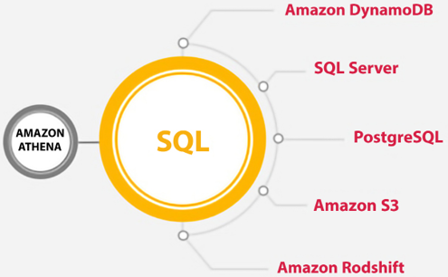
One simple way to achieve compression is to utilize Apache Parquet or Apache ORC format. Files in these formats can be easily split, and these formats are compressed by default. Two compression formats are often combined with Parquet and ORC to improve performance further. These compression formats are Gzip and Bzip2. The following chart shows how these compression formats compare with other popular compression algorithms:

Figure 11.3: Compression formats

Each format offers different advantages. As shown in the figure, Gzip and Snappy files cannot be split. Bzip2 can be split. LZO can only be split in special cases. Bzip2 provides the highest compression level, and LZO and Snappy provide the fastest compression speed.

Let’s continue learning about other ways to optimize Amazon Athena. Another thing to do is to ensure the optimal file size.

File size optimization

As we have seen in quite a few examples in this book, one of the game-changing characteristics of the cloud is its elasticity. This elasticity enables us to run queries in parallel easily and efficiently. File formats that allow file splitting assist in this parallelization process. If files are too big or are not split, too many readers will be idle, and parallelization will not occur. On the flip side, files that are too small (generally in the range of 128 megabytes or less) will incur additional overhead with the following operations, to name a few:

• Opening files
• Listing directories
• Reading file object metadata
• Reading file headers
• Reading compression dictionaries

So, just as it’s a good idea to split bigger files to increase parallelism, it is recommended to consolidate smaller files. Amazon EMR has a utility called S3DistCP that can be used to merge smaller files into larger ones. S3DistCP can also be used to transfer large files efficiently from HDFS to Amazon S3 and vice versa, as well as from one S3 bucket to another. Here is an example of how to use S3DistCP to copy data from an S3 bucket to an EMR cluster:

aws s3-dist-cp --src s3://sa-book-source-bucket/path/to/data/ 
             --dest hdfs:///path/to/destination/sa-book/ 
             --s3-client-region us-east-2 
             --s3-client-endpoint s3.us-east-2.amazonaws.com 
             --src-pattern '*.csv' 
             --group-by '.*(part|PARTS)..*'

The example above copies all .csv files from the sa-book-source-bucket S3 bucket to the /path/to/destination/sa-book/ directory on the EMR cluster. The --src-pattern option specifies a regular expression to match the files that should be copied, and the --group-by option specifies a regular expression to group the files into larger blocks for more efficient transfer.

The --s3-client-region and --s3-client-endpoint options specify the region and endpoint of the S3 bucket.

S3DistCP has many other options that you can use to customize the data transfer process, such as options to specify the number of mappers to use, the maximum number of retries, and the maximum number of concurrent connections. You can find more information about these options in the S3DistCP documentation – https://aws.amazon.com/fr/blogs/big-data/seven-tips-for-using-s3distcp-on-amazon-emr-to-move-data-efficiently-between-hdfs-and-amazon-s3/.

Columnar data store generation optimization

As mentioned earlier, Apache Parquet and Apache ORC are popular columnar data store formats. The formats efficiently compress data by leveraging the following:

• Columnar-wise compression scheme
• Datatype-based compression
• Predicate pushdown
• File splitting

A way to further optimize compression is to fine-tune the file’s block size or stripe size. Having bigger block and stripe sizes enables us to store more rows per block. The default Apache Parquet block size is 120 megabytes, and the default Apache ORC stripe size is 64 megabytes. A larger block size is recommended for tables with a high number of columns. This ensures that each column has a reasonable size that enables efficient sequential I/O.

When datasets are 10 gigabytes or less, using the default compression algorithm that comes with Parquet and ORC is enough to have decent performance, but for datasets bigger than that, it’s not a bad idea to use other compression algorithms with Parquet and ORC, such as Gzip.

Yet another parameter that can be customized is the type of compression algorithm used on the storage data blocks. The Parquet format, by default, uses Snappy, but it also supports these other formats:

• Gzip
• LZO
• No compression

The ORC format uses Zlib compression by default, but it also supports the following:

• Snappy
• No compression

The recommended way to choose a compression algorithm is to use the default algorithm. No further optimization is needed if the performance is good enough for your use case. If it’s not, try the other supported formats to see if they deliver better results.

Column selection

An obvious way to reduce network traffic is to ensure that only the required columns are included in each query. Therefore, it is not recommended to use the following syntax unless your application requires that every single column in a table be used. And even if that’s true today, it may not be true tomorrow. If additional columns are later added to the table schema, they may not be required for existing queries. Take this, for instance:

Select * from the table

Instead of that, use this:

select column1, column2, column3 from table

By explicitly naming columns instead of using the star operator, we reduce the number of columns that get passed back and lower the number of bytes that need to be pushed across the wire.

Let’s now learn about yet another way to optimize our use of Amazon Athena and explore the concept of predicate pushdown.

Predicate pushdown

The core concept behind predicate pushdown (also referred to as predicate filtering) is that specific sections of an SQL query (a predicate) can be “pushed down” to the location where the data exists. Performing this optimization can help reduce (often drastically) the time it takes a query to respond by filtering out results earlier in the process. Sometimes, predicate pushdown is achieved by filtering data in situ before transferring it over the network or loading it into memory.

The ORC and the Parquet formats support predicate pushdown. These formats have data blocks representing column values. In each block, statistics are stored for the data held in the block. Two examples of the statistics stored are the minimum and the maximum value. When a query is run, these statistics are read before the rest of the block and, depending on the statistics, it is determined whether the complete block should be read.

To take maximum advantage of predicate pushdown, it is recommended to identify the column that will be used the most when executing queries before writing to disk and to sort by that column. Let’s look at a quick example to drive the point home.

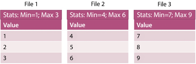
In the preceding example, there are three files. As you can tell, the data is already sorted using the value stored in the column labeled Value. Let’s say we want to run the following query:

select * from Table where Value = 5

As mentioned before, we can look at the statistics first and observe that the first file’s maximum value is 3, so we can skip that file. In the second file, we see that our key (Value = 5) falls within the range of values in the file. We would then read this file. Since the maximum value of the second file is greater than the value of our key, we don’t need to read any more files after reading the second file.

Predicate pushdown is used to reduce the amount of data that needs to be scanned when executing a query in Amazon Athena. Predicate pushdown works by pushing down filtering conditions (predicates) to the data sources being queried, so that the data sources can filter the data before returning it to Athena. This can significantly reduce the amount of data that needs to be scanned and processed by Athena, which can improve query performance and reduce costs. You should use it whenever you have a query that has predicates that can be applied to the data sources being queried.

ORDER BY clause optimization

Due to how sorting works, when we invoke a query containing an ORDER BY clause, it needs to be handled by a single worker thread. This can cause query slowdown and even failure. There are several strategies you can use to optimize the performance of the ORDER BY clause in Athena:

• Use a sort key: If you have a large table that you frequently need to sort, you can improve query performance by using a sort key. A sort key is a column or set of columns that is used to order the data in the table. When you use a sort key, Athena stores the data in the table in a sorted order, which can significantly reduce the time it takes to sort the data when you run a query.
• Use a LIMIT clause: If you only need the top N rows of a query, you can use the LIMIT clause to limit the number of rows returned. This can reduce the amount of data that needs to be sorted and returned, which can improve query performance.
• Use a computed column: If you frequently need to sort a table based on a derived value, you can create a computed column that contains the derived value and use the computed column in the ORDER BY clause.

Join optimization

Table joins can be an expensive operation. Whenever possible, they should be avoided. In some cases, it makes sense to “pre-join” tables and merge two tables into a single table to improve performance when queries are executed later.

That is not always possible or efficient. Another way to optimize joins is to ensure that larger tables are always on the left side of the join, and the smaller tables are on the right-hand side. When Amazon Athena runs a query with a join clause, the right-hand side tables are delegated to worker nodes, bringing these tables into memory, and the table on the left is then streamed to perform the join. This approach will use a smaller amount of memory, and the query performs better.

And now, yet another optimization will be explored by optimizing GROUP BY clauses.

Group by clause optimization

When a GROUP BY clause is present, the best practice is arranging the columns according to the highest cardinality. For example, if you have a dataset that contains data on ZIP codes and gender, it is recommended to write the query like this:

SELECT zip_code, gender, COUNT(*)FROM dataset GROUP BY zip_code, gender

This way is not recommended:

Select zip code, gender, count(*) from the dataset group by gender

This is because it is more likely that the ZIP code will have a higher cardinality (there will be more unique values) in that column.

Additionally, this is not always possible, but minimizing the number of columns in the select clause is recommended when a GROUP BY clause is present.

Approximate function use

Amazon Athena has a series of approximation functions. For example, there is an approximation function for the DISTINCT() function. If you don’t need an exact count, you can instead use APPROX_DISTINCT(), which may not return the exact number of distinct values for a column in a given table, but it will give a good approximation for many use cases.

For example, to get an approximation, you should not use this query:

Select DISTINCT(last_name) from employee

Instead, you should use this query:

Select APPROX_DISTINCT(last_name) from employee

This may be suitable for a given use case if an exact count is not required.

This concludes the optimization section for Amazon Athena. It is by no means a comprehensive list, but rather it is a list of the most common and practical optimization techniques that can be used to gain efficiency and increase query performance quickly.

You have now learned about Amazon Redshift and Amazon Athena. Let’s see some examples of when to use Athena and when to use Redshift Spectrum for querying data.

Using Amazon Athena versus Redshift Spectrum

Amazon Athena and Redshift Spectrum are two data querying services offered by AWS that allow users to analyze data stored in Amazon S3 using standard SQL.

Amazon Athena is a serverless interactive query service that quickly analyzes data in Amazon S3 using standard SQL. It allows users to analyze data directly from Amazon S3 without creating or managing any infrastructure. Athena is best suited for ad hoc querying and interactive analysis of large amounts of unstructured data that is stored in Amazon S3.

For example, imagine a marketing team needs to analyze customer behavior data stored in Amazon S3 to make informed decisions about their marketing campaigns. They can use Athena to query the data in S3, extract insights, and make informed decisions about how to improve their campaigns.

On the other hand, Amazon Redshift Spectrum (an extension of Amazon Redshift) allows users to analyze data stored in Amazon S3 with the same SQL interface used to analyze data in their Redshift cluster. It extends the querying capabilities of Redshift beyond the data stored in its own nodes to include data stored in S3.

Redshift Spectrum allows users to store data in S3 and query it as if it were in their Redshift cluster without loading or transforming the data. Redshift Spectrum is best suited for users who want to query large amounts of structured data stored in S3 and join it with data already stored in their Redshift cluster.

For example, a retail company might store its transactional data in Redshift and its historical data in S3. The company can use Redshift Spectrum to join its Redshift transactional data with its historical data in S3 to gain deeper insights into customer behavior.

In summary, Amazon Athena and Amazon Redshift Spectrum are both powerful data querying services that allow users to analyze data stored in Amazon S3 using standard SQL. The choice between the two largely depends on the type of data being analyzed and the specific use case. Athena is best suited for ad hoc querying and interactive analysis of large amounts of unstructured data, while Redshift Spectrum is best suited for querying large amounts of structured data stored in S3 and joining it with data already stored in a Redshift cluster.

As someone said, one picture is worth a thousand words, so it is always preferable to show data insight in a visual format using a business intelligence tool. AWS provides a cloud-based business intelligence tool called Amazon QuickSight, which visualizes your data and gets ML-based insights. Let’s learn more details about business intelligence in AWS.

Visualizing data with Amazon QuickSight

Data is an organizational asset that needs to be available easily and securely to anyone who needs access. Data is no longer solely the property of analysts and scientists. Presenting data simply and visually enables teams to make better and more informed decisions, improve efficiency, uncover new opportunities, and drive innovation.

Most traditional on-premises business intelligence solutions come with a client-server architecture and have minimum licensing requirements. To start with business intelligence tools, you must sign up for annual commitments around users or servers, requiring upfront investments. You will need to build extensive monitoring and management, infrastructure growth, patches for software, and periodic data backups to keep your systems in compliance. On top of that, if you want to deliver data and insights to your customers and other third parties, this usually requires separate systems and tools for each audience.

Amazon QuickSight is an AWS-provided cloud-native business intelligence SaaS solution, which means no servers or software to manage, and it can scale from single users to thousands of users under a pay-as-you-go model. With Amazon QuickSight, you can address a number of use cases to deliver insights for internal or external users. You can equip different lines of business with interactive dashboards and visualization and the ability to do ad hoc analysis. QuickSight gives you the ability to distribute highly formatted static reports to internal and external audiences by email. Further, you can enhance your end-user-facing products by embedding QuickSight visuals and dashboards into a website or application. There are several ways you can use QuickSight to analyze your data:

• Visualize and explore data: QuickSight allows you to create interactive visualizations and dashboards using your data. You can use a variety of chart types, including line graphs, bar charts, scatter plots, and heat maps, to explore and visualize your data. You can also use QuickSight’s built-in filters and drill-down capabilities to drill down into specific data points and get more detailed insights.
• Perform ad hoc analysis: QuickSight includes a powerful SQL-based analysis tool, Super-fast, Parallel, In-memory, Calculation Engine (SPICE), that allows you to perform ad hoc analysis on your data. You can use SPICE to write custom SQL queries and perform calculations on your data, and then visualize the results using QuickSight’s visualization tools. SPICE provides consistently fast performance for concurrent users automatically. You can import quite a bit of data into your SPICE datasets – up to 500 million rows each – and have as many SPICE datasets as you need. You can refresh each SPICE dataset up to 100 times daily without affecting performance or downtime.
• Use ML: QuickSight includes built-in ML capabilities that allow you to use predictive analytics to forecast future trends and patterns in your data. You can use QuickSight’s ML algorithms to create predictive models and generate forecasts, and then visualize the results using QuickSight’s visualization tools. QuickSight leverages ML to help users extract more value from their data with less effort. For instance, QuickSight Q is a natural language query (NLQ) engine that empowers users to ask questions about their data in plain English. QuickSight also generates insights using natural language processing (NLP) to make it easy for any user, no matter their data savviness, to understand the key highlights hidden in their data. QuickSight also provides 1-click forecasting and anomaly detection using an ML model.

Below is an example of a QuickSight dashboard that provides an analysis of home prices in the USA:

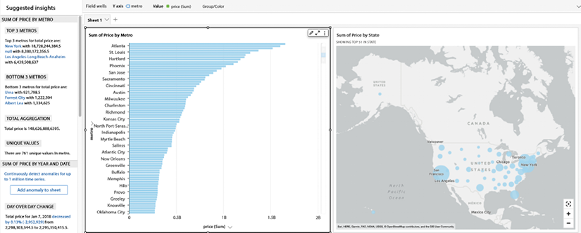
In the dashboard above, you can see that QuickSight is able to show a bar chart for median home prices in the US by city in the first chart, and a geolocation graph with bubbles in the second chart. Also, you can see ML-based insights on the left-hand side, which makes it easy to understand the graph in simple language.

Up until now, you have been learning about various AWS analytic services. Let’s use an example to put them together.

Putting AWS analytic services together

In the previous chapter, Chapter 10, Big Data and Streaming Data Processing in AWS, you learned about AWS ETL services such as EMR and Glue. In this chapter, let’s combine that with learning how to build a data processing pipeline. The following diagram shows a data processing and analytics architecture in AWS that applies various analytics services to build an end-to-end solution:

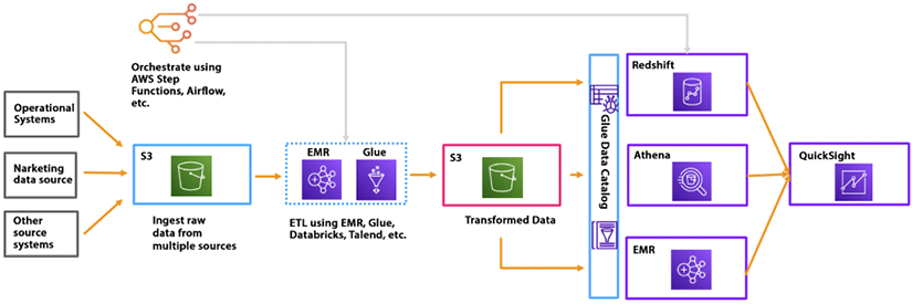
Figure 11.6: Data analytic architecture in AWS

As shown in the preceding diagram, data is ingested from various sources such as operational systems, marketing, and other systems in S3. You want to ingest data fast without losing it, so this data is collected in a raw format first. You can clean, process, and transform this data using an ETL platform such as EMR or Glue. Using the Apache Spark framework and writing data processing code from scratch is recommended when using Glue; otherwise, you can use EMR if you have Hadoop skill sets in your team. Transformed data is stored in another S3 bucket, which is further consumed by the data warehouse system in Redshift, the data processing system in EMR, and direct queries with Athena. Now, to visualize this data, you can connect QuickSight to any consumer.

The above is just one way to build a data pipeline; however, multiple ways are available to build data analytics architecture, such as data lakes, lake houses, data meshes, etc. You will learn about these architectures in Chapter 15, Data Lake Patterns – Integrating Your Data Across the Enterprise.

Summary

In this chapter, you learned how to query and visualize data in AWS. You started with learning about Amazon Redshift, your data warehouse in the cloud, before diving deeper into the Redshift architecture and learning about its key capabilities. Further, you learned about Amazon Athena, a powerful service that can “convert” any file into a database by allowing us to query and update the contents of that file by using the ubiquitous SQL syntax.

You then learned how we could add some governance to the process using Amazon Athena workgroups and how they can help us to control access to files by adding a level of security to the process. As you have learned throughout the book, there is not a single AWS service (or any other tool or product, for that matter) that is a silver bullet for solving all problems. Amazon Athena is no different, so you learned about some scenarios where Amazon Athena is an appropriate solution and other use cases where other AWS services, such as Amazon RDS, may be more appropriate for the job.

Further, you learned about the AWS-provided, cloud-native business intelligence service Amazon QuickSight, a powerful data visualization solution available under the SaaS model. You can achieve high performance in QuickSight using SPICE, its built-in caching engine. Finally, you combined multiple AWS analytics services and saw an example of an end-to-end data processing pipeline architecture in AWS.

In the next chapter, you will learn about making your data future-proof by applying AWS services to more advanced use cases in the areas of ML, IoT, blockchain, and even quantum computing.