7.9 CASE STUDY: HEDGING A FUTURE FIXED RATE ISSUANCE WITH AN INTEREST RATE SWAP
The aim of this case study is to illustrate the accounting treatment of hedges of highly expected future issuance of fixed rate debt with a forward starting interest rate swap. A forward starting swap is just a swap that starts sometime in the future. With this type of hedge the entity takes advantage of low interest rates prior to issuing the debt and/or does not want to take the risk of higher rates at issuance date.
7.9.1 Background Information
On 1 January 20X0, ABC (an entity with the EUR as functional currency) expected to issue a fixed rate bond on 15 July 20X0 with the following characteristics:
| Bond terms | |
| Expected issue date | 15 July 20X0 |
| Issuer | ABC |
| Issue proceeds | EUR 100 million (100% of notional) |
| Expected maturity | 3 years (15 July 20X3) |
| Notional | EUR 100 million |
| Coupon | Fixed, to be paid annually (30/360 basis) The coupon is expected to be set on the issue date at the EUR 3-year swap rate plus a 100 bps credit spread |
ABC was exposed to upward movements in the 3-year swap rate and to a widening of its own credit spread. ABC wanted to protect itself against potential increases in the 3-year interest rate until issuance date, by locking in the future coupon payment at 5.61% (assuming a spread of 100 basis points). Accordingly, on 1 January 20X0 ABC entered into a forward starting receive-fixed pay-floating interest rate swap with XYZ Bank with the following terms:
| Interest rate swap terms | |
| Trade date | 1 January 20X0 |
| Start date | 15 July 20X0 |
| Counterparties | ABC and XYZ Bank |
| Maturity | 3 years (15 July 20X3) |
| Notional | EUR 100 million |
| ABC pays | Euribor 12M annually (actual/360 basis) |
| ABC receives | 4.61% annually (30/360 basis) |
| Euribor fixing | Euribor is fixed 2 days prior to the commencement of the annual interest period |
| Initial fair value | Zero |
ABC planned to cancel the swap on the bond issue date (15 July 20X0). ABC designated the swap as the hedging instrument in a cash flow hedge of the highly expected issuance of the fixed rate bond. The effective amounts of the change in fair value of the swap until cancellation date would be recognised in equity. Following the bond issuance, the amounts accumulated in equity would be subsequently gradually recycled to profit or loss when the bond coupons impacted profit or loss. If the hedge was well constructed, the effective interest rate of the new bond would be close to the sum of the swap fixed rate and the credit spread, or 5.61% (=4.61% + 1%).
7.9.2 Hedging Relationship Documentation
ABC documented the hedging relationship as follows:
| Hedging relationship documentation | |
| Risk management objective and strategy for undertaking the hedge | The objective of the hedge is to eliminate the variability of the highly expected future cash outflows stemming from a planned issuance of a fixed rate bond by the entity. This hedging objective is consistent with the group's overall interest rate risk management strategy of managing the exposure to interest rate risk through the proportion of fixed and floating rate net debt in its total debt portfolio with interest rate swaps, caps and collars. Interest rate risk. The designated risk being hedged is the risk of changes in the EUR value of the hedged item attributable to changes in the Euribor interest rate. Fair value changes attributable to credit or other risks are not hedged in this relationship. Accordingly, the expected 100 basis points credit spread is excluded from the hedging relationship |
| Type of hedge | Cash flow hedge |
| Hedged item | The coupon cash flows of a 3-year fixed rate bond highly expected to be issued on 15 July 20X0 The issuance is highly expected to occur as it has been approved by the Board of Directors and a group of banks have been mandated |
| Hedging instrument | The interest rate swap with reference number 014569. The main terms of the swap are a EUR 100 million notional, a forward starting date on 15 July 20X0, a 3-year maturity, a 4.61% fixed rate to be received by the entity and a Euribor 12-month rate to be paid by the entity. The counterparty to the swap is XYZ Bank and the credit risk associated with this counterparty is considered to be very low. The interest rate swap is expected to be unwound on its forward starting date, which is expected to coincide with the bond's issue date |
| Hedge effectiveness assessment | See below |
7.9.3 Hedge Effectiveness Assessment
Hedge effectiveness will be assessed by comparing changes in the fair value of the hedging instrument to changes in the fair value of a hypothetical derivative. The terms of the hypothetical derivative are such that its fair value changes exactly offset the changes in fair value of the hedged item for the risk being hedged. The hypothetical derivative is a theoretical interest rate swap with no counterparty credit risk and with zero initial fair value, whose main terms are as follows:
| Hypothetical derivative terms | |
| Trade date | 1 January 20X0 |
| Start date | 15 July 20X0 |
| Counterparties | ABC and credit risk-free counterparty |
| Maturity | 3 years (15 July 20X3) |
| Notional | EUR 100 million |
| ABC pays | Euribor 12M annually, actual/360 basis |
| ABC receives | 4.615% annually, 30/360 basis |
| Euribor fixing | Euribor is fixed 2 days prior to the commencement of the annual interest period |
| Initial fair value | Zero |
The fixed rate of the hypothetical derivative is higher than that of the hedging instrument due to the absence of CVA in the former.
Changes in the fair value of the hedging instrument (i.e., the swap) will be recognised as follows:
- The effective part of the gain or loss on the hedging instrument will be recognised in the cash flow hedge reserve of equity. Following the bond issuance, the amounts accumulated in equity will be reclassified to profit or loss, on a linear basis, in the same period during which the hedged expected future cash flows affect profit or loss, adjusting interest expense.
- The ineffective part of the gain or loss on the hedging instrument will be recognised in profit or loss, as other financial income/expenses.
Hedge effectiveness will be assessed prospectively at hedging relationship inception, on an ongoing basis at least upon each reporting date and upon occurrence of a significant change in the circumstances affecting the hedge effectiveness requirements.
The hedging relationship will qualify for hedge accounting only if all the following criteria are met:
- The hedging relationship consists only of eligible hedge items and hedging instruments. The hedge item is eligible as it is a group of highly expected cash flows that will expose the entity to fair value risk, will affect profit or loss and is reliably measurable. The hedging instrument is eligible as it is a derivative that does not result in a net written option.
- At hedge inception there is a formal designation and documentation of the hedging relationship and the entity's risk management objective and strategy for undertaking the hedge.
- The hedging relationship is considered effective.
The hedging relationship will be considered effective if the following three requirements are met:
- There is an economic relationship between the hedged item and the hedging instrument.
- The effect of credit risk does not dominate the value changes that result from that economic relationship.
- The hedge ratio of the hedging relationship is the same as that resulting from the quantity of hedged item that the entity actually hedges and the quantity of the hedging instrument that the entity actually uses to hedge that quantity of hedged item. The hedge ratio should not be intentionally weighted to create ineffectiveness.
Whether there is an economic relationship between the hedged item and the hedging instrument will be assessed on a qualitative basis by comparing the critical terms (notional, interest periods, underlying and fixed rates) of the hypothetical derivative and the hedging instrument. The assessment will be complemented by a quantitative assessment using the scenario analysis method for one scenario in which Euribor interest rates will be shifted upwards by 2% and the changes in fair value of the hypothetical derivative and the hedging instrument compared.
7.9.4 Hedge Effectiveness Assessment Performed at the Start of the Hedging Relationship
On 1 January 20X0 ABC performed a hedge effectiveness assessment which was documented as described next.
The hedging relationship was considered effective as the following three requirements were met:
- There was an economic relationship between the hedged item and the hedging instrument. Based on the qualitative assessment performed, supported by a quantitative analysis, the entity concluded that the change in fair value of the hedged item was expected to be substantially offset by the change in fair value of the hedging instrument, corroborating that both elements had values that would generally move in opposite directions.
- The effect of credit risk did not dominate the value changes resulting from that economic relationship as the credit ratings of both the entity and XYZ Bank were considered sufficiently strong.
- The hedge ratio of the hedging relationship was the same as that resulting from the quantity of hedged item that the entity actually hedged and the quantity of the hedging instrument that the entity actually used to hedge that quantity of hedged item. The hedge ratio was not intentionally weighted to create ineffectiveness.
Due to the fact that the terms of the hedging instrument and those of the expected cash flow closely matched and the low credit risk exposure to the counterparty of the swap contract, it was concluded that the hedging instrument and the hedged item had values that would generally move in opposite directions. This conclusion was supported by a quantitative assessment, which consisted of one scenario analysis performed as follows.
A parallel shift of +2% occurring on the assessment date was simulated. The fair values of the hedging instrument and the hypothetical derivative were calculated and compared to their initial fair values. As shown in the table below, the high degree of offset implied that the change in fair value of the hedged item was expected to largely be offset by the change in fair value of the hedging instrument, corroborating that both elements had values that would generally move in opposite directions.
| Scenario analysis assessment | ||
| Hedging instrument | Hypothetical derivative | |
| Initial fair value | Nil | Nil |
| Final fair value | 5,290,000 | 5,358,000 |
| Cumulative fair value change | 5,290,000 | 5,358,000 |
| Degree of offset | 98.7% | |
The following potential sources of ineffectiveness were identified:
- a substantial deterioration in credit risk of either the entity or the counterparty to the hedging instrument; and
- a change in the timing or amounts of the hedged highly expected cash flows.
The hedge ratio was set at 1:1.
ABC also performed assessments at each reporting date, yielding similar conclusions. These assessments have been omitted to avoid unnecessary repetition.
7.9.5 Fair Valuations, Effective/Ineffective Amounts and Cash Flow Calculations
Suppose that ABC reported its financial statements on a quarterly basis at the end of each March, June, September and December.
Fair Valuations of Hedging Instrument and Hypothetical Derivative
As an example, the following table details the fair valuation of the hedging instrument on 31 March 20X0:
| Date | Euribor 12M (1) | Discount factor | Expected floating leg cash flow (2) | Fixed leg cash flow (3) | Expected settlement amount (4) | Present value (5) |
| 15-Jul-X1 | 4.25% | 0.9477 | 4,309,000 | <4.610.000> | <301,000> | <285,000> |
| 15-Jul-X2 | 4.70% | 0.9046 | 4,765,000 | <4.610.000> | 155,000 | 140,000 |
| 15-Jul-X3 | 5.12% | 0.8600 | 5,191,000 | <4.610.000> | 581,000 | 500,000 |
| CVA/DVA | <5,000> | |||||
| Total | 350,000 |
Notes:
(1) The expected Euribor 12-month rate, as of 31 March 20X0, to be fixed on 13 July 20X0 (i.e., two business days prior to the commencement of the interest period)
(2) Expected floating leg cash flow = 100 mn × Euribor 12M × 365/360, assuming 365 calendar days in the interest period
(3) Fixed leg cash flow = 100 mn × 4.61%
(4) Expected settlement amount = Expected floating leg cash flow + Fixed leg cash flow
(5) Present value = Expected settlement amount × Discount factor
Similarly, the following table details the fair valuation of the hypothetical derivative on 31 March 20X0:
| Date | Euribor 12M | Discount factor | Expected floating leg cash flow | Fixed leg cash flow (*) | Expected settlement amount | Present value |
| 15-Jul-X1 | 4.25% | 0.9477 | 4,309,000 | <4.615.000> | <301,000> | <285,000> |
| 15-Jul-X2 | 4.70% | 0.9046 | 4,765,000 | <4.615.000> | 155,000 | 140,000 |
| 15-Jul-X3 | 5.12% | 0.8600 | 5,191,000 | <4.615.000> | 581,000 | 500,000 |
| CVA/DVA | -0- | |||||
| Total | 341,000 |
(*) Fixed leg cash flow = 100 mn × 4.615%
The fair values of the hedging instrument and the hypothetical derivative at each relevant date were as follows:
| Date | Hedging instrument fair value | Period change | Cumulative change | Hypothetical derivative fair value | Cumulative change | |
| 1-Jan-X0 | Nil | — | — | Nil | — | |
| 31-Mar-X0 | 350,000 | 350,000 | 350,000 | 341,000 | 341,000 | |
| 30-Jun-X0 | 136,000 | <214,000> | 136,000 | 124,000 | 124,000 | |
| 15-Jul-X0 | 468,000 | 332,000 | 468,000 | 461,000 | 461,000 |
Effective and Ineffective Amounts
The ineffective part of the change in fair value of the swap was the excess of its cumulative change in fair value over that of the hypothetical derivative. The effective and ineffective parts of the change in fair value of the swap were the following (see Section 5.5.6 for an explanation of the calculations):
| 31-Mar-X0 | 30-Jun-X0 | 15-Jul-X0 | |
| Cumulative change in fair value of hedging instrument | 350,000 | 136,000 | 468,000 |
| Cumulative change in fair value of hypothetical derivative | 341,000 | 124,000 | 461,000 |
| Lower amount | 341,000 | 124,000 | 461,000 |
| Previous cumulative effective amount | — | 341,000 | 127,000 |
| Available amount | 341,000 | <217,000> | 334,000 |
| Period change in fair value of hedging instrument | 350,000 | <214,000> | 332,000 |
| Effective part | 341,000 | <214,000> | 332,000 |
| Ineffective part | 9,000 | Nil | Nil |
7.9.6 Accounting Entries
Suppose that ABC reported its financial statements on a quarterly basis at the end of each March, June, September and December. The required journal entries were as follows.
- Entries on 1 January 20X0
No journal entries were required to record the swap since its fair value was zero at inception.
- Entries on 31 March 20X0
The change in fair value of the swap since the last valuation was a EUR 350,000 gain, split between a EUR 341,000 effective amount recorded in the cash flow hedge reserve of OCI and a EUR 9,000 ineffective amount recorded as other financial income in profit or loss.
- Entries on 30 June 20X0
The change in fair value of the swap since the last valuation was a EUR 214,000 loss, fully deemed to be effective and recorded in the cash flow hedge reserve of OCI.
- Entries on 15 July 20X0
The change in fair value of the swap since the last valuation was a EUR 332,000 gain, fully deemed to be effective and recorded in the cash flow hedge reserve of OCI.
- The swap was cancelled. ABC received EUR 468,000.
- The bond was issued. The coupon rate (5.78%) was the 3-year swap rate prevailing on 15 July 20X0 (4.78%) plus a credit spread of 100 basis points, implying a EUR 5,780,000 annual coupon.
- Entries on each 30 September (20X0, 20X1 and 20X3)
The number of days between 15 July 20X0 and 30 September 20X0 was 77. The accrued interest of the bond was EUR 1,219,000 (=5,780,000 × 77/365).
- On this date, the carrying amount of the cash flow hedge reserve was EUR 468,000. ABC decided to allocate this amount on a linear basis to the bond coupons. Therefore each coupon was assigned EUR 156,000 (=468,000/3). The accrued amount of the cash flow reserve assigned to the interest period was EUR 33,000 (=156,000 × 77/365).
- Entries on the last day of each December, March and June during the term of the bond
Assuming 91 calendar days in the interest period, the accrued interest of the bond was EUR 1,441,000 (=5,780,000 × 91/365).
- The accrued amount of the cash flow reserve assigned to the interest period was EUR 39,000 (=156,000 × 91/365), where EUR 156,000 was the annual reclassification of the amounts in the cash flow hedge reserve.
- Entries on each 15 July during the term of the bond
The number of days between 30 June and 15 July was 15. The accrued interest of the bond was EUR 238,000 (=5,780,000 × 15/365).
- The accrued amount of the cash flow reserve assigned to the interest period was EUR 6,000 (=156,000 × 15/365), where EUR 156,000 was the annual reclassification of the amounts in the cash flow hedge reserve.
- The coupon and principal of the bond were paid.
- Additionally, on 15 July 20X3 the principal of the bond was repaid.
7.9.7 Concluding Remarks
In order to assess whether ABC achieved its objective of funding itself at 5.61%, let us take a look at ABC's profit or loss statement during the first yearly period (from 15 July 20X0 to 15 July 20X1):
| Profit or Loss Interest Income/Expense From 15-Jul-X0 to 15-Jul-X1 |
|
| Entries on 30-Sep-X0: | |
| Bond coupon accrual | <1,219,000> |
| Cash flow hedge reserve | 33,000 |
| Entries on 31-Dec-X0: | |
| Bond coupon accrual | <1,441,000> |
| Cash flow hedge reserve | 39,000 |
| Entries on 31-Mar-X1: | |
| Bond coupon accrual | <1,441,000> |
| Cash flow hedge reserve | 39,000 |
| Entries on 30-Jun-X1: | |
| Bond coupon accrual | <1,441,000> |
| Cash flow hedge reserve | 39,000 |
| Entries on 15-Jul-X1: | |
| Bond coupon accrual | <238,000> |
| Swap settlement accrual | 6,000 |
| Total | <5,624,000> |
The total interest expense for the period was EUR 5,624,000. This expense implied an interest rate of 5.624% in 30/360 basis. ABC's objective was to fund itself at 5.61% (4.61% swap rate plus 1.00% credit spread), or incurring an overall interest expense of EUR 5,610,000 (=100 mn × 5.61%). Therefore, ABC incurred an interest expense remarkably close to its funding objective. Additionally, ABC's profit or loss during the period recognised other financial income of EUR 9,000 due to hedge ineffectiveness.
7.10 CASE STUDY: HEDGING A FUTURE FLOATING RATE ISSUANCE WITH AN INTEREST RATE SWAP
The aim of this case study is to illustrate the accounting treatment of hedges of highly expected future issuance of floating rate debt with a forward starting interest rate swap (i.e., a swap that starts sometime in the future). With this type of hedge the entity takes advantage of low interest rates prior to issuing the debt, and/or does not want to take the risk of higher swap rates at issuance date.
7.10.1 Background Information
On 1 January 20X0, ABC (an entity whose functional currency was the EUR) expected to issue a floating rate bond on 15 July 20X0 with the following characteristics:
| Bond terms | |
| Expected issue date | 15 July 20X0 |
| Issuer | ABC |
| Issue proceeds | EUR 100 million (100% of notional) |
| Expected maturity | 3 years (15 July 20X3) |
| Notional | EUR 100 million |
| Coupon | Euribor 12-month plus a credit spread, to be paid annually, actual/360 basis. The expected credit spread was 100 bps |
ABC was exposed to upward movements in the 12-month Euribor rate and to a widening of its own credit spread. ABC planned to mitigate its exposure to interest rates by synthetically converting the floating rate bond coupons into fixed with a 3-year pay-fixed receive-floating interest rate swap. ABC considered the following alternatives:
- To wait until the bond was issued to enter into a pay-fixed receive-floating swap. Under this alternative the entity would be exposed to a rising 3-year swap rate until the bond's issue date, but would benefit were this swap rate to decline.
- To lock in the current interest rates by entering into a swap that would start on the planned issue date (a forward starting swap). Under this alternative, the entity would eliminate its exposure to a rising 3-year swap rate, but would not benefit were this swap rate to decline.
ABC chose the second alternative – to enter into a forward starting swap – to protect itself against potential increases in the 3-year swap rate. Accordingly, on 1 January 20X0 ABC entered into a forward starting pay-fixed receive-floating interest rate swap with XYZ Bank with the following terms:
| Interest rate swap terms | |
| Trade date | 1 January 20X0 |
| Start date | 15 July 20X0 |
| Counterparties | ABC and XYZ Bank |
| Maturity | 3 years (15 July 20X3) |
| Notional | EUR 100 million |
| ABC pays | 4.61% annually, 30/360 basis |
| ABC receives | Euribor 12M annually, actual/360 basis |
| Euribor fixing | Euribor is fixed 2 days prior to the commencement of the annual interest period |
| Initial fair value | Zero |
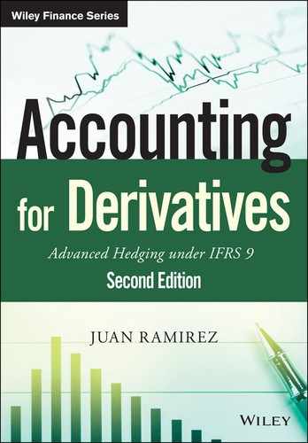
ABC designated the swap as the hedging instrument in a cash flow hedge of the highly expected cash flows stemming from the floating rate bond. The effective amounts of the change in fair value of the swap would be recognised in equity. Following the bond issuance, the amounts accumulated in equity would be subsequently recycled to profit or loss when the bond coupons impacted profit or loss. If the hedge was well constructed, the effective interest rate of the new bond would be close to the sum of the swap fixed rate and the credit spread, or 5.61% (=4.61% + 1%), as shown in Figure 7.4.
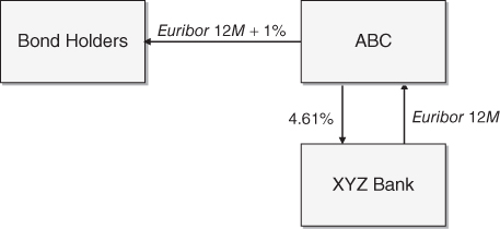
Figure 7.4 Hedging strategy interest flows.
7.10.2 Hedging Relationship Documentation
ABC documented the hedging relationship as follows:
| Hedging relationship documentation | |
| Risk management objective and strategy for undertaking the hedge | The objective of the hedge is to eliminate the variability of the highly expected future cash outflows stemming from a planned issuance of a floating rate bond by the entity. This hedging objective is consistent with the group's overall interest rate risk management strategy of managing the exposure to interest rate risk through the proportion of fixed and floating rate net debt in its total debt portfolio with interest rate swaps, caps and collars. Interest rate risk. The designated risk being hedged is the risk of changes in the EUR value of the hedged item attributable to changes in the Euribor interest rates. Fair value changes attributable to credit or other risks are not hedged in this relationship. Accordingly, the expected 100 basis points credit spread is excluded from the hedging relationship |
| Type of hedge | Cash flow hedge |
| Hedged item | The coupon cash flows of a 3-year floating rate bond highly expected to be issued on 15 July 20X0. The issuance is highly expected to occur as it has been approved by the Board of Directors and a group of banks have been mandated |
| Hedging instrument | The interest rate swap with reference number 014569. The main terms of the swap are a EUR 100 million notional, a forward starting date on 15 July 20X0, a 3-year maturity, a 4.61% fixed rate to be received by the entity and a Euribor 12-month rate to be paid by the entity. The counterparty to the swap is XYZ Bank and the credit risk associated with this counterparty is considered to be very low |
| Hedge effectiveness assessment | See below |
7.10.3 Hedge Effectiveness Assessment
Hedge effectiveness will be assessed by comparing changes in the fair value of the hedging instrument to changes in the fair value of a hypothetical derivative. The terms of the hypothetical derivative are such that its fair value changes exactly offset the changes in fair value of the hedged item for the risk being hedged. The hypothetical derivative is a theoretical interest rate swap with no counterparty credit risk and with zero initial fair value, whose main terms are as follows:
| Hypothetical derivative terms | |
| Trade date | 1 January 20X0 |
| Start date | 15 July 20X0 |
| Counterparties | ABC and credit risk-free counterparty |
| Maturity | 3 years (15 July 20X3) |
| Notional | EUR 100 million |
| ABC pays | Euribor 12M annually, actual/360 basis |
| ABC receives | 4.615% annually, 30/360 basis |
| Euribor fixing | Euribor is fixed 2 days prior to the commencement of the annual interest period |
| Initial fair value | Zero |
The fixed rate of the hypothetical derivative is higher than that of the hedging instrument due to the absence of CVA in the former.
Changes in the fair value of the hedging instrument (i.e., the swap) will be recognised as follows:
- The effective part of the gain or loss on the hedging instrument will be recognised in the cash flow hedge reserve of equity. Following the bond issuance, the amounts accumulated in equity will be reclassified to profit or loss in the same period during which the hedged expected future cash flows affect profit or loss, adjusting interest expense.
- The ineffective part of the gain or loss on the hedging instrument will be recognised in profit or loss, as other financial income/expenses.
Hedge effectiveness will be assessed prospectively at hedging relationship inception, on an ongoing basis at least upon each reporting date and upon occurrence of a significant change in the circumstances affecting the hedge effectiveness requirements.
The hedging relationship will qualify for hedge accounting only if all the following criteria are met:
- The hedging relationship consists only of an eligible hedge item and hedging instrument. The hedge item is eligible as it is a group of highly expected cash flows that will expose the entity to fair value risk, will affect profit or loss and is reliably measurable. The hedging instrument is eligible as it is a derivative that does not result in a net written option.
- At hedge inception there is a formal designation and documentation of the hedging relationship and the entity's risk management objective and strategy for undertaking the hedge.
- The hedging relationship is considered effective.
The hedging relationship will be considered effective if the following three requirements are met:
- There is an economic relationship between the hedged item and the hedging instrument.
- The effect of credit risk does not dominate the value changes that result from that economic relationship.
- The hedge ratio of the hedging relationship is the same as that resulting from the quantity of hedged item that the entity actually hedges and the quantity of the hedging instrument that the entity actually uses to hedge that quantity of hedged item. The hedge ratio should not be intentionally weighted to create ineffectiveness.
Whether there is an economic relationship between the hedged item and the hedging instrument will be assessed on a qualitative basis by comparing the critical terms (notional, interest periods, underlying and fixed rates) of the hypothetical derivative and the hedging instrument. The assessment will be complemented by a quantitative assessment using the scenario analysis method for one scenario in which Euribor interest rates will be shifted upwards by 2% and the changes in fair value of the hypothetical derivative and the hedging instrument compared.
7.10.4 Hedge Effectiveness Assessment Performed at the Start of the Hedging Relationship
On 1 January 20X0 and at each reporting date ABC performed a hedge effectiveness assessment. The documentation related to the assessment performed on 1 January 20X0 was described in Section 7.9.4.
The following potential sources of ineffectiveness were identified:
- a substantial deterioration in credit risk of either the entity or the counterparty to the hedging instrument; and
- a change in the timing or amounts of the hedged highly expected cash flows.
The hedge ratio was set at 1:1.
7.10.5 Fair Valuations, Effective/Ineffective Amounts and Cash Flow Calculations
Suppose that ABC reported its financial statements on an annual basis on 31 December.
Fair Valuations of Hedging Instrument and Hypothetical Derivative
As an example, the following table details the fair valuation of the hedging instrument on 31 December 20X0:
| Euribor | Discount factor | Expected floating leg cash flow | Fixed leg cash flow | Expected settlement amount (1) | Present value (2) | |
| 15-Jul-X1 | 4.30% (3) | 0.9771 | 2,287,000 (4) | <2,476,000> (5) | <189,000> | <185,000> |
| 15-Jul-X2 | 4.70% (6) | 0.9327 | 4,765,000 (7) | <4,610,000> (8) | 155,000 | 145,000 |
| 15-Jul-X3 | 5.12% | 0.8867 | 5,191,000 | <4,610,000> | 581,000 | 515,000 |
| CVA/DVA | <7,000> | |||||
| Total | 468,000 |
Notes:
(1) Expected settlement amount = Expected floating leg cash flow + Fixed leg cash flow
(2) Present value = Expected settlement amount × Discount factor
(3) 4.30% was the Euribor rate, on an actual/360 basis, from 31-Dec-20X0 to 15-Jul-20X1, used to calculate the discount factor
(4) 100 mn × 4.20% × 196/360, where 4.20% was the Euribor 12M fixed on 13-Jul-20X0 and 196 is the number of calendar days from 31-Dec-20X0 to 15-Jul-20X1
(5) 100 mn × 4.61% × 196/365, where 4.61% was the swap's fixed rate and 196 is the number of calendar days from 31-Dec-20X0 to 15-Jul-20X1. Although the fixed rate basis was 30/360, it was approximated with an actual/365 basis to keep it simpler
(6) The expected Euribor 12-month rate, as of 31 December 20X0, to be fixed on 13 July 20X1 (i.e., two business days prior to the commencement of the interest period)
(7) 100 mn × 4.70% × 365 /360, where 4.70% was the expected Euribor 12M to be fixed on 13-Jul-20X1 and 365 is the number of calendar days from 15-Jul-20X1 to 15-Jul-20X2
(8) 100 mn × 4.61%, where 4.61% was the swap's fixed rate
Similarly, the following table details the fair valuation of the hypothetical derivative on 31 March 20X0:
| Date | Euribor 12M | Discount factor | Expected floating leg cash flow | Fixed leg cash flow (*) | Expected settlement amount | Present value |
| 15-Jul-X1 | 4.30% | 0.9771 | 2,287,000 | <2,478,000> | <191,000> | <187,000> |
| 15-Jul-X2 | 4.70% | 0.9327 | 4,765,000 | <4,615,000> | 150,000 | 140,000 |
| 15-Jul-X3 | 5.12% | 0.8867 | 5,191,000 | <4,615,000> | 576,000 | 511,000 |
| CVA/DVA | -0- | |||||
| Total | 464,000 |
(*) Fixed leg cash flow = 100 mn × 4.615%
The fair values of the hedging instrument and the hypothetical derivative at each relevant date were as follows:
| Date | Hedging instrument fair value | Period change | Cumulative change | Hypothetical derivative fair value | Cumulative change | |
| 1-Jan-X0 | -0- | — | — | -0- | — | |
| 31-Dec-X0 | 468,000 | 468,000 | 468,000 | 464,000 | 464,000 | |
| 31-Dec-X1 | 779,000 | 311,000 | 779,000 | 781,000 | 781,000 | |
| 31-Dec-X2 | 264,000 | <515,000> | 264,000 | 264,000 | 264,000 | |
| 15-Jul-X3 | -0- | <264,000> | -0- | -0- | -0- |
Effective and Ineffective Amounts
The ineffective part of the change in fair value of the swap was the excess of its cumulative change in fair value over that of the hypothetical derivative. The effective and ineffective parts of the change in fair value of the swap were the following (see Section 5.5.6 for an explanation of the calculations):
| 31-Dec-X0 | 31-Dec-X1 | 31-Dec-X2 | 15-Jul-X3 | |
| Cumulative change in fair value of hedging instrument | 468,000 | 779,000 | 264,000 | -0- |
| Cumulative change in fair value of hypothetical derivative | 464,000 | 781,000 | 264,000 | -0- |
| Lower amount | 464,000 | 779,000 | 264,000 | -0- |
| Previous cumulative effective amount | — | 464,000 | 775,000 | 264,000 |
| Available amount | 464,000 | 315,000 | <511,000> | <264,000> |
| Period change in fair value of hedging instrument | 468,000 | 311,000 | <515,000> | <264,000> |
| Effective part | 464,000 | 311,000 | <511,000> | <264,000> |
| Ineffective part | 4,000 | Nil | <4,000> | Nil |
Bond and Swap Accrual Amounts
| Euribor 12M (1) | Days (2) | Swap settlement amount accrual (3) | Bond coupon accrual (4) | |
| 31-Dec-X0 | 4.20% | 169 | <163,000> | <2,441,000> |
| 15-Jul-X1 | 4.20% | 196 | <189,000> | <2,831,000> |
| 31-Dec-X1 | 4.70% | 169 | 72,000 | <2,676,000> |
| 15-Jul-X2 | 4.70% | 196 | 83,000 | <3,103,000> |
| 31-Dec-X2 | 5.05% | 169 | 236,000 | <2,840,000> |
| 15-Jul-X3 | 5.05% | 196 | 274,000 | <3,294,000> |
Notes:
(1) Euribor 12-month fixed on the prior 13 July (i.e., 2 days prior to the interest period)
(2) Calendar days from the previous date (i.e., either from the previous 15 July or 31 December, as appropriate)
(3) 100 mn × Euribor 12M × Days/360 − 100 mn × 4.61% × Days/365
(4) 100 mn × (Euribor 12M + 1%) × Days/360
7.10.6 Accounting Entries
Suppose that ABC reported its financial statements on an annual basis on 31 December. The required journal entries were the following.
- Entries on 1 January 20X0
No journal entries were required to record the swap since its fair value was zero at inception.
- Entries on 15 July 20X0
The bond was issued at par.
- Entries on 31 December 20X0
The bond's accrued coupon was EUR 2,441,000.
- The swap's accrued settlement amount was EUR <163,000>.
- The change in fair value of the swap since the last valuation was a EUR 468,000 gain, split between a EUR 464,000 effective amount recorded in the cash flow hedge reserve of OCI and a EUR 4,000 ineffective amount recorded as other financial income in profit or loss.
- Entries on 15 July 20X1
The bond's accrued coupon was EUR 2,831,000. The EUR 5,272,000 coupon was paid.
- The swap's accrued settlement amount was EUR <189,000>. The EUR <352,000> settlement amount was paid.
- Entries on 31 December 20X1
The bond's accrued coupon was EUR 2,676,000. The swap's accrued settlement amount was EUR 72,000. The change in fair value of the swap since the last valuation was a EUR 311,000 gain, fully deemed to be effective and recorded in the cash flow hedge reserve of OCI.
- Entries on 15 July 20X2
The bond's accrued coupon was EUR 3,103,000. The EUR 5,779,000 coupon was paid. The swap's accrued settlement amount was EUR 83,000. The EUR 155,000 settlement amount was received.
- Entries on 31 December 20X2
The bond's accrued coupon was EUR 2,840,000. The swap's accrued settlement amount was EUR 236,000. The change in fair value of the swap since the last valuation was a EUR 515,000 loss, split between a EUR <511,000> effective amount recorded in the cash flow hedge reserve of OCI and a EUR <4,000> ineffective amount recorded as other financial expenses in profit or loss.
- Entries on 15 July 20X3
The bond's accrued coupon was EUR 3,294,000. Both the EUR 6,134,000 coupon and the EUR 100 million principal were paid. The swap's accrued settlement amount was EUR 274,000. The EUR 510,000 settlement amount was received. The change in fair value of the swap since the last valuation was a EUR 264,000 loss, fully deemed to be effective and recorded in the cash flow hedge reserve of OCI.
7.10.7 Concluding Remarks
In order to assess whether ABC achieved its objective of funding itself at 5.61%, let us take a look at ABC's profit or loss statement during the first yearly period (from 15 July 20X0 to 15 July 20X1):
| Profit or Loss Interest Income/Expense From 15-Jul-X0 to 15-Jul-X1 |
|
| Entries on 30-Dec-X0: | |
| Bond coupon accrual | <2,441,000> |
| Swap settlement amount accrual | <163,000> |
| Entries on 15-Jul-X1: | |
| Bond coupon accrual | <2,831,000> |
| Swap settlement accrual | <189,000> |
| Total | <5,624,000> |
The total interest expense for the period was EUR 5,624,000. This expense implied an interest rate of 5.624% on a 30/360 basis. ABC's objective was to fund itself at 5.61% (4.61% swap rate plus 1.00% credit spread), or incurring an overall interest expense of EUR 5,610,000 (=100 mn × 5.61%). Therefore, ABC incurred an interest expense remarkably close to its funding objective. Additionally, ABC's profit or loss during the period recognised other financial income of EUR 4,000 due to hedge ineffectiveness.
7.11 CASE STUDY: HEDGING A FIXED RATE LIABILITY WITH A SWAP IN ARREARS
This case study illustrates the accounting treatment of a hedge of a fixed rate liability with a swap in arrears. This hedging strategy takes advantage of an unusually steep yield curve. The fixed legs of a swap in arrears and a standard swap are identical. The difference between them lies in the fixing of the floating leg:
- In a standard swap, the Euribor rate is set at the beginning of the interest period (specifically, two business days prior to the commencement of the period).
- In a swap in arrears, the Euribor rate is set at the end of the interest period (specifically, two business days prior to the end of the period).
The payment of the floating-leg interest is made at the end of the interest period. For example, suppose that the interest period of the floating leg starts on 15 July 20X0 and ends on 15 July 20X1, and that the underlying variable is the Euribor 12-month rate. Under a standard swap, the Euribor 12-month rate will be fixed on 13 July 20X0 and the floating leg interest will be paid on 15 July 20X1 (see Figure 7.5). Under a swap in arrears, the Euribor 12-month rate will be fixed on 13 July 20X1 and the floating leg interest will be paid on 15 July 20X1 (see Figure 7.5).

Figure 7.5 Floating leg interest period – standard swap versus swap in arrears.
7.11.1 Background Information
On 1 January 20X0, ABC issued at par a fixed rate bond with the following characteristics:
| Bond terms | |
| Issue date | 1 January 20X0 |
| Issuer | ABC |
| Issue proceeds | EUR 100 million (100% of notional) |
| Expected maturity | 3 years (31 December 20X2) |
| Notional | EUR 100 million |
| Coupon | 6.12% annually, 30/360 basis |
ABC's interest rate risk management strategy was to immediately swap to floating all new debt issues and later, as part of its overall hedging policy, decide which fixed-floating mix was appropriate for the whole corporation. First, ABC considered entering into a standard swap in which ABC would pay Euribor 12-month and receive 5.12%. Through the standard swap, ABC would be effectively funding itself at Euribor 12M plus 100 bps (=6.12% – 5.12%). Because the EUR yield curve was unusually steep, ABC preferred instead to enter into a swap in arrears with the following terms:
| Interest rate swap-in-arrears terms | |
| Trade date | 1 January 20X0 |
| Start date | 1 January 20X0 |
| Counterparties | ABC and XYZ Bank |
| Maturity | 3 years (31 December 20X2) |
| Notional | EUR 100 million |
| ABC receives | 5.70% annually, 30/360 basis |
| ABC pays | Euribor 12M annually, actual/360 basis |
| Euribor fixing | Euribor is fixed 2 days prior to the end of the annual interest period |
| Initial fair value | Zero |
Under the swap in arrears, ABC paid annually Euribor 12-month in arrears and received annually 5.70%. ABC then used the 5.70% received and added 0.42% to pay the 6.12% bond interest. The combination of the bond and the swap resulted in ABC paying an interest of Euribor 12M in arrears plus 42 bps, as shown in Figure 7.6. The 42 bps spread was the difference between the bond coupon (6.12%) and the swap fixed rate (5.70%).
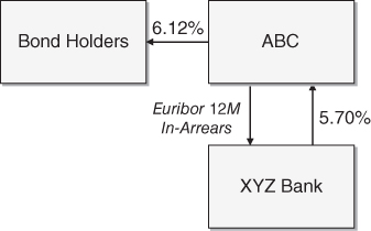
Figure 7.6 Hedging strategy interest flows.
The swap in arrears was designated as the hedging instrument in a fair value hedge of the bond.
7.11.2 Hedging Relationship Documentation
ABC documented the hedging relationship as follows:
| Hedging relationship documentation | |
| Risk management objective and strategy for undertaking the hedge | The objective of the hedge is to reduce the variability of the fair value of a fixed rate bond issued by the entity. This hedging objective is consistent with the group's overall interest rate risk management strategy of transforming all new issued debt into floating rate, and thereafter managing the exposure to interest rate risk through the proportion of fixed and floating rate net debt in its total debt portfolio. Interest rate risk. The designated risk being hedged is the risk of changes in the EUR fair value of the hedged item attributable to changes in the Euribor interest rate. Fair value changes attributable to credit or other risks are not hedged in this relationship. Accordingly, the 60 basis points credit spread is excluded from the hedging relationship |
| Type of hedge | Fair value hedge |
| Hedged item | The coupons and principal of the 3-year 6.12% fixed rate bond with reference number 678908. As the bond credit spread (100 basis points) is excluded from the hedging relationship, only the cash flows related to the interest rate component of the coupons will be part of the hedging relationship (i.e., those corresponding to a 5.12% rate or EUR 5.12 million). The EUR 100 million principal is included in the hedging relationship in its entirety |
| Hedging instrument | The interest rate swap in arrears with reference number 014573. The main terms of the swap are a EUR 100 million notional, a 3-year maturity, a 5.70% fixed rate to be received by the entity and a Euribor 12-month rate to be paid by the entity. The Euribor 12-month rate is fixed two business days prior to the end of the interest period. The counterparty to the swap is XYZ Bank and the credit risk associated with this counterparty is considered to be very low |
| Hedge effectiveness assessment | See next below |
7.11.3 Hedge Effectiveness Assessment
Hedge effectiveness will be assessed by comparing changes in the fair value of the hedging instrument to changes in the fair value of the hedged item. Changes in the fair value of the hedging instrument (i.e., the swap) will be recognised as follows:
- The effective part of the gain or loss on the hedging instrument will be recognised in profit or loss, adjusting interest income/expense.
- The ineffective part of the gain or loss on the hedging instrument will be recognised in profit or loss, as other financial income/expenses.
Hedge effectiveness will be assessed prospectively at hedging relationship inception, on an ongoing basis at least upon each reporting date and upon occurrence of a significant change in the circumstances affecting the hedge effectiveness requirements.
The hedging relationship will qualify for hedge accounting only if all the following criteria are met:
- The hedging relationship consists only of eligible hedge items and hedging instruments. The hedge item is eligible as it is an already recognised liability that exposes the entity to fair value risk, affects profit or loss and is reliably measurable. The hedging instrument is eligible as it is a derivative that does not result in a net written option.
- At hedge inception there is a formal designation and documentation of the hedging relationship and the entity's risk management objective and strategy for undertaking the hedge.
- The hedging relationship is considered effective.
The hedging relationship will be considered effective if the following three requirements are met:
- There is an economic relationship between the hedged item and the hedging instrument,
- The effect of credit risk does not dominate the value changes that result from that economic relationship,
- The hedge ratio of the hedging relationship is the same as that resulting from the quantity of hedged item that the entity actually hedges and the quantity of the hedging instrument that the entity actually uses to hedge that quantity of hedged item. The hedge ratio should not be intentionally weighted to create ineffectiveness.
Whether there is an economic relationship between the hedged item and the hedging instrument will be assessed on a quantitative basis using the regression analysis method, comparing the changes in fair value of the hedged item and the hedging instrument.
7.11.4 Hedge Effectiveness Assessment Performed at the Start of the Hedging Relationship
On 1 January 20X0 ABC performed a hedge effectiveness assessment which was documented as described next.
The hedging relationship was considered effective as the following three requirements were met:
- There was an economic relationship between the hedged item and the hedging instrument.
- The effect of credit risk did not dominate the value changes resulting from that economic relationship as the credit ratings of both the entity and XYZ Bank were considered sufficiently strong.
- The hedge ratio of the hedging relationship was the same as that resulting from the quantity of hedged item that the entity actually hedged and the quantity of the hedging instrument that the entity actually used to hedge that quantity of hedged item. The hedge ratio was not intentionally weighted to create ineffectiveness.
A quantitative assessment was performed to support the conclusion that the hedging instrument and the hedged item had values that would generally move in opposite directions. The quantitative assessment consisted of a regression analysis performed as shown in Figure 7.7.
Figure 7.7 Swap in arrears – regression analysis.
A regression analysis assesses the level of correlation between changes in the clean (i.e., excluding accruals) fair value of the hedging instrument and the changes in the clean fair value of the hedged item, using historical interest rate information. If a high correlation exists, then movements in the fair value of the bond can be reasonably expected to trigger similar offsetting movements in the fair value of the swap. The analysis was based on historical EUR interest rates over the previous 15 years (the “historical time horizon”). The historical time horizon was divided into 156 “simulation periods” of 3 years each, as shown in Figure 7.8.

Figure 7.8 Regression analysis – simulation periods.
Each simulation period had an inception date and three subsequent annual balance sheet dates. During each simulation period, the behaviour of an equivalent hedging relationship using the historical data was simulated. At the beginning of the simulation period, the terms of the hedging instrument and hedged item were determined as if the hedge were entered into on that date. The terms were such that the simulated hedge terms were equivalent to the actual terms but taking into account the market rates prevailing at the beginning of the simulation period. Each observation pair (X, Y) was generated by computing the cumulative change in the fair value of the simulation hedging instrument (variable X) and the cumulative change in fair value of the simulation hypothetical derivative (observation Y). Figure 7.9 highlights the process for the first simulation, which started 15 years prior to 1 January 20X0.
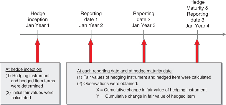
Figure 7.9 Regression analysis – simulation periods.
The results of the regression analysis showed an R-squared of 90.2%, a slope of the regression line of 1.00, and the F-statistic indicated statistical significance at the 95% confidence level. Based on these results, the entity concluded that the change in fair value of the hedged item was expected to be substantially offset by the change in fair value of the hedging instrument, corroborating that both elements had values that would generally move in opposite directions.
The following potential sources of ineffectiveness were identified:
- a substantial deterioration in credit risk of either the entity or the counterparty to the hedging instrument; and
- a change in the timing or amounts of the hedged highly expected cash flows.
The hedge ratio was set at 1:1.
ABC also performed assessments at each reporting date, yielding similar conclusions. These assessments have been omitted to avoid unnecessary repetition. The credit risk of the entity and the counterparty to the hedging instrument were continuously monitored and throughout the hedge life both credit risks were considered to be very low.
7.11.5 Fair Valuations, Effective/Ineffective Amounts and Cash Flow Calculations
Fair Valuations of the Hedging Instrument
The Euribor 12-month rate fixings at the relevant dates were as follows:
| Euribor 12M fixings | |
| 29-Dec-W9 | 4.44% |
| 29-Dec-X0 | 4.94% |
| 29-Dec-X1 | 5.64% |
| 29-Dec-X2 | 6.00% |
The fair value of the swap was computed by summing the present value of each expected future net settlement, and adjusting for CVA/DVA. The fair value of the swap on 1 January 20X0 was zero.
The fair value of the swap on 31 December 20X0 was calculated using the market yield curve on that date as follows:
| Cash flow date | Discount factor | Expected Euribor 12M | Expected floating leg cash flow | Fixed leg cash flow | Net amount | Present value |
| 31-Dec-X1 | 0.9523 | 5.70% | <5,779,000> (1) | 5,700,000 (2) | <79,000> (3) | <75,000> (4) |
| 31-Dec-X2 | 0.9003 | 6.10% | <6,185,000> | 5,700,000 | <485,000> | <437,000> |
| CVA/DVA | 8,000 | |||||
| Fair value | <504,000> |
Notes:
(1) 100 mn × 5.70% × 365/360, where 5.70% was the expected Euribor 12M rate to be fixed on 29-Dec-X1 (i.e., two business days prior to the end date of the interest period) and 365 is the number of calendar days from 31-Dec-X0 to 31-Dec-X1)
(2) 100 mn × 5.70%, where 5.70% was the swap fixed rate
(3) <5,779,000> + 5,700,000
(4) <79,000> × 0.9523
The fair value of the swap on 31 December 20X1 was calculated using the market yield curve on that date as follows:
| Date | Discount factor | Expected Euribor 12M | Expected floating leg cash flow | Fixed leg cash flow | Net amount | Present value |
| 31-Dec-X2 | 0.9459 | 6.14% | <6,225,000> (1) | 5,700,000 (2) | <525,000> (3) | <497,000> (4) |
| CVA/DVA | 5,000 | |||||
| Fair value | <492,000> |
Notes:
(1) 100 mn × 6.14% × 365/360, where 6.14% was the expected Euribor 12-month rate to be fixed on 29-Dec-X2 (i.e., two business days prior to the end date of the interest period) and 365 is the number of calendar days from 31-Dec-X1 to 31-Dec-X2)
(2) 100 mn × 5.70%, where 5.70% was the swap fixed rate
(3) <6,225,000> + 5,700,000
(4) <525,000> × 0.9459
The fair value of the swap on 31 December 20X2 was zero.
Fair Valuations of the Hedged Item
The fair value of the hedged item was computed by summing up the present value of each future EUR 5.12 million fixed cash flow. Remember that the risk being hedged was interest rate risk only. Therefore, changes in the fair value of the bond due to changes in ABC's credit spread were not part of the hedged item fair valuations. The cash flows being hedged were the first EUR 5,120,000 of each annual coupon, a portion of the EUR 6,120,000 annual coupon.
The fair value of the hedged item on 1 January 20X0 was EUR <100 million>.
The fair value of the bond on 31 December 20X0 was calculated using the market yield curve on that date as follows:
| Date | Discount factor | Expected cash flow | Present value |
| 31-Dec-X1 | 0.9523 | <5,120,000> (1) | <4,876,000> |
| 31-Dec-X3 | 0.9003 | <105,120,000> | <94,640,000> |
| Fair value | <99,516,000> |
Notes:
(1) The hedged cash flow of the bond coupon
(2) 5,120,000 × 0.9523
The fair value of the bond on 31 December 20X1 was calculated using the market yield curve on that date as follows:
| Date | Discount factor | Expected cash flow | Present value |
| 31-Jul-X3 | 0.9459 | <105,120,000> | <99,433,000> |
| Fair value | <99,433,000> |
The fair value of the bond on 31 December 20X2 was EUR <100 million>.
Calculations of Effective and Ineffective Amounts
The period changes in fair value of the hedging instrument and the hedged item were as follows:
| Date | Hedging instrument fair value | Period change | Hedged item fair value | Period change | |
| 31-Jul-X0 | -0- | — | <100,000,000> | — | |
| 31-Dec-X0 | <504,000> | <504,000> | <99,516,000> | 484,000 | |
| 31-Dec-X1 | <492,000> | 12,000 | <99,433,000> | 83,000 | |
| 31-Dec-X2 | -0- | 492,000 | <100,000,000> | <567,000> |
The ineffective part of the change in fair value of the hedging instrument was the excess of its period change in fair value over that of the hedged item. The effective and ineffective parts of the period change in fair value of the swap were as follows:
| 31-Dec-X0 | 31-Dec-X1 | 31-Dec-X2 | |
| Period change in fair value of hedging instrument | <504,000> | 12,000 | 492,000 |
| Period change in fair value of hedged item (opposite sign) | <484,000> | <83,000> | 567,000 |
| Lower amount | <484,000> | -0- (*) | 492,000 |
| Effective part | <484,000> | -0- | 492,000 |
| Ineffective part | <20,000> | 12,000 | -0- |
(*) There was no offset between the period change in fair values of the hedging instrument and the hedged item
The effective part of the change in fair value of the hedged item was the effective part of the change in fair value of the hedging instrument (see previous table). Any remainder was considered to be ineffective. The effective and ineffective parts of the period change in fair value of the hedged item were as follows:
| 31-Dec-X0 | 31-Dec-X1 | 31-Dec-X2 | |
| Period change in fair value of hedged item | 484,000 | 83,000 | <567,000> |
| Effective part of change in fair value of hedging instrument (opposite sign) | 484,000 | -0- | <492,000> |
| Ineffective part (excess) | -0- | 83,000 | <75,000> |
Calculations of Bond Coupon and Swap Settlement Amounts
| Cash flow date | Bond coupon | Euribor fixing (in arrears) | Swap settlement amount |
| 31-Dec-X0 | <6,120,000> (1) | 4.94% | 691,000 (2) |
| 31-Dec-X1 | <6,120,000> | 5.64% | <18,000> |
| 31-Dec-X2 | <6,120,000> | 6.00% | <383,000> |
Notes:
(1) 100 mn × 6.12%
(2) 100 mn × 5.70% − 100 mn × 4.94% × 365/360, where 5.70% was the swap's fixed rate, 4.94% was the Euribor 12M rate fixed two business days prior to 31-Dec-X0 (i.e., 29-Dec-X0) and 365 is the number of calendar days from 1-Jan-X0 to 31-Dec-X0)
7.11.6 Accounting Entries
Suppose that ABC reported its financial statements on an annual basis on 31 December. The required journal entries were the following.
- Entries on 1 January 20X0
The bond was issued at par.
- No journal entries were required to record the swap in arrears since its fair value was zero at inception.
- Entries on 31 December 20X0
The EUR 6,120,000 (=100 million × 6.12%) bond coupon was paid.
- The EUR 691,000 swap settlement amount was received.
- The change in fair value of the swap since the last valuation was a EUR 504,000 loss, of which EUR <484,000> was deemed to be effective and recorded as interest expense in profit or loss, while EUR <20,000> was deemed to be ineffective and recorded as other financial expenses in profit or loss.
- The change in fair value of the hedged item since the last valuation was a EUR 484,000 gain, fully deemed to be effective and recorded as interest income in profit or loss.
- Entries on 31 December 20X1
The EUR 6,120,000 (=100 million × 6.12%) bond coupon was paid. The EUR <18,000> swap settlement amount was paid. The change in fair value of the swap since the last valuation was a EUR 12,000 gain, fully deemed to be ineffective and recorded as other financial income in profit or loss. The change in fair value of the hedged item since the last valuation was a EUR 83,000 gain, fully deemed to be ineffective and recorded as other financial income in profit or loss.
- Entries on 31 December 20X2
The EUR 6,120,000 (=100 million × 6.12%) bond coupon was paid. The bond's EUR 100 million principal was repaid. The EUR <383,000> swap settlement amount was paid. The change in fair value of the swap since the last valuation was a EUR 492,000 gain, fully deemed to be effective and recorded as interest income in profit or loss. The change in fair value of the hedged item since the last valuation was a EUR 567,000 loss of which EUR <492,000> was deemed to be effective and recorded as interest expense in profit or loss, while EUR <75,000> was deemed to be ineffective and recorded as other financial expenses in profit or loss.
The following table gives a summary of the accounting entries:
| Cash | Derivative contract | Financial debt | Profit or loss | |
| 1-Jan-20X0 | ||||
| Bond issuance | 100,000,000 | 100,000,000 | ||
| Derivative trade | — | |||
| 31 Dec-20X0 | ||||
| Bond coupon | <6,120,000> | <6,120,000> | ||
| Swap settlement amount | 691,000 | 691,000 | ||
| Swap fair valuation | <504,000> | <504,000> | ||
| Hedged item fair valuation | <484,000> | 484,000 | ||
| 31-Dec-20X1 | ||||
| Bond coupon | <6,120,000> | <6,120,000> | ||
| Swap settlement amount | <18,000> | <18,000> | ||
| Swap fair valuation | 12,000 | 12,000 | ||
| Hedged item fair valuation | <83,000> | 83,000 | ||
| 31-Dec-20X2 | ||||
| Bond coupon | <6,120,000> | <6,120,000> | ||
| Bond principal | <100,000,000> | <100,000,000> | ||
| Swap settlement amount | <383,000> | <383,000> | ||
| Swap fair valuation | 492,000 | 492,000 | ||
| Hedged item fair valuation | 567,000 | <567,000> | ||
| TOTAL | <18,070,000> | -0- | -0- | <18,070,000> |
Note: Total figures may not match the sum of their corresponding components due to rounding.
7.11.7 Concluding Remarks
ABC tried to synthetically convert the 6.12% bond coupon into a floating interest rate. Rather than targeting the cost of funding of Euribor 12-month plus 100 basis points with a standard swap, ABC tried to achieve a slightly better cost of funding by entering into a swap in arrears. The table below summarises the annual cost of funding achieved (“actual funding”) and how it compared to a Euribor 12-month plus 1% funding (“target funding”). By implementing the in-arrears strategy, ABC saved EUR 201,000 in financial costs. Therefore, ABC's view that the interest rate curve on 1 January 20X0 was too steep (i.e., was discounting too high future Euribor 12-month rates) was right.
| Euribor 12M (1) | Target funding (2) | Actual funding | Savings | |
| Period from 1-Jan-X0 to 31-Dec-X0 | 4.44% | <5,516,000> | <5,449,000> | 67,000 |
| Period from 31-Dec-X0 to 31-Dec-X1 | 4.94% | <6,023,000> | <6,043,000> | <20,000> |
| Period from 31-Dec-X0 to 31-Dec-X1 | 5.64% | <6,732,000> | <6,578,000> | 154,000 |
| Total | 201,000 |
Notes:
(1) Euribor 12-month fixed 2 days prior to the commencement of the interest period
(2) 100 mn × (Euribor 12M + 1%) × 365/360
From an accounting perspective, there is a risk of substantial ineffectiveness during the last few reporting dates prior to the end of the hedging relationship.
7.12 CASE STUDY: HEDGING A FLOATING RATE LIABILITY WITH A KIKO COLLAR
This case study illustrates the accounting treatment of a hedge of a floating rate liability with a European KIKO collar. Section 5.13 covered the hedge of a highly expected foreign sale with an FX KIKO forward in which the barriers were continuously observed (an “American” KIKO). The KIKO covered in this section is a “European” KIKO because the barriers were only observed at expiry of the options. Therefore, it was irrelevant whether a barrier was crossed prior to option expiry. In other words, ABC only had to worry about whether the barrier was crossed at expiry. The hedged liability is the same as in Sections 7.5 and 7.6.
This case study also covers a collar whose initial intrinsic and time values were other than zero, showing the substantial operational complexity of having to calculate effective and ineffective amounts, and amounts recognised in the time value reserve, for each separate caplet/floorlet.
7.12.1 Background Information
On 31 December 20X0, ABC issued at par a floating rate bond with the following characteristics:
| Bond terms | |
| Issue date | 31 December 20X0 |
| Maturity | 5 years (31 December 20X5) |
| Notional | EUR 100 million |
| Coupon | Euribor 12M + 1.50% annually, actual/360 basis |
| Euribor fixing | Euribor is fixed at the beginning of the annual interest period |
ABC had the view that the curve was too steep and that the Euribor 12-month rate was unlikely, during the next 5 years, either to rise above 5.25% or fall below 2.90%. To incorporate this view, ABC hedged its exposure under the bond to Euribor 12-month rate increases by entering into a European KIKO collar. The KIKO collar comprised a knock-out cap and a knock-in floor. The terms of the knock-out cap were as follows:
| Knock-out cap terms | |
| Start date | 31 December 20X0 |
| Counterparties | ABC and XYZ Bank |
| Cap buyer | ABC |
| Maturity | 5 years (31 December 20X5) |
| Notional amount | EUR 100 million |
| Premium | EUR 890,000 |
| Strike | 3.75% annually, actual/360 basis |
| Underlying | Euribor 12-month rate. Euribor is fixed at the beginning of the annual interest period |
| Barrier | 5.25% |
| Knock-out event | Caplet ceases to exist if the Euribor 12-month rate is set at or above the barrier for the interest period ending on the expiry date |
Each caplet could only be exercised if the Euribor 12-month rate was set below 5.25% for the interest period ending on the expiry date. Thus, if at the beginning of an interest period the Euribor 12-month was at or above 5.25%, ABC had no protection for that period. Nonetheless, the remaining caplets remained active. Figure 7.10 depicts the payoff of each caplet.

Figure 7.10 Knock-out caplet payoff (excluding premium).
The main terms of the knock-in floor were as follows:
| Knock-in floor terms | |
| Start date | 31 December 20X0 |
| Counterparties | ABC and XYZ Bank |
| Floor buyer | XYZ Bank |
| Maturity | 5 years (31 December 20X5) |
| Notional amount | EUR 100 million |
| Premium | EUR 890,000 |
| Strike | 3.52% annually, actual/360 basis |
| Underlying | Euribor 12-month rate Euribor is fixed at the beginning of the annual interest period |
| Barrier | 2.90% |
| Knock-in event | Floorlet can only be exercised if the Euribor 12-month rate is set at or below the barrier for the interest period ending on the expiry date |
Each floorlet could only be exercised if the Euribor 12-month rate was set at or below 2.90% for the interest period ending on the expiry date. In other words, if at the beginning of an interest period Euribor 12-month was above 2.90%, the corresponding floorlet would not be exercised and, consequently, ABC would not need to make any payment under the floorlet. Nonetheless, any remaining floorlets could be activated at their corresponding expiry, were the Euribor 12-month rate at the commencement of their interest period to be below 2.90%. Figure 7.11 depicts the payoff of each floorlet.
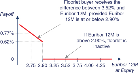
Figure 7.11 Knock-in floorlet payoff (excluding premium).
There were four scenarios depending on the behaviour of the Euribor 12-month rate at each expiry date.
| 2.90% barrier | 5.25% barrier | Equivalent position | Comments |
| Not hit | Not hit | Purchased 3.75% cap | Best scenario. ABC had protection and participated in Euribor 12M rate declines |
| Hit | Not hit | 3.75%–3.52% collar | Good scenario, ABC ended up with a collar at much better terms than a market swap (swap would have been 3.86%) |
| Not Hit | Hit | No derivative | Bad scenario, ABC ended up having no hedge in place |
| Hit | Hit | Sold 2.90% floor | Worst scenario, ABC lost its protection and could not benefit from declining Euribor 12M rates below 3.52% |
7.12.2 Split between Hedge Accounting Compliant Derivative and Residual Derivative
From an accounting perspective, IFRS 9 does not provide particular guidance about the application of hedge accounting for exotic hedging strategies such as the KIKO collar. Even if an entity applies hedge accounting, a decision that an auditor may well challenge, substantial ineffectiveness may arise. Nonetheless, IFRS 9 provides a relatively clear guidance on hedging strategies involving swaps, caps and collars. From an accounting perspective, a sound strategy would be to contractually split the KIKO collar into two parts, a first part eligible for hedge accounting and a second part treated as undesignated, reducing the potential impact on profit or loss volatility. ABC considered the following choices:
- Divide the KIKO into two contracts: (i) a standard collar and (ii) a “residual” derivative. The standard collar would be the combination of a bought 3.75% cap and a sold 2.90% floor. The residual derivative would be the rest of the KIKO collar payoff not included in the standard collar.
- Divide the KIKO into two contracts: (i) a standard collar and (ii) a “residual” derivative. The standard collar would be the combination of a bought 3.75% cap and a sold 3.52% floor. The residual derivative would be the rest of the KIKO collar payoff not included in the standard collar.
- Divide the KIKO into two contracts: (i) a combination of two standard collars, and (ii) a “residual” derivative. One standard collar would be the combination of a bought 3.75% cap and a sold 2.90% floor. The other standard collar would be a bought very out-of-the money floor (e.g., with a 0.50% floor rate) and a sold 5.25% cap. The residual derivative would be the rest of the KIKO collar payoff not included in the combination of standard collars. This alternative was valid under IFRS 9 as the sold floors were entered into in combination with purchased caps and the combination did not result in a net premium to be received by the entity. ABC discarded this choice as it was too complex.
- Consider the KIKO in its entirety as eligible for hedge accounting, if the corresponding requirements were met. Under this approach, ABC would designate the KIKO collar in its entirety as the hedging instrument in a hedging relationship. This approach would have been, in my view, quite challenging to apply. Effectiveness would be assessed comparing the changes in the fair value of the KIKO forward against those of a hypothetical derivative – a swap with an initial zero fair value and no counterparty credit risk. Due to their very different payoffs, the economic relationship requirement is likely not to be met for scenarios in which Euribor 12-month reaches 5.25% (when the protection is lost). As a result, ABC discarded this choice.
- Consider the whole KIKO as undesignated. Whilst this was the simplest choice, ABC discarded this choice due to its potential adverse impact on profit or loss volatility.
ABC was thus left with only the first two choices. The first choice was better if Euribor 12-month rates traded well above 2.90%. Otherwise the second choice was preferable. Because it expected the Euribor 12-month to trade, during the next 5 years, well above 2.90%, ABC selected the first choice:
- The standard collar combined a purchased 3.75% cap and a sold 2.90% floor (see Figure 7.12). The effective changes in the intrinsic value of the collar would be recorded in equity (in the cash flow hedge reserve) and subsequently reclassified to profit or loss when the hedged cash flows impacted profit or loss. Changes in the time value of the collar would be recorded in equity to the extent that they related to the hedged item.
- The residual derivative would have terms such that when combined with the standard collar terms, the KIKO collar terms were obtained. Changes in fair value of the residual derivative would be recorded in profit or loss as it was classified as undesignated.
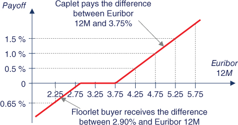
Figure 7.12 Hedging instrument payoff (bought 3.75% cap, sold 2.90% floor).
Remember that the two parts had to be formalised in separate contracts. The main terms of the standard collar were as follows:
| Standard collar terms | ||||
| Cap terms | Floor terms | |||
| Start date | 31 December 20X0 | Start date | 31 December 20X0 | |
| Counterparties | ABC and XYZ Bank | Counterparties | ABC and XYZ Bank | |
| Cap buyer | ABC | Floor seller | ABC | |
| Maturity | 5 years (31- Dec-X5) | Maturity | 5 years (31-Dec-X5) | |
| Notional amount | EUR 100 million | Notional amount | EUR 100 million | |
| Premium | EUR 2,237,000 | Premium | EUR 280,000 | |
| Strike | 3.75% annually, actual/360 basis | Strike | 2.90% annually, actual/360 basis | |
| Underlying | Euribor 12M rate set at the beginning of the interest period ending on the expiry date | Underlying | Euribor 12M rate set at the beginning of the interest period ending on the expiry date | |
The residual derivative comprised the following two options:
- a sold knock-in cap with a 3.75% strike and a 5.25% barrier; and
- a sold digital floor with strike 2.90% and 0.62% payoff (=3.52% – 2.90%).
7.12.3 Hedging Relationship Documentation
ABC documented the hedging relationship as follows:
| Hedging relationship documentation | |
| Risk management objective and strategy for undertaking the hedge | The objective of the hedge is to protect the variability of the cash flows stemming from the floating rate coupon payments related to a debt instrument issued by the entity against unfavourable movements in the Euribor 12-month rate above 3.75%. To achieve this objective and to reduce the hedge overall cost, the entity does not benefit from favourable movements in the Euribor 12M below 2.90%. This hedging objective is consistent with ABC's overall risk management strategy of managing the exposure to interest rate risk through the proportion of fixed and floating rate net debt in its total debt portfolio, using swaps and interest rate options. Interest rate risk. The designated risk being hedged is the risk of changes in the EUR value of the hedged cash flows due to movements in the Euribor 12-month interest rate |
| Type of hedge | Cash flow hedge |
| Hedged item | The cash flows stemming from the coupons of the bond with reference number 08759 issued on 31 December 20X0 with a 5-year maturity, a EUR 100 million notional, and a Euribor 12-month plus 1.50% annual coupon. The coupons are highly expected to occur as the bond has already been issued. The 1.50% credit spread is excluded from the hedging relationship |
| Hedging instrument | The intrinsic value of a collar (the combination of a purchased cap and a sold floor) with reference number 014577. The main terms of the collar are a EUR 100 million notional, a 5-year maturity, a 3.75% cap rate, a 2.90% floor rate, a Euribor 12-month interest rate underlying and a EUR 1,957,000 up-front cost. The counterparty to the collar is XYZ Bank and the credit risk associated with this counterparty is considered to be very low. For the avoidance of doubt, the collar's time value is excluded from the hedging relationship |
| Hedge effectiveness assessment | See below |
7.12.4 Hedge Effectiveness Assessment
Hedge effectiveness will be assessed by comparing changes in the fair value of the hedging instrument to changes in the fair value of a hypothetical derivative. Effectiveness will be assessed only during those periods in which there is a change in intrinsic value.
The next two paragraphs were not included in the hedge documentation, having been added to explain how I selected the terms of the hypothetical derivative.
The hypothetical derivative is a derivative whose changes in fair value perfectly offset the changes in fair value of the hedged item for variations in the risk being hedged. In the case of “one-sided risks” IFRS states that “the hypothetical derivative would represent the intrinsic value of a hypothetical option that at the time of designation of the hedging relationship is at the money if the hedged price level is the current market level, or out of the money if the hedged price level is above (or, for a hedge of a long position, below) the current market level”. IFRS 9 does not provide particular guidance on how the terms of the hypothetical derivative are determined when a combination of options is used. At the time of writing, the accounting community has not reached a consensus on how to set the level of the hypothetical derivative, especially regarding the level of the sold option.
As the risk being hedged was the cash flow exposure to adverse movements in the Euribor 12-month rate above 3.75% while not benefiting from favourable movements in the Euribor 12-month rate below 2.90%, the preliminary levels of the hypothetical derivative were a theoretical interest rate collar with no counterparty credit risk, a 3.75% cap rate and a 2.90% floor rate. The 3.75% cap rate was in-the-money at the start of the hedging relationship because the swap rate was 3.86% (see the case study in Section 7.5). Because the strike rate in a hypothetical derivative has to be either at-the-money or out-of-the-money, the lowest eligible cap rate in our case was 3.86%, the at-the-money level. The floor rate (2.90%) was lower than the swap rate, therefore being out-of-the-money, an eligible level for the hypothetical derivative.
The main terms of the hypothetical derivative were the following:
| Hypothetical derivative terms | ||||
| Cap terms | Floor terms | |||
| Start date | 31 December 20X0 | Trade date | 31 December 20X0 | |
| Buyer | ABC | Buyer | Credit risk-free counterparty | |
| Seller | Credit risk-free counterparty | Seller | ABC | |
| Notional | EUR 100 million | Notional | EUR 100 million | |
| Maturity | 5 years (31 December 20X5) | Maturity | 5 years (31 December 20X5) | |
| Cap rate | 3.86%, actual/360 basis | Floor rate | 2.90%, actual/360 basis | |
| Underlying | Euribor 12-month, fixed at the beginning of the annual interest period ending on the expiry date | Underlying | Euribor 12-month, fixed at the beginning of the annual interest period ending on the expiry date | |
Changes in the fair value of the hedging instrument (i.e., the collar's intrinsic value) will be recognised as follows:
- The effective part of the gain or loss on the hedging instrument will be recognised in the cash flow hedge reserve of OCI in equity. The accumulated amount in equity will be reclassified to profit or loss in the same period during which the hedged expected future cash flow affects profit or loss, adjusting interest expense.
- The ineffective part of the gain or loss on the hedging instrument will be recognised immediately in profit or loss.
The change in time value of the collar (the “actual time value”) will be excluded from the hedging relationship. The changes in actual time value will be recognised temporarily in the time value reserve of equity to the extent that they relate to the hedged item.
Hedge effectiveness will be assessed prospectively at hedging relationship inception, on an ongoing basis at least upon each reporting date and upon occurrence of a significant change in the circumstances affecting the hedge effectiveness requirements.
The hedging relationship will qualify for hedge accounting only if all the following criteria are met:
- The hedging relationship consists only of eligible hedge items and hedging instruments. The hedge item is eligible as it is a group of highly expected forecast cash flows that exposes the entity to fair value risk, affects profit or loss and is reliably measurable. The hedging instrument is eligible as it is a string of derivative combinations that does not result in a net written option and the sold options are designated as an offset to the purchased options.
- At hedge inception there is a formal designation and documentation of the hedging relationship and the entity's risk management objective and strategy for undertaking the hedge.
- The hedging relationship is considered effective.
The hedging relationship will be considered effective if the following three requirements are met:
- There is an economic relationship between the hedged item and the hedging instrument.
- The effect of credit risk does not dominate the value changes that result from that economic relationship.
- The hedge ratio of the hedging relationship is the same as that resulting from the quantity of hedged item that the entity actually hedges and the quantity of the hedging instrument that the entity actually uses to hedge that quantity of hedged item. The hedge ratio should not be intentionally weighted to create ineffectiveness.
Whether there is an economic relationship between the hedged item and the hedging instrument will be assessed on a quantitative basis using the scenario analysis method for two scenarios in which Euribor interest rates will be shifted upwards and downwards by 2% and the changes in fair value of the hypothetical derivative and the hedging instrument compared.
7.12.5 Hedge Effectiveness Assessment Performed at the Start of the Hedging Relationship
The hedging relationship was considered effective as the following three requirements were met:
- There was an economic relationship between the hedged item and the hedging instrument. Based on the quantitative assessment performed, the entity concluded that the change in fair value of the hedged item was expected to be substantially offset by the change in fair value of the hedging instrument, corroborating that both elements had values that would generally move in opposite directions.
- The effect of credit risk did not dominate the value changes resulting from that economic relationship as the credit ratings of both the entity and XYZ Bank were considered sufficiently strong.
- The hedge ratio of the hedging relationship was the same as that resulting from the quantity of hedged item that the entity actually hedged and the quantity of the hedging instrument that the entity actually used to hedge that quantity of hedged item. The hedge ratio was not intentionally weighted to create ineffectiveness.
A quantitative assessment was performed to support the conclusion that the hedging instrument and the hedged item had values that would generally move in opposite directions. The quantitative assessment consisted of two scenario analyses performed as follows:
A parallel shift of +2% occurring on the assessment date was simulated. The fair values of the hedging instrument and the hypothetical derivatives were calculated and compared to their initial fair values. As shown in the table below, the assessment resulted in a high degree of offset, corroborating that both elements had values that would generally move in opposite directions.
| Scenario 1 analysis assessment | ||
| Hedging instrument | Hypothetical derivative | |
| Initial fair value | 1,410,000 (1) | 1,136,000 |
| Final fair value | 9,308,000 | 8,957,000 |
| Cumulative fair value change | 7,898,000 | 7,821,000 |
| Degree of offset | 101.0% (2) | |
Notes:
(1) Only the intrinsic value of the collar was part of the hedging relationship
(2) The degree of offset was not 100% due to the differing cap rates and CVAs/DVAs
Similarly, a parallel shift of –2% occurring on the assessment date was also simulated. As shown in the table below, the assessment resulted in a high degree of offset, corroborating that both elements had values that would generally move in opposite directions.
| Scenario 2 analysis assessment | ||
| Hedging instrument | Hypothetical derivative | |
| Initial fair value | 1,410,000 | 1,136,000 |
| Final fair value | <4,886,000> | <4,985,000> |
| Cumulative fair value change | <6,296,000> | <6,121,000> |
| Degree of offset | 102.9% | |
The following potential sources of ineffectiveness were identified:
- a substantial deterioration in credit risk of either the entity or the counterparty to the hedging instrument; and
- a change in the timing or amounts of the hedged highly expected cash flows.
The hedge ratio was set at 1:1.
ABC also performed assessments on each reporting date, yielding the same conclusions. These assessments have been omitted to avoid unnecessary repetition.
7.12.6 Fair Valuations, Effective/Ineffective Amounts and Cash Flow Calculations
Fair Valuations of the Collar and Residual Derivative
The following table summarises the split between the collar's intrinsic and time values, and the fair value of the residual derivative at each reporting date:
| Date | Collar intrinsic value | Collar time value | Collar total fair value | Residual derivative fair value | KIKO collar fair value (*) |
| 31-Dec-20X0 | 1,410,000 | 547,000 | 1,957,000 | <1,957,000> | 0 |
| 31-Dec-20X1 | 3,618,000 | 297,000 | 3,915,000 | <2,775,000> | 1,140,000 |
| 31-Dec-20X2 | 1,120,000 | 187,000 | 1,307,000 | <974,000> | 333,000 |
| 31-Dec-20X3 | 646,000 | 105,000 | 751,000 | <523,000> | 228,000 |
| 31-Dec-20X4 | 192,000 | -0- | 192,000 | -0- | 192,000 |
| 31-Dec-20X5 | -0- | -0- | -0- | -0- | -0- |
(*) The sum of (i) the collar total fair value and (ii) the residual derivative fair value. While not needed for the accounting entries, they are included for illustration purposes only
Effective and Ineffective Amounts
The change in fair value of the hedging instrument (i.e., the change in intrinsic value of the collar) was split between an effective and an ineffective part. The effective amounts were based on the lower of (in absolute terms):
- the cumulative change in the fair value of the hedging instrument; and
- the cumulative change in the fair value of the hypothetical derivative.
In our case, both the hedging instrument and the hypothetical derivative comprised five “collarlets” (i.e., caplet–floorlet combinations), expiring on the last day of each year X1–X5.
The effective and ineffective amounts were calculated for each collarlet separately. The following table summarises the fair values of each collarlet in the hedging instrument (i.e., the intrinsic values of each collarlet in the collar):
| Hedging instrument fair values | |||||
| Collarlet 1 | Collarlet 2 | Collarlet 3 | Collarlet 4 | Collarlet 5 | |
| 31-Dec-X0 | -0- | -0- | 139,000 | 551,000 | 720,000 |
| 31-Dec-X1 | -0- | 440,000 | 959,000 | 1,086,000 | 1,133,000 |
| 31-Dec-X2 | -0- | -0- | 369,000 | 751,000 | |
| 31-Dec-X3 | -0- | 48,000 | 598,000 | ||
| 31-Dec-X4 | -0- | 192,000 | |||
| 31-Dec-X5 | -0- | ||||
The following table summarises the fair values of each collarlet in the hypothetical derivative:
| Hypothetical derivative fair values | |||||
| Collarlet 1 | Collarlet 2 | Collarlet 3 | Collarlet 4 | Collarlet 5 | |
| 31-Dec-X0 | -0- | -0- | 38,000 | 460,000 | 638,000 |
| 31-Dec-X1 | -0- | 340,000 | 872,000 | 1,006,000 | 1,057,000 |
| 31-Dec-X2 | -0- | 272,000 | 663,000 | ||
| 31-Dec-X3 | -0- | -0- | 505,000 | ||
| 31-Dec-X4 | -0- | 88,000 | |||
| 31-Dec-X5 | -0- | ||||
The ineffective part was the excess of the period change in fair value over the effective part. As an example, the effective and ineffective parts of the change in fair value of floorlet 4 were calculated as follows (see Section 5.5.6 for an explanation of the calculations) at each reporting date:
| 31-Dec-X1 | 31-Dec-X2 | 31-Dec-X3 | 31-Dec-X4 | |
| Cumulative change in fair value of hedging instrument | 535,000 | <182.000> | <503.000> | <551.000> |
| Cumulative change in fair value of hypothetical derivative | 546,000 | <188.000> | <460.000> | <460.000> |
| Lower amount | 535,000 | <182.000> | <460.000> | <460.000> |
| Previous cumulative effective amount | -0- | 535.000 | <182.000> | <460.000> |
| Available amount | 535,000 | <717.000> | <278.000> | -0- |
| Period change in fair value of hedging instrument | 535,000 | <717.000> | <321.000> | <48.000> |
| Effective part | 535,000 | <717.000> | <278.000> | -0- |
| Ineffective part | -0- | 0 | <43.000> | <48.000> |
The following table summarises the effective and ineffective amounts corresponding to each collarlet:
| 31-Dec-X1 | 31-Dec-X2 | 31-Dec-X3 | 31-Dec-X4 | 31-Dec-X5 | |
| Collarlet 1: | |||||
| Period change in fair value | -0- | ||||
| Effective amounts | -0- | ||||
| Ineffective amounts | -0- | ||||
| Amounts reclassified adjusting interest expense | |||||
| Collarlet 2: | |||||
| Period change in fair value | 440,000 | <440,000> | |||
| Effective amounts | 340,000 | <340,000> | |||
| Ineffective amounts | 100,000 | <100,000> | |||
| Amounts reclassified adjusting interest expense | |||||
| Collarlet 3: | |||||
| Period change in fair value | 820,000 | <959,000> | -0- | ||
| Effective amounts | 820,000 | <872,000> | -0- | ||
| Ineffective amounts | -0- | <87,000> | -0- | ||
| Amounts reclassified adjusting interest expense | <52,000> | ||||
| Collarlet 4: | |||||
| Period change in fair value | 535,000 | <717,000> | <321,000> | <48,000> | |
| Effective amounts | 535,000 | <717,000> | <278,000> | -0- | |
| Ineffective amounts | -0- | -0- | <43,000> | <48,000> | |
| Amounts reclassified adjusting interest expense | <460,000> | ||||
| Collarlet 5: | |||||
| Period change in fair value | 413,000 | <382,000> | <153,000> | <406,000> | <192,000> |
| Effective amounts | 413,000 | <382,000> | <153,000> | <406,000> | <110,000> |
| Ineffective amounts | -0- | -0- | -0- | -0- | <82,000> |
| Amounts reclassified adjusting interest expense | <638,000> | ||||
| Totals: | |||||
| Effective amounts | 2,108,000 | <2,311,000> | <431,000> | <406,000> | <110,000> |
| Ineffective amounts | 100,000 | <187,000> | <43,000> | <48,000> | <82,000> |
| Amounts reclassified adjusting interest expense | -0- | -0- | <52,000> | <460,000> | <638,000> |
Time Value Reserve Amounts
Under IFRS 9, when the time value component of an option is excluded from a hedging relationship, its cumulative change in fair value from the date of designation of the hedging instrument is temporarily accumulated in the time value reserve of OCI to the extent that it relates to the hedged item.
In our case, due to the collar having time value at the beginning of the hedging relationship (31 December 20X0), the temporary recognition in the time value reserve depended on whether (i) the time value (the “actual” time value) of each caplet/floorlet of the traded collar (the “actual” collar) related to (ii) the time value (the “aligned” time value) of a corresponding caplet/floorlet that had critical terms that perfectly matched those of the hedged item. In our case the aligned time value corresponded to a collar (the “aligned” collar) whose terms matched those of the hypothetical derivative (i.e., notional, strike rate, interest periods and underlying).
In our case, both the actual and the aligned collars comprised five “collarlets” as already described. The actual and aligned time values of each collarlet were calculated from the collarlet fair value which was calculated using Black–Scholes, as follows:

The following table summarises the actual time values of each collarlet:
| Actual time values | |||||
| Collarlet 1 | Collarlet 2 | Collarlet 3 | Collarlet 4 | Collarlet 5 | |
| 31-Dec-X0 | -0- | 55,000 | 109,000 | 164,000 | 219,000 |
| 31-Dec-X1 | -0- | -0- | 50,000 | 99,000 | 148,000 |
| 31-Dec-X2 | -0- | -0- | 62,000 | 125,000 | |
| 31-Dec-X3 | -0- | -0- | 105,000 | ||
| 31-Dec-X4 | -0- | -0- | |||
| 31-Dec-X5 | -0- | ||||
The following table summarises the aligned time values of each collarlet:
| Aligned time values | |||||
| Collarlet 1 | Collarlet 2 | Collarlet 3 | Collarlet 4 | Collarlet 5 | |
| 31-Dec-X0 | -0- | 60,000 | 120,000 | 181,000 | 241,000 |
| 31-Dec-X1 | -0- | -0- | 56,000 | 111,000 | 166,000 |
| 31-Dec-X2 | -0- | -0- | 63,000 | 125,000 | |
| 31-Dec-X3 | -0- | -0- | 110,000 | ||
| 31-Dec-X4 | -0- | -0- | |||
| 31-Dec-X5 | -0- | ||||
Because the collarlets' actual time value exceeded their aligned time value at the start of the hedging relationship, the amounts recognised in the time value reserve of OCI were based on the lower of (in absolute terms):
- the cumulative change in actual time value; and
- the cumulative change in aligned time value.
Any excess of the change in actual time value over the amount recognised in the time value reserve was recognised in profit or loss. As an example, the calculations performed for collarlet 4 are detailed in the following table (the mechanics were similar to those of the calculation of effective and ineffective amounts performed previously for the hedging instrument):
| Collarlet 4 – split between time value reserve and profit or loss amounts | ||||
| 31-Dec-X1 | 31-Dec-X2 | 31-Dec-X3 | 31-Dec-X4 | |
| Cumulative actual time value change | <65,000> | <102,000> | <164,000> | <164,000> |
| Cumulative aligned time value change | <70,000> | <118,000> | <181,000> | <181,000> |
| Lower amount | <65,000> | <102,000> | <164,000> | <164,000> |
| Previous amounts in time value reserve | -0- | <65,000> | <102,000> | <164,000> |
| Available amount | <65,000> | <37,000> | <62,000> | -0- |
| Period change in actual time value | <65,000> | <37,000> | <62,000> | -0- |
| Part to time value reserve | <65,000> | <37,000> | <62,000> | -0- |
| Part to profit or loss | -0- | -0- | -0- | -0- |
The following table summarises the amounts recognised in the time value reserve and in profit or loss corresponding to the actual time value of each collarlet:
| 31-Dec-X1 | 31-Dec-X2 | 31-Dec-X3 | 31-Dec-X4 | 31-Dec-X5 | |
| Collarlet 1: | |||||
| Period change in actual time value | -0- | ||||
| Amounts to time value reserve | -0- | ||||
| Amounts to profit or loss | -0- | ||||
| Collarlet 2: | |||||
| Period change in actual time value | <55,000> | -0- | |||
| Amounts to time value reserve | <55,000> | -0- | |||
| Amounts to profit or loss | -0- | -0- | |||
| Amounts reclassified adjusting interest expense | <55,000> | ||||
| Collarlet 3: | |||||
| Period change in actual time value | <59,000> | <50,000> | -0- | ||
| Amounts to time value reserve | <59,000> | <50,000> | -0- | ||
| Amounts to profit or loss | -0- | -0- | -0- | ||
| Amounts reclassified adjusting interest expense | <109,000> | ||||
| Collarlet 4: | |||||
| Period change in actual time value | <65,000> | <37,000> | <62,000> | -0- | |
| Amounts to time value reserve | <65,000> | <37,000> | <62,000> | -0- | |
| Amounts to profit or loss | -0- | -0- | -0- | -0- | |
| Amounts reclassified adjusting interest expense | <164,000> | ||||
| Collarlet 5: | |||||
| Period change in actual time value | <71,000> | <23,000> | <20,000> | <105,000> | -0- |
| Amounts to time value reserve | <71,000> | <23,000> | <20,000> | <105,000> | -0- |
| Amounts to profit or loss | -0- | -0- | -0- | -0- | -0- |
| Amounts reclassified adjusting interest expense | <219,000> | ||||
| Totals: | |||||
| Amounts to time value reserve | <250,000> | <110,000> | <82,000> | <105,000> | -0- |
| Amounts to profit or loss | -0- | -0- | -0- | -0- | -0- |
| Amounts reclassified adjusting interest expense | -0- | <55,000> | <109,000> | <164,000> | <219,000> |
Bond Coupon Payments, Collar and Residual Derivative Settlement Amounts
The bond coupon payments, collar and residual derivative settlement amounts at each relevant date were as follows:
| Date | Period Euribor 12M | Bond interest (1) | Collar settlement amount (2) | Residual derivative settlement amount (3) |
| 31-Dec-20X1 | 3.21% | <4,775,000> | -0- | -0- |
| 31-Dec-20X2 | 4.21% | <5,789,000> | 466,000 | -0- |
| 31-Dec-20X3 | 3.71% | <5,282,000> | -0- | -0- |
| 31-Dec-20X4 | 3.80% | <5,374,000> | 51,000 | -0- |
| 31-Dec-20X5 | 3.95% | <5,526,000> | 203,000 | -0- |
Notes:
(1) <100 mn> × (Euribor 12M + 1.50%) × 365/360, assuming 365 calendar days in the interest period
(2) 100 mn × max[Euribor 12M – 3.75%, 0] × 365/360 – 100 mn × max[2.90% – Euribor 12M, 0] × 365/360, assuming 365 calendar days in the interest period
(3) This is given by one of the following:
- if Euribor 12M ≥ 5.25%, <100 mn> × max[Euribor 12M – 3.75%, 0] × 365/360;
- if Euribor 12M ≤ 2.90%, <100 mn> × 0.62% × 365/360; or
- if 5.25% >Euribor 12M > 2.90%, zero
7.12.7 Accounting Entries
The required journal entries were as follows.
- Entries on 31 December 20X0.
The bond was issued.
- The collar and the residual derivative were traded simultaneously.
- Entries on 31 December 20X1
The bond paid a EUR 4,775,000 coupon.
- The change in fair value of the collar was a EUR 1,958,000 gain. The change in fair value of the hedging instrument (i.e., the collar's intrinsic value) since the last valuation was a EUR 2,208,000 gain, of which EUR 2,108,000 was deemed to be effective and recorded in the cash flow hedge reserve of equity, and EUR 100,000 was deemed to be ineffective and recorded in profit or loss. The change in actual time value since the last valuation was a EUR 250,000 loss, fully recognised in the time value reserve of OCI.
- There was no settlement amount related to the collar. The change in fair value of the residual derivative was a EUR 818,000 loss. There was no settlement amount related to the residual derivative. No amounts were reclassified from the cash flow hedge reserve. No amounts were reclassified from the time value reserve.
- Entries on 31 December 20X2The bond paid a EUR 5,789,000 coupon. The change in fair value of the collar was a EUR 2,608,000 loss. The change in fair value of the hedging instrument (i.e., the collar's intrinsic value) since the last valuation was a EUR 2,498,000 loss, of which EUR <2,311,000> was deemed to be effective and recorded in the cash flow hedge reserve of equity, and EUR <187,000> was deemed to be ineffective and recorded in profit or loss. The change in actual time value since the last valuation was a EUR 110,000 loss, fully recognised in the time value reserve of OCI. The entity received a EUR 466,000 settlement amount related to the collar. The change in fair value of the residual derivative was a EUR 1,801,000 gain. There was no settlement amount related to the residual derivative. No amounts were reclassified from the cash flow hedge reserve. EUR <55,000> was reclassified from the time value reserve.
- Entries on 31 December 20X3
The bond paid a EUR 5,282,000 coupon. The change in fair value of the collar was a EUR 556,000 loss. The change in fair value of the hedging instrument (i.e., the collar's intrinsic value) since the last valuation was a EUR 474,000 loss, of which EUR <431,000> was deemed to be effective and recorded in the cash flow hedge reserve of equity, and EUR <43,000> was deemed to be ineffective and recorded in profit or loss. The change in actual time value since the last valuation was a EUR 82,000 loss, fully recognised in the time value reserve of OCI. There was no settlement amount related to the collar. The change in fair value of the residual derivative was a EUR 451,000 gain. There was no settlement amount related to the residual derivative. EUR <52,000> was reclassified from the cash flow hedge reserve. EUR <109,000> was reclassified from the time value reserve.
- Entries on 31 December 20X4
The bond paid a EUR 5,374,000 coupon. The change in fair value of the collar was a EUR 559,000 loss. The change in fair value of the hedging instrument (i.e., the collar's intrinsic value) since the last valuation was a EUR 454,000 loss, of which EUR <406,000> was deemed to be effective and recorded in the cash flow hedge reserve of equity, and EUR <48,000> was deemed to be ineffective and recorded in profit or loss. The change in actual time value since the last valuation was a EUR 105,000 loss, fully recognised in the time value reserve of OCI. The entity received a EUR 51,000 settlement amount related to the collar. The change in fair value of the residual derivative was a EUR 523,000 gain. There was no settlement amount related to the residual derivative. EUR <460,000> was reclassified from the cash flow hedge reserve. EUR <164,000> was reclassified from the time value reserve.
- Entries on 31 December 20X5
The bond paid a EUR 5,526,000 coupon and repaid the EUR 100 million principal. The change in fair value of the collar was a EUR 192,000 loss. The change in fair value of the hedging instrument (i.e., the collar's intrinsic value) since the last valuation was a EUR 192,000 loss, of which EUR <110,000> was deemed to be effective and recorded in the cash flow hedge reserve of equity, and EUR <82,000> was deemed to be ineffective and recorded in profit or loss. There was no change in actual time value since the last valuation. The entity received a EUR 203,000 settlement amount related to the collar. The collar matured. There was no change in fair value of the residual derivative. There was no settlement amount related to the residual derivative. The residual derivative matured. EUR <638,000> was reclassified from the cash flow hedge reserve. EUR <219,000> was reclassified from the time value reserve.
7.12.8 Concluding Remarks
The objective of entering into the KIKO was to protect the entity from a rising Euribor 12-month rate and to achieve a cost of funding better than a hedged involving a swap. The 5-year swap rate was 3.86%, implying an annual cost of funding (the “benchmark cost of funding”) of EUR 5,434,000 (=100 mn × (3.86% + 1.50%) × 365/360) when the 1.50% credit margin was included.
The table below compares the actual and the benchmark annual cost of funding during each annual interest period. Whilst the funding savings totalled EUR 1,388,000, a remarkably favourable outcome, the revaluation of the residual derivative and the ineffective parts of the hedging instrument generated substantial volatility in the entity's profit or loss statement.
Finally, fortunately the entity's interest rate view was right and neither barrier was reached. Otherwise, the outcome would have been rather different.
| Actual annual cost of funding and savings achieved | |||||
| 31-Dec-X1 | 31-Dec-X2 | 31-Dec-X3 | 31-Dec-X4 | 31-Dec-X5 | |
| Interest expense | <4,775,000> | <5,378,000> | <5,443,000> | <5,947,000> | <5,936,000> |
| Other financial income/expenses | <718,000> | 1.614.000 | 408.000 | 475.000 | <82.000> |
| Total actual | <5,493,000> | <3,764,000> | <5,035,000> | <5,472,000> | <6,018,000> |
| Benchmark cost of funding | <5,434,000> | <5,434,000> | <5,434,000> | <5,434,000> | <5,434,000> |
| Savings | <59,000> | 1,670,000 | 399,000 | <38,000> | <584,000> |
| Total savings: EUR 1,388,000 | |||||