Chapter 12
Hedging Inflation Risk
This chapter covers the main issues affecting inflation risk hedging. Inflation-linked contracts are an integral part of the day-to-day business of many industries. For example, inflation may have a significant impact on the profitability and competitive position of highway companies. Inflation-linked instruments make it possible to manage inflation risk.
Before I address the accounting effects of inflation hedging decisions, I provide a basic understanding of the inflation markets.
12.1 INFLATION MARKETS – MAIN PARTICIPANTS AND INDICES
This section introduces the reader to the inflation markets by presenting an overview of the market's main participants and indices.
12.1.1 Inflation Market Participants
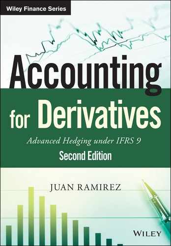
Inflation markets attract a diverse group of participants. In general, these participants can be categorised as inflation payers or receivers (see Figure 12.1).
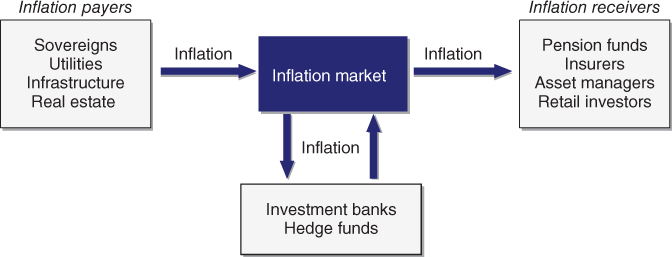
Figure 12.1 Inflation market – main participants.
Inflation Payers
Inflation payers are typically entities with direct or indirect inflation-linked revenues. Inflation is paid predominantly for the purpose of creating financial expenses that match these revenues. Inflation payers include the following:
- Sovereigns. Theoretically, paying inflation can smooth the cash flows of governments as a substantial proportion of governments' incomes are at least partially inflation-linked. For example, value added taxes on gasoline are a function of the price and demand for this commodity. By matching the mix of income and payments, a government can reduce the volatility of its cash flows and, in theory at least, reduce the need to adjust its fiscal policy. In practice sovereigns with large borrowing requirements are the largest issuers of inflation-linked bonds tapping an investor base different from that of fixed rate and floating rate bonds.
- Utility and infrastructure companies. These typically have pricing structures that are statutorily linked to inflation.
- Real estate companies. Rents on commercial investment properties are often periodically adjusted to incorporate inflation. Real estate companies may want to shed some of their revenues' natural exposure to inflation risk by paying inflation.
Inflation Receivers
Inflation receivers have typically been entities aiming to achieve a specific return over inflation and entities incurring costs (e.g., wages) linked to inflation. Inflation receivers include asset managers and pension funds with specific inflation benchmarks and pension funds with pension schemes' liabilities linked to inflation.
- Pension funds and insurance companies. Often these institutional investors offer additional retirement coverage investments and are interested in real returns rather than nominal returns. Investing in inflation-paying securities on their assets side can substantially reduce their liabilities' natural exposure to inflation risk.
- Asset managers. Inflation-linked funds offer investors an asset class that traditionally has shown low correlation to other asset classes such as equities and fixed rates.
- Retail investors. Although most individuals invest in inflation-linked cash flows via their pension schemes, many wealthy investors prefer to additionally invest directly in inflation-linked securities.
Other Market Participants
There are other market participants that do not have a natural exposure to either pay or receive inflation. These include investment banks taking inflation positions to accommodate their clients' inflation hedging needs and hedge funds willing to pay (or receive) inflation when in their view inflation expectations are too high (or low).
12.1.2 Measuring Inflation from Indices
Any inflation-linked instrument needs a reference measure of inflation – a so-called inflation index. This subsection explains what an inflation figure represents and how it is measured from inflation indices.
A (retail) inflation index tries to measure the price of a representative basket of consumer goods and services in a specific country. Every month officials in that country publish a new index level, based on the prices of a basket encompassing hundreds of components. The components of inflation indices and their weights vary from country to country, and include transportation, food and non-alcoholic beverages, clothing and footwear, education, restaurants and hotels, alcohol and tobacco, housing and household goods.
Whilst housing represents one of the largest sources of expenditure for most people, it is much harder to observe than other areas of the index that are directly purchased. For example, the housing component of the UK's Retail Price Index (RPI) tries to incorporate all costs incurred by a homeowner, from mortgage costs to depreciation and council tax.
In itself the level of an inflation index is meaningless, unless it is compared with a previous level. When the price levels of two dates of the same inflation index are compared, a measurement of the increase (or decrease) of the prices in that economy between the two dates is obtained (what is commonly termed as inflation).
A base date is chosen at which the value of the index is set to, say, 100. An index value represents the value of the underlying basket at a point in time (i.e., a certain month/year) assuming that the basket was worth 100 on the base date.
Suppose that the levels of an inflation index associated with March 20X0 and March 20X1 were 130.15 and 135.66, respectively. The annualised inflation rate between those two periods was therefore 4.23% (=135.66/130.15 – 1).
Suppose further that the officials in the country to which the inflation index related reported an inflation figure related for April 20X1 of 4.05%. The published value of the index corresponding to April 20X1 was 136.12 (=135.66 × (1 + 4.05%/12)).
In general, the change in purchasing power between times 0 and t is given by Indext/Index0, where Indext is the value of the index at time t and Index0 is its value at time 0.
12.1.3 Main Inflation Indices
In this subsection I briefly describe the most important inflation indices.
Eurozone Inflation Index
The euro-area inflation derivatives market is arguably the most liquid, active and transparent inflation market. The benchmark index for the eurozone is the Harmonised Index of Consumer Prices (HICP) which measures the price levels of the different eurozone countries. The HICP is a weighted sum of the euro-area countries' HICP indices, weighted to take into account the share of GDP of each country in the overall GDP of the eurozone. The country weights are adapted on an annual basis based on GDP. The item weights of the HICP also vary as a consequence of varying country weights due to the fact that the individual HICP indices have varying item weights. As countries accede to the monetary union, they will be included in the index. Each member state uses the same methodology.
The unrevised HICP excluding tobacco (HICPxT) is used as the reference index in most bonds and derivatives linked to European inflation. HICP is published monthly by Eurostat (www.europa.eu.int/comm/eurostat/). The base year for HICP is 1996, meaning that the average index value of HICP equalled 100 during 1996. HICP is typically published 2 weeks after the end of the month. For instance, the HICPxT index value for March is announced on about 15 April. The index announced is called the unrevised index. Eurostat might revise the index if after gathering more data its officials believe their initial announcement was inaccurate.
Although the value of the index can be revised, the unrevised version is used in both the cash and the derivatives market. The HICPxT index is published by Bloomberg under the ticker CPTFEMU<Index>.
France
When France originally decided to issue inflation-linked debt, there was considerable debate about which index the issues should be linked to. A national index was likely to be a better match to the government's liabilities, while the eurozone HICPxT index appealed to international investors. Given the fact that the latter index was relatively new, the non-seasonally adjusted French Consumer Price Index (CPI) was chosen. The index for each month is published by INSEE (www.insee.fr/en/indicateur/indic_cons/indic_cons.asp) on about the 22nd of the subsequent month. Again the unrevised index is used for both bonds and derivatives. The French CPI is published by Bloomberg under the ticker FRCPXTOB<Index>. The base year is 1998.
United Kingdom
In the UK market, inflation-linked securities are linked to the RPI. The unrevised version is used for inflation swaps. The Office for National Statistics (www.statistics.gov.uk/) publishes the RPI index value for each month on about the 15th of the following month. The Bloomberg ticker for RPI is UKRPI<Index>. The base reference date is January 1987.
United States
The All Items Consumer Price Index for all urban consumers (CPI-U) published by the Bureau of Labor Statistics is used as the reference index for most US inflation-linked bonds and derivatives. The index can be found on Bloomberg under the ticker CPURNSA<Index>. The base is given by the average index of 1982–1984.
12.1.4 Components of a Bond Yield and the Fisher Equation
The value of a debt instrument is driven by its associated yield, which for a currency is a function of the term to maturity of the instrument. Normally for an issuer and a currency, the longer the term to maturity, the higher the yield. The yield of a debt instrument has a number of components (see Figure 12.2) :
- A credit risk premium that takes into account the creditworthiness of the issuer. Normally, longer-term maturities are viewed to have more credit risk than shorter-term maturities.
- A liquidity risk premium that takes into account how deep the market is for the debt instrument. Normally, longer-term maturities are viewed to have more liquidity risk than shorter-term maturities.
- A nominal interest rate which represents a risk-free rate adjusted for expectations and risks related to future inflation during the term of the debt instrument. In theory all bonds of all issuers with the same term to maturity and denominated in the same currency have an identical nominal interest rate.
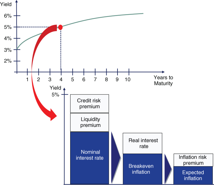
Figure 12.2 Components of a bond yield.
In turn, a nominal interest rate can be broken down into two parts:
- A real interest rate which represents the interest rate in an economy after the effects of inflation have been removed.
- A breakeven inflation component. The breakeven inflation represents the expected inflation during the term of the bond and a premium that compensates investors for the risk of potential changes in inflation expectations.
The Fischer Equation
Because the yield and the sum of the credit risk premium and the liquidity premium of a bond can be directly observed from active markets (e.g., independent quotes may be obtained in the market for credit derivatives), nominal interest rates can be inferred. An interesting debate within the economic community concerns whether real interest rates can be reliably determined. The Fisher equation provides a relationship between nominal interest rates, real interest rates and inflation:
This formula can be approximated as:
where n is the nominal interest rate, r is the real interest rate, and i represents inflation expectations and inflation risk premium.
12.1.5 Breakeven Inflation
As noted previously, the breakeven inflation rate (BEI) in a bond's yield represents the sum of the expected inflation and the inflation risk premium, two components of nominal yields that on their own are not always easily quantifiable. Assuming an inflation risk premium much lower than the expected inflation, a BEI provides a rough measure of inflation expectations.
Assuming an inflation-linked bond (ILB) and a comparable fixed rate bond of the same issuer and liquidity, the BEI equals the difference between the yields of these bonds. If actual inflation is greater than breakeven inflation, the ILB is likely to outperform the fixed rate bond. If actual inflation is lower than breakeven inflation, the fixed rate bond is likely to outperform the ILB. In other words, breakeven inflation is the future inflation rate required for an ILB to achieve the same return as a comparable fixed rate bond, if held to maturity. Thus, investors who wish to take a view on the path of inflation have a choice. If they believe that inflation will be higher than the level priced in by the market, they will sell fixed rate bonds and buy ILBs. If lower, they will do the opposite.
12.2 INFLATION-LINKED BONDS
This section discusses the basics of inflation-linked bonds. It explains key concepts such as real rates and breakeven inflation. ILBs, sometimes known as “linkers” or “real bonds”, are an attractive asset class for investors whose liabilities are linked to inflation, such as insurance companies and pension funds. ILBs are predominantly issued by governments and provide income and total return which adjusts to keep up with the pace of inflation. The UK was the first major market to issue these bonds in 1981 and the US government followed suit by issuing Treasury inflation-protected securities (TIPS) in 1997. Inflation-indexed government bonds are also available in many other countries including Australia, Canada, France, Germany, Italy and Sweden.
The main cash flows in a ILB are as follows (see Figure 12.3):
- On the issue date, the ILB investors pay the bond's initial notional to the issuer (or to the banks intermediating the issuance).
- Periodically, the issuer pays to the investors a fixed coupon on an inflation-adjusted notional amount.
- At maturity, the issuer pays to the investors the initial notional adjusted for inflation.

Figure 12.3 Inflation-linked bond cash flows.
A new ILB is typically issued with an initial notional and a real yield determined through the auction process. Imagine that on 1 January 20X0 a new ILB was issued with a real semiannual coupon of 2%, a initial notional of 100 and a 2-year maturity. The initial consumer price index (Index0) was set at 200, the CPI for October 20W9, 3 months prior to the issue date.
Over time, the notional adjusts according to changes in the CPI from the time the bond is issued. In our example, the adjusted notional amount at time t equalled 100 × Indext/Index0, where Indext is the value of the CPI at time t. Thus, as time passes the redemption value increases in such a way as to keep its inflation-adjusted value at 100. In our example, the redemption amount at maturity was 105.55, calculated adjusting the initial notional of 100 for the change in inflation from its issue date (CPI was 200) to maturity (CPI was 211.1 in October 20X1), or 100 × 211.11/200. In theory, in a deflationary environment the principal repayment amount at maturity could decline below the initial notional. In practice, many ILBs guarantee a “deflation floor” with which they will repay at least the initial notional amount at maturity, no matter what the inflation environment.
The coupon paid in an ILB is the real coupon multiplied by the adjusted notional value. As a result, coupon payments increase over time in an inflationary environment and decrease in a deflationary environment. In our example, the ILB paid a semiannual coupon of 1% (=2%/2) of the adjusted notional amount. Because the adjusted notional on 30 June 20X0 was 101.25, the semiannual coupon paid on that date was 1.01 (=101.25 × 2% /2).
The following table and Figure 12.4 summarise the main cash flows under the ILB.
| 1-Jan-X0 | 30-Jun-X0 | 31-Dec-X0 | 30-Jun-X1 | 31-Dec-X1 | |
| Indext | 200 | 202.5 | 205.3 | 208.4 | 211.1 |
| Index0 | 200 | 200 | 200 | 200 | 200 |
| Indext/Index0 | 1.0125 | 1.0265 | 1.042 | 1.0555 (1) | |
| Adj. notional | 100 | 101.25 | 102.65 | 104.2 | 105.55 (2) |
| Coupon payment | 1.01 | 1.03 | 1.04 | 1.06 (3) | |
| Principal repayment | 105.55 (4) | ||||
| Total cash flow | 1.01 | 1.03 | 1.04 | 106.61 (5) |
Notes:
(1) Indext/Index0 = 211.11/200
(2) Initial notional × Indext/Index0= 100 × 1.0555
(3) Adjusted notional × Coupon rate/2 = 105.55 × 2%/2
(4) Adjusted notional at maturity date
(5) Coupon + Principal repayment = 1.06 + 105.55

Figure 12.4 ILB cash flows.
With the inflation-adjusted value of both the coupon and the notional always preserved, the bond hedged the risk of rising inflation. However, the hedge was slightly imperfect, since the inflation index lagged 3 months.
The accreting nature of ILBs heightens the credit exposure of the investor to the bond issuer. Consequently, the longer the term of the ILB and the larger the inflation, the larger the credit exposure is.
The return on an ILB has two sources of yield: the real yield and a yield representing actual trailing inflation. ILBs are unique in that their real yields are clearly identifiable, and they provide a predictable real return.
12.3 INFLATION DERIVATIVES
The primary purpose of inflation derivatives is the transfer of inflation risk. The advantage of inflation derivative contracts over inflation bonds is that derivatives can be tailored to fit particular client demand more precisely than bonds. Their flexibility also allows them to replicate in derivative form the inflation risks embedded in other instruments such as standard cash instruments (i.e., inflation-linked bonds).
Inflation swaps are the most common inflation derivatives. An inflation swap is a bilateral contract involving the exchange of inflation-linked payments for predetermined fixed or floating payments. It is typically used to hedge inflation risk as it allows entities to swap inflation-linked payments for fixed payments, and vice versa. For example, an entity having inflation-linked revenue streams could swap fixed payments for inflation-linked payments over a predetermined period, effectively creating inflation-linked borrowing. There are a number of instruments that can be classified as inflation derivatives, ranging from zero-coupon inflation swaps to structured inflation products.
There are many types of periodic inflation swaps, and in Sections 12.3.1–12.3.3 I will describe the most common ones, which I have termed zero-coupon, non-cumulative periodic and cumulative periodic inflation swaps. In Section 12.3.4 I turn to inflation caps and floors.
12.3.1 Zero-Coupon Inflation Swaps
Zero-coupon inflation swaps are simple structures that account for a large proportion of the inflation derivatives market, due to their simplicity. These swaps provide a direct measurement of breakeven inflation.
A zero-coupon inflation swap is an agreement between two counterparties in which one party agrees to pay an inflation-linked flow versus a fixed amount, for a given notional amount and period of time. The only cash flows in a zero-coupon swap are paid at maturity (see Figure 12.5): a compounded fixed amount
where X% is the market quoted zero-coupon rate, representing the expected average annual inflation rate over the period, and t is the number of years to maturity; and a realised inflation amount
where IndexFinal and IndexInitial are jointly defined by the payment date, start date and the lag, which is the number of months between the payment date and the month in which IndexFinal is observed. For example, if the payment date is in May, and the lag is 3 months, then IndexFinal is for the month of February.

Figure 12.5 Zero-coupon inflation swap – cash flows.
The following table provides an example of the main terms in a 5-year zero-coupon inflation swap:
| Zero-coupon inflation swap terms | |
| Trade date | 28 October 20X2 |
| Effective date | 1 November 20X2 |
| Maturity date | 1 November 20X7 (5 years) |
| Notional | EUR 100 million |
| Party A receives from party B | Notional × [(1 + 2.50%)5 – 1], paid at maturity date |
| Party A pays to party B | Notional × [(IndexFinal/IndexInitial) – 1], paid at maturity date |
| Index | HICPxT for the eurozone, non-revised, published by Eurostat. For information purposes only, this index is published on Bloomberg page CPTFEMU<Index> |
| IndexInitial | HICP corresponding to the month of August 20X2. IndexInitial was set at 234.5 |
| IndexFinal | HICP corresponding to the month of August 20X7 |
Party A received the fixed amount and paid the inflation amount. The fixed rate was 2.50%, representing the expected annual inflation over the 5-year period. A realised annual inflation rate lower than 2.50%, would result in A receiving a settlement amount at maturity. Conversely, a realised annual inflation rate higher than 2.50% would result in A paying a settlement amount at maturity. The position of B was the opposite of that of A. Party A probably had inflation-linked revenues and through the zero-coupon inflation swap it was protecting itself against an annual European inflation rate lower than 2.50% over the next 5 years, while not benefiting from a potential rise in such inflation above 2.50%. Zero-coupon inflation swaps are also interesting for investors (like B) looking to protect an investment over a certain period against rising inflation rates.
Suppose that the HICP level corresponding to August 20X7 was 285.3. The settlement amount on 1 November 20X7 was calculated as follows: A was due to receive EUR 13,140,821.29 (=100 mn × ((1 + 2.50%)5 – 1)) from B, while A was due to pay EUR 21,663,113.01 (=100 mn × (285.3/234.5 – 1)) to B. Therefore, A paid to B the difference, EUR 8,522,291.72 (=21,663,113.01 – 13,140,821.29), as shown in Figure 12.6.
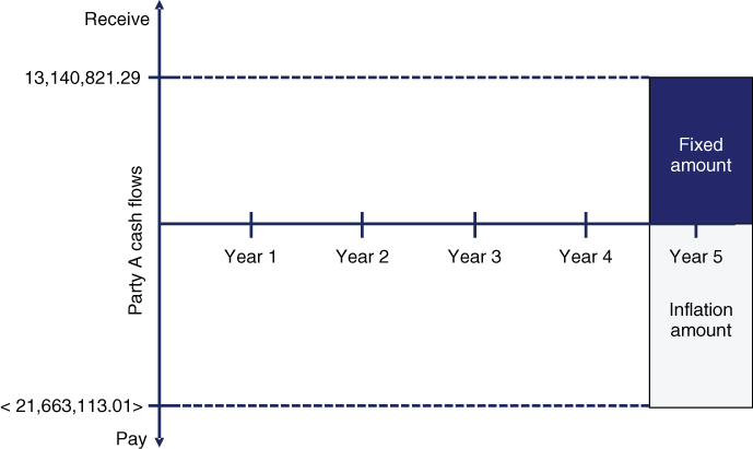
Figure 12.6 Zero-coupon inflation swap – cash flows.
It is important to note that the accreting nature of zero-coupon inflation swaps heightens credit exposure, in the absence of other credit risk mitigants like a collateralised ISDA agreement. In our previous numerical example, A was expected to pay to B over EUR 8.5 million, a substantial amount relative to the notional amount.
12.3.2 Non-cumulative Periodic Inflation Swaps
A periodic inflation swap is an agreement between two counterparties in which one party agrees to periodically swap fixed payments (or floating payments linked to Libor/Euribor rates) for floating payments linked to an inflation rate, for a given notional amount and period of time.
In a non-cumulative periodic inflation swap the notional is not adjusted and as a result the periodic cash flows are calculated over the initial notional (see Figure 12.7), as follows. One party to the swap periodically pays a fixed amount (or a Euribor/Libor based amount)
where X% is a fixed rate, representing the expected average annual inflation rate over the life of the swap. The other party to the swap periodically pays the realised inflation amount during the interest period
where Indext is the inflation index corresponding to the end date of the interest period (taking into account the time lag between such date and the month in which the inflation index is observed) and Indext–1 is the inflation index corresponding to the end date of the previous interest period.

Figure 12.7 Non-cumulative inflation swap – cash flows.
The following table provides an example of the main terms of a 5-year non-cumulative inflation swap with a 3% fixed rate and a notional amount.
| Periodic non-cumulative inflation swap terms | |
| Trade date | 28 October 20X2 |
| Effective date | 1 November 20X2 |
| Maturity date | 1 November 20X7 (5 years) |
| Notional | EUR 100 million |
| Party A pays | Notional × 3.00%, paid annually on 1 November |
| Party B pays | Notional × [(Indext/Indext–1) – 1], paid annually on 1 November |
| Index | HICPxT for the eurozone, non-revised, published by Eurostat. For information purposes only, this index is published on Bloomberg page CPTFEMU<Index> |
| Indext | HICP corresponding to the month of August of the year of the Party B payment date |
| Indext–1 | Indext corresponding to the previous payment date. For the initial payment date, Indext–1 shall be IndexInitial |
| IndexInitial | 234.5 |
The following table provides a numerical example of the inflation swap settlement amounts, from party A's perspective, based on an assumed scenario of the inflation index (amounts in EUR millions). Because each year the annual inflation was larger than the 3% fixed rate, A received each year a settlement amount that represented the excess of the annual inflation relative to the 3% fixed rate (see Figure 12.8).
| 1-Nov-X3 | 1-Nov-X4 | 1-Nov-X5 | 1-Nov-X6 | 1-Nov-X7 | |
| Indext | 242.6 | 253.7 | 263.4 | 275.4 | 285.3 |
| Indext–1 | 234.5 | 242.6 | 253.7 | 263.4 | 275.4 |
| Indext/Indext–1 – 1 | 0.0345 | 0.0458 | 0.0382 | 0.0456 | 0.0359 |
| Inflation leg amount | 3.45 | 4.58 | 3.82 | 4.56 | 3.59 |
| Fixed leg amount | <3> | <3> | <3> | <3> | <3> |
| Settlement amount | 0.45 | 1.58 | 0.82 | 1.56 | 0.59 |
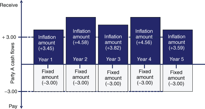
Figure 12.8 Non-cumulative periodic inflation swap – cash flows.
12.3.3 Cumulative Periodic Inflation Swaps
In a cumulative inflation swap the notional on the inflation leg is adjusted and as a result the periodic cash flows are calculated over the initial notional (see Figure 12.9). A cumulative inflation swap is equivalent to a string of zero-coupon inflation swaps, as follows. One party to the swap periodically pays a fixed amount (or a Euribor/Libor based amount):
where X% is a fixed rate. The other party periodically pays the realised inflation amount during the interest period:
where Indext is the inflation index corresponding to the end date of the interest period (taking into account the time lag between such date and the month in which the inflation index is observed) and IndexInitial is the inflation index corresponding to the effective date (taking into account the corresponding time lag).

Figure 12.9 Cumulative periodic inflation swap – cash flows.
The following table provides an example of the main terms in a 5-year cumulative inflation swap with a 3% fixed rate.
| Periodic cumulative inflation swap terms | |
| Trade date | 28 October 20X2 |
| Effective date | 1 November 20X2 |
| Maturity date | 1 November 20X7 (5 years) |
| Notional | EUR 100 million |
| Party A pays | Notional × [(1 + 3.00%)t – 1], paid annually on 1 November t: number of years between the effective date and party A payment date |
| Party B pays | Notional × [(Indext/IndexInitial) – 1], paid annually each 1 November |
| Index | HICPxT for the eurozone, non-revised, published by Eurostat. For information purposes only, this index is published on Bloomberg page CPTFEMU<Index> |
| IndexInitial | HICP corresponding to the month of August 20X2 IndexInitial was set at 234.5 |
| Indext | HICP corresponding to the month of August of the year of the party B payment date |
The following table provides a numerical example of the inflation swap settlement amounts, from party A's perspective, based on an assumed scenario of the inflation index (amounts in EUR millions). Because each year the annual inflation was higher than the 3% fixed rate, A received each year a settlement amount that represented the excess of the cumulative annual inflation relative to the 3% fixed rate (see Figure 12.10). The compounding effect amplified the difference over time, resulting in an increasing settlement amount.
| 1-Nov-X3 | 1-Nov-X4 | 1-Nov-X5 | 1-Nov-X6 | 1-Nov-X7 | |
| Indext | 242.6 | 253.7 | 263.4 | 275.4 | 285.3 |
| IndexInitial | 234.5 | 234.5 | 234.5 | 234.5 | 234.5 |
| Indext/IndexInitial – 1 | 0.034542 | 0.081876 | 0.123241 | 0.174414 | 0.216631 |
| Inflation leg amount | 3.45 | 8.19 | 12.32 | 17.44 | 21.66 |
| Fixed leg amount | <3.00> | <6.09> | <9.27> | <12.55> | <15.93> |
| Settlement amount | 0.45 | 2.10 | 3.05 | 4.89 | 5.73 |
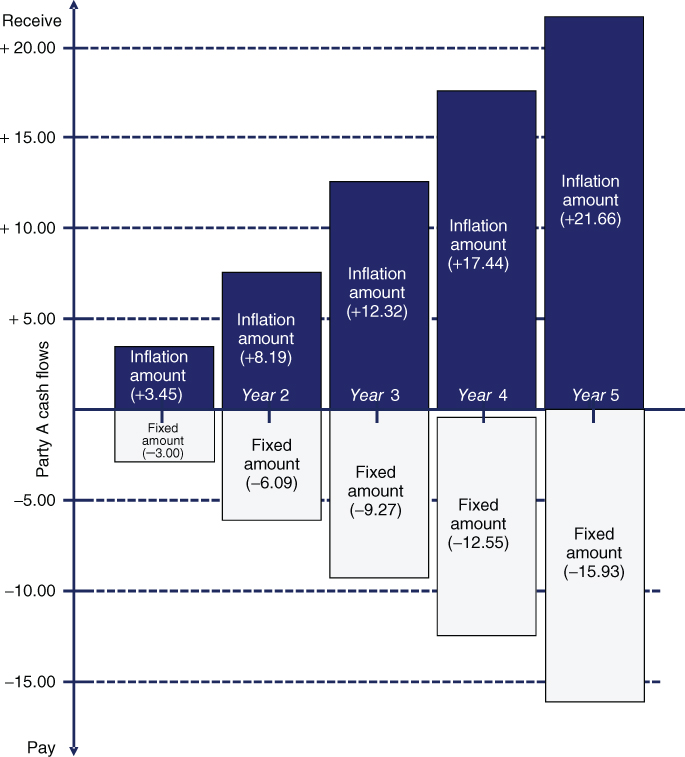
Figure 12.10 Cumulative periodic inflation swap – cash flows.
12.3.4 Inflation Caps and Floors
Besides swaps, options can also be traded on inflation indices. An inflation cap is an option (or a string of options, called caplets) that provides a cash flow equal to the difference between inflation and a pre-agreed strike rate if this difference is positive. An inflation floor is an option (or a string of options, called floorlets) that provides a cash flow equal to the difference between a pre-agreed strike rate and inflation if this difference is positive. Caps and floors play a natural role in hedges of an interval of inflation exposures. For instance, a floor on the principal is often included in inflation-linked bonds in order to protect investors against deflation and/or low inflation rates.
Cumulative or Zero-Coupon Inflation Caps and Floors
Before moving on to periodic caps and floors I cover the simplest of the inflation options: caps and floors on cumulative (also called zero-coupon) inflation. A cumulative inflation floor pays the difference with respect to a (compounded) strike in case inflation turns out to be lower than a pre-specified strike. Floors on cumulative inflation are often embedded in inflation-linked bonds or swaps where principal redemption is floored at par. For instance, all the US TIPS and French government OATis bonds have a redemption-protecting floor guaranteeing redemption equal to par. The following table highlights the main terms of a 3-year 1% cumulative inflation floor that protected the buyer against a 3-year average inflation (i.e., the cumulative inflation over 3 years) below 1%:
| Cumulative inflation floor terms | |
| Trade date | 28 October 20X2 |
| Effective date | 1 November 20X2 |
| End date | 1 November 20X5 (3 years) |
| Notional | EUR 100 million |
| Buyer | Party A |
| Up-front premium | Party A pays 0.21% of the notional (i.e., EUR 210,000) on the effective date |
| Party B pays | Notional × max[(1+1.00%)3 – (IndexFinal/IndexInitial), 0)], paid on end date |
| Index | HICPxT for the eurozone, non-revised, published by Eurostat. For information purposes only, this index is published on Bloomberg page CPTFEMU<Index> |
| IndexInitial | HICP corresponding to the month of August 20X2 IndexInitial was set at 234.5 |
| IndexFinal | HICP corresponding to the month of August 20X5 |
The following table provides an example of the payoff under the floor after a deflationary 3-year period. In this example the average annual inflation was negative (–2.5%), and as a result, party A was compensated for the deficit relative to a 1% average inflation. Thus, on 1 November 20X5 party B paid EUR 10,365,000 to party A.
| 1-Nov-X5 | |
| IndexFinal | 217.3 |
| IndexInitial | 234.5 |
| IndexFinal/IndexInitial | 0.92665 (1) |
| max(1.013 – IndexFinal/IndexInitial, 0) | 10.365% (2) |
| Party B payment to Party A (EUR) | 10,365,000 (3) |
Notes:
(1) 217.3/234.5
(2) Maximum of (1.013 – 0.92665) and zero10.365% × 100,000,000
Periodic Inflation Caps and Floors
In a periodic inflation cap (floor) the buyer is protected periodically against inflation exceeding (underperforming) a certain level, the cap rate (floor rate). A cap (floor) that has more than one exercise date is a combination of several single options called caplets (floorlets). The following table summarises the main terms of a 3-year 4% inflation cap that protected the buyer against an annual inflation rate above 4% (see Figure 12.11). For the protection, party A paid on 1 November 20X2 a EUR 210,000 premium.
| Annual inflation cap terms | |
| Trade date | 28 October 20X2 |
| Effective date | 1 November 20X2 |
| End date | 1 November 20X5 (3 years) |
| Notional | EUR 100 million |
| Buyer | Party A |
| Up-front premium | Party A pays 0.21% of the notional (i.e., EUR 210,000) on the Effective date |
| Party B pays | Notional × max[(Indext/Indext–1) – (1+4.00%), 0)] |
| Party B payment dates | Every 1 November from, and including, 1 November 20X3 up to, and including, the end date |
| Index | HICPxT for the eurozone, non-revised, published by Eurostat. For information purposes only, this index is published on Bloomberg page CPTFEMU<Index> |
| Indext–1 | Indext corresponding to the party B previous payment date Indext–1 for the party B first payment date was set at 234.5 (HICP corresponding to the month of August 20X2) |
| Indext | HICP corresponding to the month of August of the year of the party B payment date |
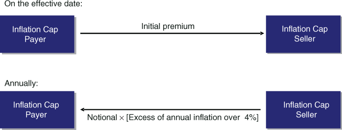
Figure 12.11 Annual inflation cap – cash flows.
The following table provides an example of the payoffs under the cap. In this example the year-on-year inflation for the first year was 4.733% (=245.6/234.5 – 1), and, as a result, the excess of the annual inflation over 4% was 0.733%. Thus, on 1 November 20X3 party B paid EUR 733,000 (i.e., the 0.733% excess inflation over the EUR 100 million notional) to party A. During the second year, annual inflation was 3.094% (=253.2/245.6 – 1), below 4%, and therefore A did not receive any compensation under the cap. During the third year, annual inflation was 6.003% (=268.4/253.2 – 1) exceeding 4%, and thus A received EUR 2,003,000 in compensation.
| 1-Nov-X3 | 1-Nov-X4 | 1-Nov-X5 | |
| Indext | 245.6 | 253.2 | 268.4 |
| Indext–1 | 234.5 | 245.6 | 253.2 |
| Indext/Indext–1 | 1.04733 | 1.03094 | 1.06003 (1) |
| max(Indext/Indext–1 – 1.04 , 0) | 0.733% | 0% | 2.003% (2) |
| Party B payment (EUR) | 733,000 | -0- | 2,003,000 (3) |
Notes:
(1) 268.4/253.2
(2) Maximum of (1.06003 – 1.04) and zero
(3) 2.003% × 100,000,000
12.4 INFLATION RISK UNDER IFRS 9
This section explains some of the accounting issues when inflation is involved.
12.4.1 Hybrid Instruments
Suppose that ABC is Germany-based company with the EUR as its functional (and presentation) currency. ABC issued inflation-linked debt denominated in EUR in which payments of principal and interest are linked to an inflation index. The inflation link is not leveraged and the principal is protected.
Recall from Section 1.6 that when a financial liability encompasses a combination of a host contract and an embedded derivative (a “hybrid instrument”), the issuer needs to assess whether the embedded derivative should be accounted for separately. IFRS 9 does not require the separation of the embedded derivative (see 1.7):
- If the derivative does not qualify as a derivative if it were free-standing. In our example, the inflation-linked feature qualified as a derivative if it was separated from the liability; or
- If the host contract is accounted for at fair value, with changes in fair value recorded in profit and loss. In our example, the host contract was recognised at amortised cost; or
- If the economic characteristics and risks of the embedded derivative are closely related to those of the host contract. This was the key element affecting the assessment. Let us take a look to different inflation underlyings:
- European CPI. This inflation index is the one commonly used in the EUR currency economic environment. Therefore there was no need to separate (the instrument was treated as a liability in its entirety).
- German CPI. Same conclusion as for the European CPI if a sufficiently high correlation can be demonstrated between European and German inflation.
- British RPI. The inflation index relates to a different economic environment. Thus, ABC would need to split the bond into a host contract and a derivative.
In our example, the bond was principal protected. IFRS 9 does not address whether an inflation-linked bond not requiring separation must be principal protected to be eligible for amortised cost recognition. A prolonged deflationary economy may cause a principal unprotected bond to be redeemed below its initial nominal amount, and the accounting community regards the bond as having cash flows that are solely payments of principal and interest on the principal outstanding.
Also, in our example the inflation adjustment was not leveraged. Imagine that instead the adjustment each year was for three times the CPI. In this case, the embedded inflation derivative would be accounted for separately. However, it is less clear whether the separation is the three-times adjustment or just the leveraged part (i.e., a two-times adjustment). However, it is generally understood that splitting the embedded derivative into two derivatives is not generally permitted under IFRS 9, and as a result, the full inflation adjustment (i.e., three times CPI) should be separated.
12.4.2 Hedging Inflation as a Risk Component
Can the inflation component (or “risk portion”) of a fixed or variable interest rate instrument be designated as the risk being hedged in a hedging relationship? Whilst the main requirement is that the portion of a risk has to be identifiable and separately measurable, answering this question may require careful judgement of relevant facts and circumstances.
In principle, inflation may only be hedged when changes in inflation constitute a contractually specified portion of cash flows of a recognised financial instrument. This may be the case where an entity acquires or issues inflation-linked debt. In such circumstances, the entity has a cash flow exposure to changes in future inflation that may be cash flow hedged.
In principle, an entity is not permitted to designate an inflation component which is not contractually specified. For example, IFRS 9 does not deem separately identifiably and reliably measurable the inflation component of issued or acquired fixed rate debt in a fair value hedge. However, for financial instruments, IFRS 9 introduces a rebuttable presumption, meaning that there are limited cases under which it is possible to identify a risk component for inflation and designate that inflation component in a hedging relationship, even though the inflation component is not contractually specified. The assessment is based on the particular circumstances in the related debt market. The following is taken from the application guidance of IFRS 9 (B6.3.14):
For example, an entity issues debt in an environment in which inflation-linked bonds have a volume and term structure that results in a sufficiently liquid market that allows constructing a term structure of zero-coupon real interest rates. This means that for the respective currency, inflation is a relevant factor that is separately considered by the debt markets. In those circumstances the inflation risk component could be determined by discounting the cash flows of the hedged debt instrument using the term structure of zero-coupon real interest rates (i.e., in a manner similar to how a risk-free (nominal) interest rate component can be determined).
In the case of eurozone countries, IFRS 9 does not provide guidance on whether the analysis of inflation as eligible risk component has to be done by analysing the inflation market of the country or the overall inflation for the currency. In my opinion, when a bond is denominated in EUR, the relevant market structure for inflation should be eurozone inflation.
12.5 CASE STUDY: HEDGING REVENUES LINKED TO INFLATION
One of the uses of inflation derivatives is to match inflation-linked revenues with fixed rate funding. Entities exposed to inflation risk and with substantial funding needs may access different investor bases and hedge their inflation risk separately, lowering their cost of funding. The aim of this case study is to illustrate the application of a cash flow hedge of a string of highly expected inflation-linked revenues.
12.5.1 Background
Imagine that in 20X0, ABC – a British toll road operator – signed a 15-year contract with the British government to operate from 1 January 20X1 a highway that had just been constructed. Although both parties to the contract expected their collaboration to last 15 years, every 5 years the British government had the right to renegotiate the contract if the quality of maintenance of the highway was considered to be below a certain standard.
The contract established a cash cost price per vehicle of GBP 4.00 for the calendar year 20X1. The contract included a price adjustment mechanism that provided customers with a fixed “real” price. The price that ABC charged vehicles travelling through its highway was adjusted every 1 January to incorporate the most recent yearly inflation using the British RPI. For example, as shown in Figure 12.12, the price for the year 20X2 would be set by taking the price set for year 20X0 (GBP 4.00) and adjusting it for the inflation rate from October 20X0 to October 20X1. Assuming that the levels of the RPI corresponding to October 20X0 and October 20X1 were 134.1 and 139.8 respectively, implying a 4.28% annualised inflation rate, the price for the year 20X2 would be GBP 4.17 (=4.00 × (1 + 139.8/134.1)).
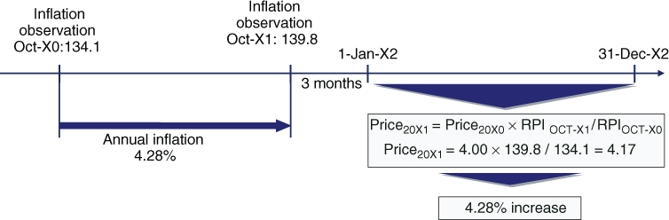
Figure 12.12 Annual reset mechanism of toll price.
By far the largest item affecting ABC's costs was financing expense, which stemmed from interest payments under a 15-year fixed rate loan. Because the revenues were linked to inflation while costs were fixed, ABC hedged the mismatch by entering into a 4-year inflation-linked swap (ILS) with the following terms:
| Inflation swap terms | |
| Trade date | 1 January 20X1 |
| Effective date | 31 December 20X1 |
| Counterparties | ABC and XYZ Bank |
| Nominal amount | GBP 146 million |
| Termination date | 31 December 20X5 (4 years) |
| ABC receives | Notional × [(1 + 3.71%)t – 1], paid annually on 31 December, starting on 31 December 20X2 t: number of years between the effective date and ABC payment date |
| ABC pays | Notional × [(Indext/IndexInitial) – 1], paid annually on 31 December, starting on 31 December 20X2 |
| Index | British non-revised RPI |
| IndexInitial | The index for the month of October 20X0 which was 134.1 |
| IndexFinal | The index for the reference month of October preceding ABC payment date |
Under the ILS, each year ABC paid the realised inflation and received a fixed rate of 3.71%, accrued since the effective date (see Figure 12.13). Thus, on a notional of GBP 146 million and assuming a constant amount of traffic, ABC locked in revenues growing at a 3.71% annual rate. The GBP 146 million notional represented the expected revenues for the year 20X1 (i.e., 36.5 million vehicles times GBP 4.00). Whilst ABC was exposed to a lower than expected volume of traffic, it concluded that 36.5 million vehicles was a reliable estimate.

Figure 12.13 Inflation-linked swap annual cash flows.
12.5.2 Hedging Relationship Documentation
ABC designated the ILS as the hedging instrument in a cash flow hedging relationship of a string of four highly expected cash flows. In order to justify the high probability of occurrence of the cash flows ABC produced an analysis in which it substantiated that traffic of 36.5 million vehicles was a conservative estimate and described the pricing mechanism formalised under the contract with the British authorities.
| Hedging relationship documentation | |
| Risk management objective and strategy for undertaking the hedge | The objective of the hedge is to protect the GBP value of the highly expected cash flows stemming from the operation of a toll road for 4 years. This hedging objective is consistent with the entity's risk management strategy of reducing the variability of its profit or loss statement caused by inflation-linked revenues with inflation-linked swaps and debt. The designated risk being hedged is the risk of changes in the GBP value of the highly expected cash flows due to unfavourable movements in the British RPI rate |
| Type of hedge | Cash flow hedge |
| Hedged item | The hedged item is the yearly high expected cash flows stemming from the contract to operate highway E-106, from 1 January 20X2 to 31 December 20X5, corresponding to a forecasted annual traffic of 36.5 million vehicles. These cash flows are highly probable as the forecasted annual traffic is considered to be very conservative, and the pricing mechanism has been formalised through a contract with the British government |
| Hedging instrument | The inflation-linked swap contract with reference number 012845. The counterparty to the ILS is XYZ Bank and the credit risk associated with this counterparty is considered to be very low. The ILS contract has a GBP 146 million notional, an effective date of 31 December 20X1 and a maturity date of 31 December 20X5. Yearly settlement amounts will be paid/received as the net of (i) the entity paying the cumulative inflation since the effective date on the notional and (ii) the entity receiving a cumulative amount yielding an annual 3.71% fixed rate since the effective date on the notional |
| Hedge effectiveness assessment | See below |
12.5.3 Hedge Effectiveness Assessment – Hypothetical Derivative
Although the cash flows take place almost evenly during the year, for assessment purposes they will be grouped into one flow taking place at the end of the year. Hedge effectiveness will be assessed by comparing changes in the fair value of the hedging instrument to changes in the fair value of a hypothetical derivative. The terms of the hypothetical derivative – an ILS with nil fair value at the start of the hedging relationship – reflected the terms of the hedged item. The terms of the hypothetical derivative were identical to those of the hedging instrument except the counterparty to ILS which was assumed to be credit risk-free and a fixed rate of 3.70%.
Note that the fixed rate of the hypothetical derivative (3.70%) was different from that of the hedging instrument (3.71%) due to the absence of CVA in the hypothetical derivative (the counterparty to the hypothetical derivative was assumed to be credit risk-free).
Changes in the fair value of the hedging instrument will be recognised as follows:
- The effective part of the gain or loss on the hedging instrument will be recognised in the cash flow hedge reserve of OCI. The accumulated amount in equity will be reclassified to profit or loss in the same period during which the hedged expected future cash flow affects profit or loss, adjusting the sales amount.
- The ineffective part of the gain or loss on the hedging instrument will be recognised immediately in profit or loss.
Hedge effectiveness will be assessed prospectively at hedging relationship inception, on an ongoing basis at each reporting date and upon occurrence of a significant change in the circumstances affecting the hedge effectiveness requirements.
The hedging relationship will qualify for hedge accounting only if all the following criteria are met:
- The hedging relationship consists only of eligible hedge items and hedging instruments. The hedge item is eligible as it is a string of highly expected forecast transactions exposing the entity's profit or loss to fair value risk and is reliably measurable. The hedging instrument is eligible as it is a derivative and it does not result in a net written option.
- At hedge inception there is a formal designation and documentation of the hedging relationship and the entity's risk management objective and strategy for undertaking the hedge.
- The hedging relationship is considered effective.
The hedging relationship will be considered effective if all the following requirements are met:
- There is an economic relationship between the hedged item and the hedging instrument.
- The effect of credit risk does not dominate the value changes that result from that economic relationship.
- The hedge ratio of the hedging relationship is the same as that resulting from the quantity of hedged item that the entity actually hedges and the quantity of the hedging instrument that the entity actually uses to hedge that quantity of hedged item. The hedge ratio should not be intentionally weighted to create ineffectiveness.
Whether there is an economic relationship between the hedged item and the hedging instrument will be assessed on a qualitative basis. The assessment will be complemented by a quantitative assessment using the scenario analysis method for one scenario in which the expected inflation rates will be calculated by shifting the expected inflation rates prevailing on the assessment date by +2%, and the change in fair value of both the hypothetical derivative and the hedging instrument compared.
12.5.4 Hedge Effectiveness Assessment Performed at Start of the Hedging Relationship
ABC performed an effectiveness assessment on 1 January 20X1, the start date of the hedging relationship, which was documented as follows.
The hedging relationship was considered effective as all the following requirements were met:
- There was an economic relationship between the hedged item and the hedging instrument. Based on the qualitative assessment performed supported by a quantitative analysis, the entity concluded that the change in fair value of the hedged item was expected to be substantially offset by the change in fair value of the hedging instrument, corroborating that both elements had values that would generally move in opposite directions.
- The effect of credit risk did not dominate the value changes resulting from that economic relationship as the credit ratings of both the entity and XYZ Bank were considered sufficiently strong.
- The 1:1 hedge ratio of the hedging relationship was the same as that resulting from the quantity of hedged item that the entity actually hedged and the quantity of the hedging instrument that the entity actually used to hedge that quantity of hedged item. The hedge ratio was not intentionally weighted to create ineffectiveness.
Due to the fact that the main terms of the hedging instrument and those of the expected cash flow closely matched and the low credit risk exposure to the counterparty of the ILS contract, it was concluded that the hedging instrument and the hedged item had values that would generally move in opposite directions. This conclusion was supported by a quantitative assessment, which consisted of one scenario analysis performed as follows. The expected inflation rates on the assessment date were simulated by shifting on a parallel basis the expected inflation rates prevailing on the assessment date by +2%. As shown in the table below, the change in fair value of the hedged item was expected to largely be offset by the change in fair value of the hedging instrument, corroborating that both elements had values that would generally move in opposite directions.
| Scenario analysis assessment | ||
| Hedging instrument | Hypothetical derivative | |
| Initial fair value | Nil | Nil |
| Final fair value | <24,472,000> | <24,592,000> |
| Cumulative fair value change | <24,472,000> | <24,592,000> |
| Degree of offset | 99.5% | |
The hedge ratio was set at 1:1, resulting from the GBP 146 million quantity of hedged item that the entity actually hedged and the GBP 146 million quantity of the hedging instrument that the entity actually used to hedge that quantity of hedged item. The hedge ratio was not intentionally weighted to create ineffectiveness.
The following sources of ineffectiveness were identified: a change in the estimated cash flows below the hedged notional, a substantial deterioration of the creditworthiness of the counterparty to the ILS and changes in the agreement with the British government.
ABC also performed an effectiveness assessment on each reporting date, yielding very similar results, which have been omitted to avoid unnecessary repetition.
12.5.5 Fair Valuations of the ILS and the Hypothetical Derivative
The following table details the fair valuation of the hedging instrument on 1 January 20X1:
| Hedging instrument fair valuation on 1 January 20X1 | |||||||
| Cash flow date | Discount factor (1) | Expected inflation rate (2) | Expected RPI (3) | Inflation leg cash flow (4) | Fixed leg cash flow (5) | Expected settlement amount (6) | Present value (7) |
| 31-Dec-X2 | 0.8972 | 4.22% | 139.8 | <6,206,000> | 5,417,000 | <789,000> | <708,000> |
| 31-Dec-X3 | 0.8458 | 3.45% | 144.6 | <11,432,000> | 11,034,000 | <398,000> | <337,000> |
| 31-Dec-X4 | 0.7950 | 3.30% | 149.4 | <16,658,000> | 16,860,000 | 202,000 | 161,000 |
| 31-Dec-X5 | 0.7466 | 3.10% | 154.0 | <21,666,000> | 22,902,000 | 1,236,000 | 923,000 |
| CVA/DVA | <39,000> | ||||||
| Total | -0- | ||||||
Notes:
(1) Discount factor, between 31-Jan-X1 (valuation date) and the cash flow date calculated using the GBP Libor curve
(2) Expected inflation rate from previous year's October to October of the year of the cash flow. For example, 4.22% was the expected inflation rate from October 20X0 to October 20X1
(3) The level of the British RPI index assuming a level of 134.1 for the month of October 20X0. For example, 139.8 = 134.1 × (1 + 4.22%), rounded to one decimal place
(4) <GBP 146 mn> × (Previous RPI/Current RPI − 1). For example, <6,206,000> = <146 mn> × (139.8/134.1 − 1)
(5) GBP 146 mn × [(1+3.71%)Years − 1], where Years was the number of calendar years since the effective date (31 December 20X1). For example, 11,034,000 = 146 mn × [(1+3.71%)2 – 1]
(6) Inflation leg cash flow + Fixed leg cash flow. For example, <789,000> = <6,206,000> + 5,417,000
(7) Settlement amount × Discount factor. For example, <708,000> = <789,000> × 0.8972
The following table details the fair valuation of the hedging instrument on 31 December 20X1:
| Hedging instrument fair valuation on 31 December 20X1 | |||||||
| Cash flow date | Discount factor | Expected inflation rate | Expected RPI (*) | Inflation leg cash flow | Fixed leg cash flow | Expected settlement amount | Present value |
| 31-Dec-X2 | 0.9481 | 4.28% | 139.8 | <6,206,000 | 5,417,000 | <789,000> | <748,000> |
| 31-Dec-X3 | 0.8963 | 3.60% | 144.8 | <11,650,000> | 11,034,000 | <616,000> | <552,000> |
| 31-Dec-X4 | 0.8449 | 3.45% | 149.8 | <17,093,000> | 16,860,000 | <233,000> | <197,000> |
| 31-Dec-X5 | 0.7934 | 3.25% | 154.7 | <22,428,000> | 22,902,000 | 474,000 | 376,000 |
| DVA | 34,000 | ||||||
| Total | <1,087,000> | ||||||
(*) RPI corresponding to October 20X1 was 139.8
The following table details the fair valuation of the hedging instrument on 31 December 20X2:
| Hedging instrument fair valuation on 31 December 20X2 | |||||||
| Cash flow date | Discount factor | Expected inflation rate | Expected RPI (*) | Inflation leg cash flow | Fixed leg cash flow | Expected settlement amount | Present value |
| 31-Dec-X3 | 0.9554 | 4.70% | 145.0 | <11,867,000> | 11,034,000 | <833,000> | <796,000> |
| 31-Dec-X4 | 0.9115 | 3.30% | 149.8 | <17,093,000> | 16,860,000 | <233,000> | <212,000> |
| 31-Dec-X5 | 0.8675 | 3.20% | 154.6 | <22,319,000> | 22,902,000 | 583,000 | 506,000> |
| DVA | 8,000 | ||||||
| Total | <494,000> | ||||||
(*) RPI corresponding to October 20X2 was 145.0
The following table details the fair valuation of the hedging instrument on 31 December 20X3:
| Hedging instrument fair valuation on 31 December 20X3 | |||||||
| Cash flow date | Discount factor | Expected inflation rate | Expected RPI (*) | Inflation leg cash flow | Fixed leg cash flow | Expected settlement amount | Present value |
| 31-Dec-X4 | 0.9700 | 2.10% | 148.0 | <15,133,000> | 16,860,000 | 1,727,000 | 1,675,000 |
| 31-Dec-X5 | 0.9404 | 2.20% | 151.3 | <18,726,000> | 22,902,000 | 4,176,000 | 3,927,000 |
| CVA | <56,000> | ||||||
| Total | 5,546,000 | ||||||
(*) RPI corresponding to October 20X3 was 148.0
The following table details the fair valuation of the hedging instrument on 31 December 20X4:
| Hedging instrument fair valuation on 31 December 20X4 | |||||||
| Cash flow date | Discount factor | Expected inflation rate | Expected RPI (*) | Inflation leg cash flow | Fixed leg cash flow | Expected settlement amount | Present value |
| 31-Dec-X5 | 0.9772 | 1.80% | 150.7 | <18,073,000> | 22,902,000 | 4,829,000 | 4,719,000 |
| CVA | <24,000> | ||||||
| Total | 4,695,000 | ||||||
(*) RPI corresponding to October 20X4 was 150.7
The fair valuation of the hypothetical derivative was similar to that of the hedging instrument. The only differences were the fixed leg cash flows (which were computed based on a 3.70% fixed rate) and the absence of CVA (DVA remained present).
The following table summarises the fair values of the hedging instrument and the hypothetical derivative at each relevant date:
| Date | Hedging instrument fair value | Period change | Cumulative change | Hypothetical derivative value | Cumulative change |
| 1-Jan-X1 | -0- | — | — | -0- | — |
| 31-Dec-X1 | <1,087,000> | <1,087,000> | <1,087,000> | <1,215,000> | <1,215,000> |
| 31-Dec-X2 | <494,000> | 593,000 | <494,000> | <622,000> | <622,000> |
| 31-Dec-X3 | 5,546,000 | 6,040,000 | 5,546,000 | 5,496,000 | 5,496,000 |
| 31-Dec-X4 | 4,695,000 | <851,000> | 4,695,000 | 4,655,000 | 4,655,000 |
| 31-Dec-X5 | -0- | <4,695,000> | -0- | -0- | -0- |
The ineffective part of the change in fair value of the hedging instrument was the excess of its cumulative change in fair value over that of the hypothetical derivative. The effective and ineffective parts of the period change in fair value of the ILS were the following (see Section 5.5.6 for an explanation of the calculations):
| 31-Dec-X1 | 31-Dec-X2 | 31-Dec-X3 | 31-Dec-X4 | 31-Dec-X5 | |
| Cumulative change in fair value of hedging instrument | <1,087,000> | <494,000> | 5,546,000 | 4,695,000 | -0- |
| Cumulative change in fair value of hypothetical derivative | <1,215,000> | <622,000> | 5,496,000 | 4,655,000 | -0- |
| Lower amount | <1,087,000> | <494,000> | 5,496,000 | 4,655,000 | -0- |
| Sum of previous effective parts | — | <1,087,000> | <494,000> | 5,496,000 | 4,655,000 |
| Available amount | <1,087,000> | 593,000 | 5,990,000 | <841,000> | <4,655,000> |
| Period change in fair value of hedging instrument | <1,087,000> | 593,000 | 6,040,000 | <851,000> | <4,695,000> |
| Effective part | <1,087,000> | 593,000 | 5,990,000 | <841,000> | <4,655,000> |
| Ineffective part | -0- | -0- | 50,000 | <10,000> | <40,000> |
The following table summarises the settlement amounts under the ILS:
| Date | Actual inflation | RPI level | ILS settlement amount |
| 31-Dec-X2 | 4.28% | 139.8 | <789,000> |
| 31-Dec-X3 | 4.70% | 145.0 | <833,000> |
| 31-Dec-X4 | 2.10% | 148.0 | 1,727,000 |
| 31-Dec-X5 | 1.80% | 150.7 | 4,829,000 |
The following table summarises the revenues generated by ABC, assuming that the actual annual traffic was exactly 36.5 million vehicles:
| Year Ending | Traffic | Price | Revenue |
| 31-Dec-X1 | 36.5 mn | 4.000 | 146,000,000 |
| 31-Dec-X2 | 36.5 mn | 4.170 | 152,205,000 |
| 31-Dec-X3 | 36.5 mn | 4.325 | 157,863,000 |
| 31-Dec-X4 | 36.5 mn | 4.414 | 161,111,000 |
| 31-Dec-X5 | 36.5 mn | 4.495 | 164,068,000 |
12.5.6 Accounting Entries
Suppose that ABC reported financially every 31 December.
- Accounting entries on 1 January 20X1
No entries were required as the fair value of the swap was nil on trade date.
- Accounting entries on 31 December 20X1
ABC recognised GBP 146 million revenues for the year, which were received in cash. The change in fair value of the ILS produced a GBP 1,087,000 loss, fully deemed to be effective and recorded in the cash flow hedge reserve of OCI.
- Accounting entries on 31 December 20X2
ABC recognised GBP 152,205,000 revenues for the year, which were received in cash. ABC paid GBP 789,000 under the ILS and adjusted the revenues figure. The change in fair value of the ILS produced a GBP 593,000 gain, fully deemed to be effective and recorded in the cash flow hedge reserve of OCI.
- Accounting entries on 31 December 20X3ABC recognised GBP 157,863,000 revenues for the year, which were received in cash. ABC paid GBP 833,000 under the ILS and adjusted the revenues figure. The change in fair value of the ILS produced a GBP 6,040,000 gain, of which GBP 5,990,000 was deemed to be effective and recorded in the cash flow hedge reserve of OCI, while GBP 50,000 was considered to be ineffective and recorded in profit or loss.
- Accounting entries on 31 December 20X4
ABC recognised GBP 161,111,000 revenues for the year, which were received in cash. ABC received GBP 1,727,000 under the ILS and adjusted the revenues figure. The change in fair value of the ILS produced a GBP 851,000 loss, of which GBP <841,000> was deemed to be effective and recorded in the cash flow hedge reserve of OCI, while GBP <10,000> was considered to be ineffective and recorded in profit or loss.
- Accounting entries on 31 December 20X5
ABC recognised GBP 164,068,000 revenues for the year, which were received in cash. ABC received GBP 4,829,000 under the ILS and adjusted the revenues figure. The change in fair value of the ILS produced a GBP 4,695,000 loss, of which GBP <4,655,000> was deemed to be effective and recorded in the cash flow hedge reserve of OCI, while GBP <40,000> was considered to be ineffective and recorded in profit or loss.
12.5.7 Concluding Remarks
The objective of the hedge was to generate revenues, assuming a constant 36.5 million annual traffic, growing at a rate of 3.71%. The following table details the target revenues:
| Year ending | Traffic | Target price (*) | Target revenue |
| 31-Dec-X1 | 36.5 mn | 4.000 | 146,000,000 |
| 31-Dec-X2 | 36.5 mn | 4.148 | 151,402,000 |
| 31-Dec-X3 | 36.5 mn | 4.302 | 157,023,000 |
| 31-Dec-X4 | 36.5 mn | 4.462 | 162,863,000 |
| 31-Dec-X5 | 36.5 mn | 4.627 | 168,885,500 |
(*) 4.000 × (1 + 3.70%)Years, where Years was the number of years elapsed since 31-Dec-X1. For example, 4.302 = 4.000 × (1 + 3.70%)2
The hedge worked very well, each year almost reaching the target revenues. The following table compares the realised revenues (the sum of the traffic revenues generated plus the ILS settlement amounts) with the target revenues:
| Year ending | Traffic revenues | ILS settlement amounts | Total realised revenues | Target revenue | Deviation |
| 31-Dec-X1 | 146,000,000 | -0- | 146,000,000 | 146,000,000 | 0 |
| 31-Dec-X2 | 152,205,000 | <789,000> | 151,416,000 | 151,402,000 | 14,000 |
| 31-Dec-X3 | 157,863,000 | <833,000> | 157,030,000 | 157,023,000 | 7,000 |
| 31-Dec-X4 | 161,111,000 | 1,727,000 | 162,838,000 | 162,863,000 | <25,000> |
| 31-Dec-X5 | 164,068,000 | 4,829,000 | 168,897,000 | 168,886,000 | 11,000 |
In our example, ABC reported financially on an annual basis and the amounts under the ILS were settled coinciding with the reporting. In practice, it is likely that both reporting periods differ and accruals of the ILS settlement amounts need to be calculated. It is crucial to exclude accrual amounts when fair valuing an ILS to avoid double counting.
ABC was exposed to a lower than expected traffic, having concluded that 36.5 million vehicles was a sufficiently conservative estimate. If the British economy experienced a prolonged recession causing traffic figures to be below the hedged figure, ABC would be overhedged and ineffectiveness would be present, potentially adding volatility to the entity's profit or loss.
The ILS term was relatively short compared to the agreement. Normally ABC would have hedged a term coinciding with the term of the fixed finance. If for example the debt has a 15-year maturity, ABC would have taken out a 15-year ILS. However, the existence of the 5-year break clause in the agreement may have prevented the entity from applying hedge accounting for a term longer than 5 years.
12.6 MATCHING AN INFLATION-LINKED ASSET WITH A FLOATING RATE LIABILITY
Suppose that investors have heavily sold bonds of CDN Corporation after a suit was filed with a US court. ABC, a competitor of CDN, with the EUR as its functional currency, considered that CDN's inflation bonds were trading at “irrational” levels and decided to invest in a CDN inflation-linked bond with a maturity of 4 years. To fund the investment, ABC issued a 4-year floating rate bond in which it paid a Euribor 12-month plus 100 basis points interest on a constant notional of EUR 100 million.
In order to lock in a 250 bps positive carry between both bonds, ABC entered into a 4-year inflation-linked swap in which ABC paid the inflation-linked coupons and principal related to the CDN bond, and received Euribor 12-month plus 350 bps on a EUR 100 million notional.
In order to avoid fair valuing the derivative through profit or loss, ABC decided to apply hedge accounting. ABC considered the following two choices:
- designating the swap as an instrument hedging the variability of the cash flows pertaining to both bonds;
- designating the swap as an instrument hedging the fair value of the inflation-linked bond.
Suppose that it designated the swap as a simultaneous hedge of the cash flows of both bonds. Under this alternative (see Figure 12.14), the swap from a theoretical perspective was split into two “imaginary” swaps. Each swap would be designated as the hedging instrument in a separate cash flow hedging relationship.
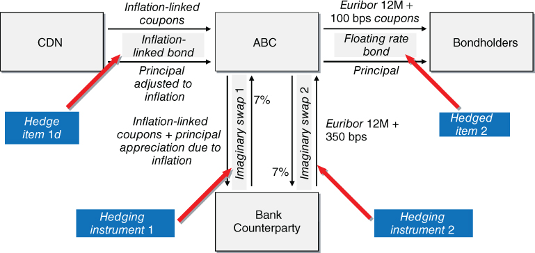
Figure 12.14 Alternative 1 – simultaneous cash flow hedging.
In a first imaginary swap, ABC would pay CDN's inflation-linked coupons and the appreciation of the principal due to inflation, and receive a fixed rate on a notional of EUR 100 million. The fixed rate would be calculated to result in a zero fair value. Suppose that the calculated fixed rate was 7%. This swap would be designated as the hedging instrument in a cash flow hedge of the purchased inflation-linked bond, with the aim of mitigating the inflation risk exposure stemming from the bond's cash flows.
In a second imaginary swap, ABC would pay 7% and receive Euribor 12-month plus 250 bps on a notional of EUR 100 million. The initial fair value of this swap should be zero. This swap would be designated as the hedging instrument in a cash flow hedge of the issued floating rate bond, with the aim of mitigating the Euribor 12-month risk exposure stemming from the bond's cash flows.
Now suppose that it designated the swap in its entirety as a fair value hedge of the inflation-linked bond (see Figure 12.15). The hedged item would be the cash flows pertaining to that bond, excluding credit risk. In my view this alternative is preferable as it is operationally simpler than the previous one, in which ABC would need to keep track of two hedging relationships, with their related documentations, effectiveness assessments, fair valuations and accounting entries.

Figure 12.15 Alternative 2 – fair value hedging of the inflation-linked swap.
Another key element to be taken into account is the greater flexibility provided by this alternative. Imagine that the CDN inflation-linked bond experienced a strong rally following a better than expected settlement of the suit, ABC could just sell the bond and unwind the swap, recognising in profit or loss the related overall gain. Under the first alternative, ABC would do the same but it would need to reclassify the amounts recognised under the second hedging relationship (the cash flow hedge of the liability) as their coupons impact profit or loss, an additional operational burden.