Now, we will experiment by adding two additional recurrent layers to the current network. The code that's incorporating this change is as follows:

# Model architecture
model <- keras_model_sequential() %>% 
         layer_embedding(input_dim = 500, output_dim = 32) %>% 
         layer_simple_rnn(units = 32, 
                          return_sequences = TRUE, 
                          activation = 'relu') %>% 
         layer_simple_rnn(units = 32, 
                          return_sequences = TRUE, 
                          activation = 'relu') %>% 
         layer_simple_rnn(units = 32, 
                          activation = 'relu') %>%
         layer_dense(units = 1, activation = "sigmoid")

# Compile model
model %>% compile(optimizer = "rmsprop",
 loss = "binary_crossentropy",
 metrics = c("acc"))

# Fit model
model_four <- model %>% fit(train_x, train_y,
0 epochs = 10,
 batch_size = 128,
 validation_split = 0.2)

When we add these additional recurrent layers, we also set return_sequences to TRUE. We keep everything else the same and compile/fit the model. The plot for the loss and accuracy values based on the training and validation data is as follows: 

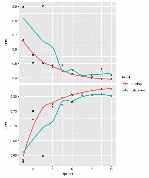
From the preceding plot, we can observe the following:

• After 10 epochs, the loss and accuracy values for training and validation show a reasonable level of closeness, indicating the absence of overfitting.
• The loss and accuracy based on the test data we calculated show a decent improvement in the results with 0.403 and 0.816, respectively.
• This shows that deeper recurrent layers did help capture sequences of words in the movie reviews in a much better way. This, in turn, enabled improved classification of the sentiment in movie reviews as positive or negative.