10
Cloud-IoT Secured Prediction System for Processing and Analysis of Healthcare Data Using Machine Learning Techniques
Department of Information Technology, Kongu Engineering College, Perundurai, Erode, Tamilnadu, India
Abstract
Data analysis converts raw data into information useful for decision-making. In recent years, the most promising research area is healthcare data analysis. For efficient analysis of data, the critical tool emerged is machine learning (ML) that uses various statistical techniques and algorithms like supervised, unsupervised, and reinforcement to predict the results of data analysis on healthcare data more precisely. In ML, various algorithms, such as supervised learning, unsupervised learning, and reinforcement learning algorithms, are used for analysis. For analyzing different healthcare data, the chapter describes varied categories of ML techniques and commonly used probability distributions in Data Science like Bernoulli, Uniform, Binomial, and Normal (Gaussian) Distribution. In the healthcare field, cloud technology and Internet of Things (IoT) offer several opportunities to clinical IT. It improves healthcare services by identifying the disease caused by the human body and contributing its non-stop methodical innovation in a massive information domain. To manipulate patient records in cloud-IoT environments is still a big challenge because of extensive data. A new model does not require the intervention of human to analyze large volume of data received from numerous origins and also sensor data is presented. Fuzzy temporal neural classifier is applied in the cloud-IoT environment to optimize the secured storage and easy handling of a vast amount of patient records. Presented work pursuits the healthcare system’s performance in reducing the execution time of patient’s request, optimizing desired garage of patient’s massive facts, and imparting records retrieval process for those applications. The experimental analysis outcome of the presented method performs better than existing benchmark systems considering parameters like disease prediction accuracy, sensitivity, specificity, F-measure, and computational time.
Keywords: Fuzzy neural classifier, disease prediction and accuracy, probability distribution, data analysis
10.1 Introduction
Healthcare is regard as a significant determinant in supporting the universal physical and mental health and comfort of people around the world. So, handling a large amount of patient’s health data in manual and electronic form is essential and challenging. An Electronic Health Record (EHR) contains a patient’s paper chart in a digitized format. EHRs were real time, containing patient records that easily and securely make information to the authorized users. The healthcare industry is generating a large amount of data that includes information about patients and their disease diagnosis reports. As the patient’s data is large, machine learning (ML) techniques are using for implementation. The data are pre-processed and used for further analysis and prediction.
ML, a powerful transformative technology, transforms human society lifestyle. ML algorithms and techniques help in predicting the disease accurately and efficiently. ML takes part a critical position in healthcare mainly for clinical decision-making. It makes the system automatically learn and develop the programs to grow and change when exposed to the new data. The application of ML in hospitals is to analyze heterogeneous data, visualize, and predict diseases. In medical domains, to identify and diagnose diseases and predict future outcomes, ML techniques and tools are used. Learning medical data encounters several difficulties since the datasets are characterizing incompleteness, noisy data (incorrect), sparseness, and inappropriate data [1]. Since 80% of healthcare data is unstructured and consists of a multitude of patient databases, ML techniques integrated with soft computing yields performance and accuracy a better one [2].
In terms of efficiency and accuracy, Internet of Things (IoT) and cloudbased applications work better than ordinary applications. Medical, military, and banking were some of the applications based on cloud and IoT applications. Cloud-based IoT applications provide services to access patient records in remote areas. Healthcare applications collect the data timely and update medical parameters severity.
Integration of cloud technology and IoT brings an improvement over processing, achieving scalability due to distributed environment, and networking capacity provides a new space to address healthcare applications. AI (Artificial Intelligence), ANN (Artificial Neural Network), ACO (optimization algorithm, Ant Colony Optimization), etc., mine large volume of data, mine the information, and extract and perform processing of real-time data in the domain of healthcare. Cloud technology offers various services to the massive cloud users with diverse and dynamic environment.
ML algorithms in the decision-making process for handling large amounts of data play a major role. The model, such as neural network clustering method, effectively identifies the disease. In this work, a large amount of data of different types such as text, image, and audio are collected through IoT devices. Cloud storage system stores the collected data. The ML algorithm groups data into normal and abnormal.
Hospitals maintain the health record for all the patients. This information is beneficial to predict all kinds of diseases. The datasets of various diseases contain the attributes and values of the particular disease needed for the prediction. ML algorithms take place a prominent part in diagnosis and prediction. The doctors use outcome gained from this to provide better medical care and increase the patient’s satisfaction. Medical data is classified into training data and test data. The algorithm uses training data to train model, and test set to measure accuracy of the model accuracy.
The chapter flow is organized as follows: Section 10.2 summarizes review on literature and Section 10.3 summarizes three different classifications of medical data. Section 10.4 proposes the various data analysis techniques used to analyze the diversified medical data. Section 10.5 describes the ML methods used in healthcare. Section 10.6 describes the probability distribution. Section 10.7 presents the various evaluation metrics to evaluate the ML model’s performance accuracy builds to solve a problem. Section 10.8 explains the function of the proposed architecture. Section 10.9 briefs the experimental results. Section 10.10 provides conclusion.
10.2 Literature Survey
Verma and Sood [3] proposed a methodology which monitors, diagnose, and predicts the severity of the disease using cloud-integrated IoT technology. It mostly pays attention on student healthcare data. Using the standard UCI Repository, systematic health data in terms of student perspective has been generated. Various classification algorithms and sensors predict the diseases affecting the students with severity. Evaluation criteria like F-measure, specificity and sensitivity, and the prediction accuracy were calculated, but the system lacks security.
Li et al. [4] presented new energy model which analyzes video stream data in cloud- IoT domain, which is produced by vehicle cameras. Both real testbeds and simulations are performed for a specific application. The main drawback is that a large number of video streams cannot be stored in IoT devices.
Stergiou et al. [5] presented fuzzy c-means segmentation technique to predict the disease and reviewed various security issues encountered in using cloud-based IoT technologies. Also, the task of cloud computing in IoT functions is demonstrated. But, the method produces less prediction accuracy.
In the work of Avinash Golande et al. [6], the accuracy of using different techniques is compared. Training data is trained using ML algorithms like decision tree, KNN, K-means clustering, and support vector machine (SVM).
In the work of Seyedamin Pouriyeh et al. [7], the ML algorithm’s performance is studied through 10-fold cross-validation method, implemented using decision tree algorithm. This algorithm is popularly used because it is fast, easy, and straightforward to interpret. Internal nodes in a decision tree represent the dataset attributes, and branches denote the outcome of each node. The SVM model is defined as a finite-dimensional vector in which each dimension represents the features. The limitation is that the response time is more.
In the work of Sellappan Palaniappan et al. [8], ML algorithms classified as supervised and unsupervised algorithms. Naive Bayes provides a new way of understanding and processing of data. The algorithm learns by calculating the correlation between the attributes (variables) and the target. The drawback is that accuracy of prediction is less and limited data is stored.
Kumar and Gandhi [9] build up three-tier architecture which handles an enormous amount of data. Firstly, the data collection process is taken care of by Tier-1. Secondly, storing a massive volume of sensor data in cloud computing is concentrated in Tier-2. Thirdly, a model is developed that identifies the symptoms of heart diseases using ROC analysis. But, the system needs security.
Gelogo et al. [10] explained different directions of applying IoT in u-healthcare applications. For IoT-based u-healthcare service, a new framework has been introduced. The results improve the performance of the healthcare service but need continuous data for diagnosis.
Gope and Hwang [11] proposed IoT-based medical device. Tiny, lightweight sensor networks monitor patients’ health remotely. Moreover, the security need is also considered in designing the healthcare system. The drawback is that the system requires security.
Hossain and Muhammad [12] proposed a healthcare industrial IoT system for online monitoring of patient health. The system analyzes health records of patients with sensors and medical devices to adverse death circumstance. The system incorporates procedures to build security like watermarking, signal enhancements to circumvent clinical errors, and identity thefts. But, it takes more resources for the processing of data.
In IoT-based healthcare environment, risks are minimized using the Intelligent and Collaborative Security Model, proposed by Islam et al. [13]. The drawback is that the response time is very high.
To predict and diagnose the various deadly diseases, Sethukkarasi et al. [14] introduced model named Neuro-Fuzzy Temporal Knowledge Representation. But, the limitation is that accuracy and specificity is smaller than existing method.
In the work of Takayuki Katsuki et al. [15], current advances in the area of the medical field developing nowadays have been discussed. Based on patient data, ML techniques play a vital role in diagnosing diseases. Presently, all health institutions are adapting to EHRs. Health information about the patient is included in EHR. These records are useful for better results and the victory of the healthcare revolution.
Ganapathy et al. [16] proposed a classifier named Temporal Fuzzy Min-Max (TFMM). It classifies medical features for effective decision-making. Also, PSO-based rule extractor agent added which brings an improvement in accuracy of disease detection. But, security components are not included.
Mohan et al. [17] proposed Hybrid Random Forest with a Linear Model (HRFLM) that uses multiclass variables and binary classification for detecting heart disease with high prediction accuracy. But, the technique does not take into account the age factor.
10.3 Medical Data Classification
Specialized analytical technique extricates valuable information and converts into a form suitable for computation. The healthcare system generates enormous patient-related data that includes X-rays, diagnostic reports, signals like ECG, laboratory records, and MRI in either documents or Electronic Medical Records (EMR). These data are classified as structured data, unstructured data, and semi-structured data [18].
10.3.1 Structured Data
It is stored in relational database. Structured healthcare data include lab test results, a hierarchy of different kinds of diseases and their symptoms, information about a diagnosis, and patient medication prescriptions such as admission history and drug.
10.3.2 Semi-Structured Data
Data that do not meet the formal structure has been stored by selfdescribing identity. It consists of data generated from sensors and is intentionally provides as a source for monitoring the behavior of patient.
10.4 Data Analysis
Structured and unstructured medical datasets have unexplored, plenty of information that can be exploited using AI methods to diagnose diseases. ML techniques provide a pathway for the professionals of healthcare to analyze such data for irregularities [20]. The regimen of health analytics currently takes a path toward sophisticated level of prescriptive analysis instead of simple descriptive level analysis. Analytics in healthcare domain apply mathematical tools which analyze a large data volume to make decisions that help improve care for every patient. The need of data analytics will improve the quality of healthcare by providing efficient medicine that reduces readmission rate, earlier detection of diseases to avoid spreading and improving treatment methods. A healthcare organization incorporates descriptive and diagnostic analytics to improve the quality of treatment. But, for tangible benefits, predictive and prescriptive health analytics can be followed [21].
10.4.1 Descriptive Analysis
Descriptive analytics are used to quantify events and generate reports. Descriptive analytics is often utilized and effectively acknowledged a variety of analytics. Descriptive health analytics has been applied to medical data in many healthcare organizations. Healthcare analytics begins with descriptive analytics that considers events occurred, consumed resources, or patient’s diagnosis charts. It helps to categorize, cluster, and classify the data, converting it into meaningful information that can enhance continuous monitoring and improve performance. Data summarization might be in the form of graphs and reports that illustrate how many patients were hospitalized, who are high-risk patients and should be treated first, the performance of surgeon, cost and facilities, etc. More number of envisioning is used by descriptive analytics [22].
10.4.2 Diagnostic Analysis
Diagnostic analytics takes the perception from descriptive analytics and dig into data, to understand the causes of those outcomes. Diagnostic analytics works on the investigation of historical data and discovers why it happens. For example, why the patient went to the hospital, and why he dropped the treatment. Diagnostic analytics needs more investigations and analysis of the health data to identify the problem cause and helps to understand the consequence faced due to that problem. In healthcare, diagnostic analytics will explore the data and make correlations [23].
10.4.3 Predictive Analysis
Predictive analytics uses historical data to train models and makes predictions on future outcomes. It tells what is likely to happen. Predictive analytics could be the advanced style of analytics and increases the accuracy of diagnosis. Predictive analytics will find the hidden patterns from large quantities of data, group the data into well-organized sets to predict the behavior, and discover the changes [24]. Predictive analytics in healthcare will accurately assess the early diagnosis of disease, risk scores for each patient by determining patterns, etc. Predictive analytics will help the health professionals by answering questions like which drugs should be used for treatment, who is likely to get the same symptoms, which patient will have the highest risk of hospitalization, and identify which patients may need additional attention [25].
10.4.4 Prescriptive Analysis
Prescriptive analytics integrates insight from all previous analyses leading to optimized decision-making. It determines what action to be taken in the future for the current problem or decision. The need for prescriptive analytics comes into picture when health problems involve too many choices to consider descriptive or predictive effectively. Prescriptive analytics identifies the problem. Prescriptive analytics predicts not only what will happen but also why it happens. For example, one can determine the drug dosage to achieve maximal cure in treatment. Alternatively, surgical choices are taken by considering the advantages and disadvantages of the surgical output. Prescriptive analytics supports both personalized medication and evidence-based medication area [26].
10.5 ML Methods Used in Healthcare
ML tools and methodology help in predicting as well as diagnosing diseases at early stages. The types of learning in ML can be classified into supervised, semi-supervised, and unsupervised learning.
10.5.1 Supervised Learning Technique
Supervised or prediction technique maps the available set of input data to a different labeled output. Build a model that can make predictions based on the relationship, which has been learned from past datasets [27]. It requires a training dataset with labels and trains the model to generate predictions for new data. If the output variable is categorical/discrete from a finite set, then the problem is called classification or pattern recognition. Predicting one of two classes, then it is a binary classification—for example: disease prediction of a patient. Suppose prediction is for more than two types, then multi-class classification [28]. The classification method helps in solving real-world problems. Supervised learning algorithms used in medical care detects lung diseases [29] and identifies different body parts from medical images [30]. It is used to predict a benign or malignant tumor to distinguish between healthy and non-healthy images in the future. It is also used to foretell the chance of heart attack within a year by analyzing earlier patients’ data. Regression is like classification used to classify if the output is a continuous value. Logistic regression predicts the patient is affected by the diseases or not because of environmental factors. Regression technique foretells patient’s life expectation [31].
ML methodologies naive Bayes classifier, C4.5 decision tree, ANNs, random forest, gradient boosted classification tree, etc., have been found to provide a different accuracy rate in disease prediction. A SVM is used to predict dementia, and its performance can be validated by statistical analysis. A supported vector machine can be used to identify rheumatoid arthritis with the patient’s prescription records and improves the accuracy of predictive models of disease [32].
Decision trees identify the unhealthy condition of patient from healthcare data [33]. Risk level prediction during pregnancy and identification of the cardiovascular problem can be performed through decision trees. The selection of feature subset in the Bayesian classifier is used to predict the survival of cirrhotic patients [34].
10.5.2 Unsupervised Learning
Unsupervised or descriptive learning finds hidden pattern. Unsupervised algorithms do not have output categories or labels on the data. Clustering is the standard unsupervised learning method for grouping data on similarity or dissimilarity measures. Phenotyping algorithms can be implemented on EMR data to identify the disease status of a group of patients who have a common diagnosis. Unsupervised learning method in healthcare includes detecting heart diseases by identifying carotid plaques and predicting hepatitis disease [35, 36]. K-means clustering algorithm predicts illness by identifying similarities in the attributes forming clusters [37]. It is used to distinguish different types of patients having more probability of being readmitted [38].
10.5.3 Semi-Supervised Learning
It learns from labeled and unlabeled data. In addition to labeled training images, it is applied for medical image segmentation [39]. A semisupervised learning technique is used to patient’s EHR for phenotype extraction [40].
10.5.4 Reinforcement Learning
Reinforcement learning learns from the opinion gathered through environment interaction and generates evaluative feedback. Feedback is provided as a reward to actions performed over time. With noisy, multi-dimensional, and incomplete data, RL provides solutions to optimal decision-making in various healthcare domains. RL approach advances toward some healthcare domains like dynamic treatment policies in chronic disease, automated medical diagnosis, i.e., mapping patient treatment history and symptoms to accurate classification of disease and other general domains like drug discovery and development, health management, etc. [41].
10.6 Probability Distributions
The two categories of probability distribution are discrete and continuous. Random variable is one which is obtained from statistical experiment outcome. Discrete random variable represents a finite set of positive integers, whereas continuous specifies infinite range values. It deals with a discrete random variable, whereas continuous probability distribution deals with a continuous random variable [42–44].
10.6.1 Discrete Probability Distributions
- – Binary Random Variable: x is either 0 or 1.
- – Continuous Random Variable: x ranges over 1, 2, 3 till m, where “m” is the total count of unique outcomes.
Each outcome of the discrete random variable contains probability. Discrete probability constitutes the association between outcome and probability. Probability Mass Function (PMF) specifies the probability of an inevitable outcome. Cumulative Distribution Function (CDF) returns probability value equal to else a value lower than a specified outcome. Percent-Point Function (PPF) provides discrete value, and the value is equal to otherwise less than given probability [42–44].
10.6.1.1 Bernoulli Distribution
The two outcomes are 0 or 1. It has only one trial. The random variable “X” takes a numeric input “one” for success probability (say, t), and input “zero” for failure (say 1 – t). Equation (10.1) shows the PMF of a Bernoulli distribution [42–44].

E(X) and V(X), expected and variance of “X”, are defined in Equations (10.2) and (10.3), respectively.
10.6.1.2 Uniform Distribution
In uniform distribution, infinite outcomes are possible [42–44]. Each outcome holds an identical probability. “X” follows uniform distribution if PDF is as shown in Equation (10.4):
E(X) and V(X), mean and variance of “X”, are defined in Equations (10.5) and (10.6), respectively.
10.6.1.3 Binomial Distribution
The binomial distribution is a distribution with only two possible outcomes 0 or 1, where probability, success (p), and failure (q) are identical on all trials, and the outcomes need not be equally likely. Events whose outcome is binary use the binomial distribution [42–44].
Equation (10.7) shows the mathematical representation for a binomial distribution.
The mean (μ) and variance Var(X) are shown in Equations (10.8) and (10.9), respectively.
If the success (p) and the count of trials (n) are known, then the formula for calculating success probability (x) among n trials is shown in Equation (10.10).
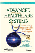
10.6.1.4 Normal Distribution
PDF defined on “X” for a normal distribution is shown in Equation (10.11).
E(X) and Var(X), mean and variance of “X”, are shown in Equations (10.12) and (10.13), respectively.
Value of mean is zero and standard deviation is one [42–44]. For such a case, PDF becomes as shown in Equation (10.14).
10.6.1.5 Poisson Distribution
Events occur in time and space of random nature [42–44]. The PMF of “X” occurring distribution that is Poisson is outlined in Equation (10.15).
Mean (μ) is defined as shown in Equation (10.16).
where
λ represents the rate at which an event occurs;
t represents the length of a time interval;
X represents the number of events in the time interval “t”.
E(X) and Var(X) are shown in Equations (10.17) and (10.18), respectively.
10.6.1.6 Exponential Distribution
Variable “X” having exponential distribution models the time occurrences among different events. Equation (10.19) shows the PDF of an exponential distribution [42–44].
λ > 0 represents the rate parameter. E(X) and Var(X), mean and variance of “X” following exponential distribution, are shown in Equations (10.20) and (10.21), respectively.
10.7 Evaluation Metrics
To build an effective ML model, evaluating a model is essential. To focus on estimating the generalization accuracy of new and unseen data, assessing a ML model is critical. The evaluation model helps in model creation and selection that provides greater accuracy in unseen data. Evaluation metrics quantify the performance of a model. Different metrics that are available evaluates the model accuracy. Some of them are listed below [45–47].
10.7.1 Classification Accuracy
It is termed as ratio of correct and input sample predictions (the total input samples in the test set) [45–47]. Classification accuracy measures how often the classifier carries out the correct predictions, which is defined as shown in Equation (10.22).
10.7.2 Confusion Matrix
A confusion matrix specifies the model performance. It depicts the detailed estimation of correct and incorrect predictions for each class. Its size is an N*N. In confusion matrix, “N” specifies number of predicted classes [45–47]. The binary classification problem consists of two classes, YES or NO, as shown in Table 10.1. Terms are defined as follows:
- – Accuracy: the proportion of sum of correct predictions.
- – Positive Predictive Value or Precision: proportion of correctly recognized positive cases.
- – Negative Predictive Value: proportion of correctly recognized negative cases.
- – Sensitivity or Recall: proportion of correctly recognized actual positive cases.
- – Specificity: It is the proportion of correctly recognized actual negative cases.
True Positive (TP): Model precisely foretells positive class. That is, the predicted and actual output was YES.
Table 10.1 Confusion matrix.
| Confusion Matrix | Target | ||||
| Positive | Negative | ||||
| Model | Positive | a | b | Positive Predictive Value | a/(a + b) |
| Negative | c | d | Negative Predictive Value | d/(c + d) | |
| Sensitivity | Specificity | Accuracy = (a + d)/(a + b + c + d) | |||
| a/(a + c) | d/(b + d) | ||||
True Negative (TN): Model precisely foretells the negative class. That is, the predicted and actual output was NO.
False Positive (FP): Model precisely foretells the positive class. That is, the predicted and actual output is YES and NO, respectively.
False negative (FN): Model precisely foretells the negative class. That is, the predicted output is No, and the actual output was YES.
10.7.3 Logarithmic Loss
It suits classification for multi-class problems. To calculate Log Loss for N samples and M classes is shown in Equation (10.23).
where
yij represents that sample data i belongs to class j or not.
pij represents that the probability of sample data i belonging to class j.
Upper bound is not specified for Log Loss. Its range is [0, 8]. It leads to greater accuracy when value is nearer to 0, whereas it achieves lower accuracy if it is away from 0. Classifier achieves greater accuracy by minimizing Log Loss. Model is estimated as better one when Log Loss value is lower [45–47].
10.7.4 Receiver Operating Characteristic Curve, or ROC Curve
It is representation of a graphical plot exemplifying diagnostic ability. It exemplifies binary classification system by varying the discrimination threshold value. The curve is created by plotting sensitivity against (1-specificity) for different threshold values [45–47].
10.7.5 Area Under Curve (AUC)
Evaluating binary classification problems is done using this metric [45–47]. The critical fundamental terms are as follows:
True Positive Rate (Sensitivity): TP/(FN + TP) gives the value of TPR. TPR refers to the proportion of TP and the sum of FN and TP [Equation (10.24)].
True Negative Rate (Specificity): TN/(FP + TN) gives the value of TNR. TNR refers to the proportion of TN and the sum of FP and TN [Equation (10.25)].
False Positive Rate: The formula FP/(FP + TN) is used to find the value of FPR. FPR refers to the proportion of FP and the sum of FP and TN [Equation (10.26)].
False Positive Rate (FPR) and True Positive Rate (TPR) range is [0, 1]. AUC ranges within 0 and 1.0. AUC created by plotting FPR vs. TPR varying values in the range [0, 1].
AUC is expedient for two reasons:
Scale-invariant: AUC is scale-invariant. Instead of considering absolute values, it evaluates the prediction accuracy.
Classification-threshold–invariant: AUC is classification-threshold–invariant. Irrespective of the threshold value chosen for classification, it measures the model’s prediction quality.
10.7.6 Precision
Precision provides the proportion of TP to the sum of TP and FP predicted by the classifier, as shown in Equation (10.27).
Greater precision value represents that algorithm brings an output a substantially more relevant results compared to that of the irrelevant ones [45–47].
10.7.7 Recall
Recall provides the proportion of correct positive samples, and all relevant identified positive samples are shown in Equation (10.28).
The high recall represents that the algorithm returns the most relevant results [45–47].
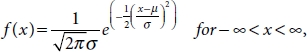
10.7.8 F1 Score
F1 score provides test’s accuracy. It ranges between [0, 1]. The best value is 1, which represents perfect precision value and recall value, and the worst is 0 specifies that how robust the classifier is. Precision represents the number of samples the classifier classifies correctly, and robust represents the classifier never omits a notable count of samples. Greater value of precision and lower recall value provides an exceedingly accurate, but the classifier omits a significant count of samples that are hard to classify. The performance of the model is better for the greater F1 score value [45–47]. Mathematically, the F1 score is defined as shown in Equation (10.29).
F1 score is an effective evaluation metric for the following classification scenarios:
- – False Positives and False Negatives are equally costly—it represents that the classifier misses on true positives or false positives.
- – Adding more data does not effectively change the effectiveness of the outcome.
- – True Negatives are high.
10.7.9 Mean Absolute Error
It defines as the average of the difference between the original and the predicted values. The measure specifies how far the predictions were away from the actual output. It does not give an idea of whether under prediction or over prediction of the data is performed [45–47]. Mathematically, it is defined as shown in Equation (10.30).
10.7.10 Mean Squared Error
Similar to Mean Absolute Error, Mean Squared Error takes the average of the square of the difference between the original and the predicted values, as shown in Equation (10.31).
Advantage of MSE:
- – It is easier to compute the gradient.
- – Effect of larger errors becomes more pronounced then smaller errors.
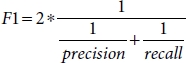
10.7.11 Root Mean Squared Error
For solving regression problems, Root Mean Squared Error (RMSE) is a widely used metric. The assumption that is followed is that the error is unbiased and normal distribution is performed [45–47]. The important points are as follows:
- – The power of “square root” provides a large number of deviations.
- – The “squared” outcome of this metric provides more robust results. It prevents neglecting of the positive and negative error values and displays the plausible error term magnitude.
- – Use of absolute error values is avoided
- – Reconstructing the error distribution using RMSE is more reliable for a large number of samples.
- – RMSE is highly affected by outlier values. Outliers to be pulled out of the data set before using this metric.
- – Compared to mean absolute error, RMSE provides higher weightage and punishes large errors.
Mathematically, the RMSE metric is defined as shown in Equation (10.32).
10.7.12 Root Mean Squared Logarithmic Error
In Root Mean Squared Logarithmic Error (RMSLE), the log of the predictions and actual values are calculated, as shown in Equation (10.33). RMSLE is mainly used when both predicted, and true values are huge numbers, when the value of RMSE decreases, the performance of the model is improved [45–47].
RMSE and RMSLE are the same if predicted, and actual values are small. RMSE is lesser than RMSLE when predicted, or the actual value is larger. RMSE is greater than RMSLE when both predicted, and the actual value is larger.
10.7.13 R-Squared/Adjusted R-Squared
R-squared is defined as shown in Equations (10.34) and (10.35).
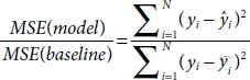
MSE(model): Mean Squared Error of the predictions opposed to the actual values.
MSE(baseline): Mean Squared Error of mean prediction opposed to the actual values.
10.7.14 Adjusted R-Squared
The formula for adjusted R-squared is as shown in Equation (10.36).
k represents the number of features.
n represents the number of samples.
When a feature is added, if R-squared value increases, the feature added brings value to the model: otherwise, the feature need not be considered [45–47].
10.8 Proposed Methodology
The Cleveland dataset is taken from the UCI repository to identify and predict the disease, and it contains 14 attributes and 304 records. The target attribute gives the result 0 or 1. If 1, then the effect is positive and indicates the presence of disease. Otherwise, it means the absence of disease.
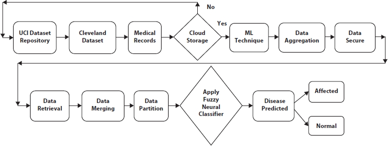
Figure 10.1 Overall classification framework.
In the proposed work, whether the person has a disease or not is predicted using one ML algorithm, fuzzy neural classifier. The proposed system is carried out into four stages, which include (1) data preprocessing, (2) cloud storage, (3) applying fuzzy neural classification algorithm, and (4) disease prediction.
Figure 10.1 illustrates that using IoT devices, details about the patient were gathered from remote areas. The UCI repository was also used for the diabetes dataset. Patient records were stored in medical records and collected from hospitals. The above process is called a data collection module. The data collection module collects the data and stores it in the cloud, and a secure storage mechanism is used to secure the data. There are five different stages in secure data mechanisms like storage, aggregation, merging, partition, and retrieval. Fuzzy neural–based classification algorithm classifies patients affected by disease and not affected by disease.
10.8.1 Neural Network
The components of neuron include inputs like hidden layer xi and output layer yi. The activation function [Equation (10.37)] like sigmoid and constant bias bc obtain the result.
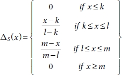
10.8.2 Triangular Membership Function
The three vertices of the triangular function ΔS(x) in a fuzzy set S are k, l, and m which are at lower, center, and upper boundaries, respectively. The membership function as shown in Equation (10.38) has lower and upper limits, which is 1, and at the centre, it is 0.
10.8.3 Data Collection
In the Cleveland dataset, a total of 303 clinical records are present, of which, six records have missing values. So, excluding it, 297 records are considered for solving a single objective fitness function. The data collected from different sources are shown in Figure 10.2.
10.8.4 Secured Data Storage
One of the popular optimization algorithms, PSO, is used to select and extract the feature with temporal constraints. Among 76 attributes of different data types with 303 patient records in the Cleveland dataset, only 13 relevant attributes are selected. The attributes used for personal identification are age and sex; it is called as primary attributes. Other remaining attributes, cp, testbps, chol, fbs, restecg, thalach, exang, olpeak, slope, ca, and thal, are called sensitive attributes as they are of high importance. “num” attribute is the target.
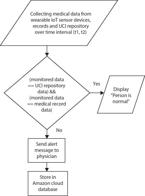
Figure 10.2 Data collection.
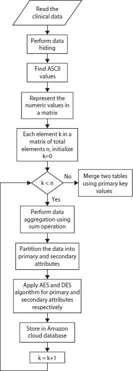
Figure 10.3 Secured data storage.
Apache HBase implemented in Hadoop Distributed File System (HDFS) accumulates massive data. As data security is the main issue in cloud storage, security algorithms such as DES and AES are used for the table of records and are depicted in Figure 10.3.
10.8.5 Data Retrieval and Merging
After retrieval of data form cloud, merging operation is performed. To restore the original values, the reverse operation of aggregation is performed as shown in Figure 10.4.
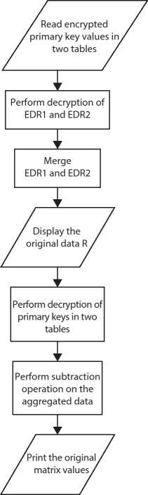
Figure 10.4 Data retrieval and merging.
10.8.6 Data Aggregation
The summation operation is used as the aggregation function to the data stored in the table after decrypting it. Then aggregation function is applied to both row and column values as indicated in Figure 10.5.
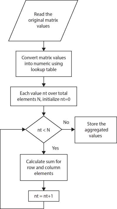
Figure 10.5 Data aggregation.
10.8.7 Data Partition
A decision tree–based split is used for partitioning the data as shown in Figure 10.6. Inputs for training samples for constructing trees are of high entropy [Equation (10.39)]. Using Divide-and-Conquer (DAC) approach in a top-down recursive manner, trees are built quickly and straightforwardly. For removing irrelevant samples on D, tree pruning is performed.
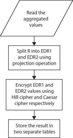
Figure 10.6 Data partition.
10.8.8 Fuzzy Rules for Prediction of Heart Disease
Rule 1:
if((age < 45)&(cp == 0)&(exang == 0)&(restecg == 0)&(slope == 1)) num = 0;
This indicates the person is normal.
Rule 2:
if((45 ≤ age < 55)&(cp == 1)&(exang == 0)&(restecg == 1)&(slope == 2)) num = 1;
This indicates the person has low severity of heart disease.
Rule 3:
if((55 ≤ age < 65)&(cp == 2)&(exang == 1)&(restecg == 1)&(slope == 2)) num = 2;
This indicates the person has moderate level of disease symptom.
Rule 4:
if((60 ≤ age < 70)&(cp == 2)&(exang == 1)&(restecg == 1)&(slope == 3)) num = 3;
This indicates the person has high level of disease symptom.
Rule 5:
if((age > 70)&(cp == 3)&(exang == 1)&(restecg == 1)&(slope == 3)) num = 4;
This indicates the person has very high level of disease symptom.
10.8.9 Fuzzy Rules for Prediction of Diabetes
if(fbs < 120)
The person does not require insulin dosage
Diabetes_symptom=type0(low):
f((120 ≤ fbs ≤ 150))
if(age < 18)
- 3–4 units of insulin dosage before pre-breakfast and pre-dinner else
- 4–5 units of insulin dosage before pre-breakfast and pre-dinner Diabetes_symptom=type1(medium):
f((150 ≤ fbs < 200)) if(age < 18)
- 5–6 units of insulin dosage before pre-breakfast and pre-dinner else
- 6–7 units of insulin dosage before pre-breakfast and pre-dinner Diabetes_symptom=type2(high):
if((200 ≤ fbs < 250))
- 7 units of insulin dosage before pre-breakfast and pre-dinner Diabetes_symptom=type2(very high):
if((250 ≤ fbs < 300))
- 8 units of insulin dosage before pre-breakfast and pre-dinner Diabetes_symptom=type2(severe):
if((fbs > 300))
9 units of insulin dosage before pre-breakfast and pre-dinner
10.8.10 Disease Prediction With Severity and Diagnosis
Training phase
For diagnosing the disease, fuzzy rules are used with Neural classifier. In training phase, most relevant features contributing to the disease are selected. Then neural tree is constructed and weights are applied to the features at Timestamp (t1,t2) for accurate decision-making as depicted in Figure 10.7.
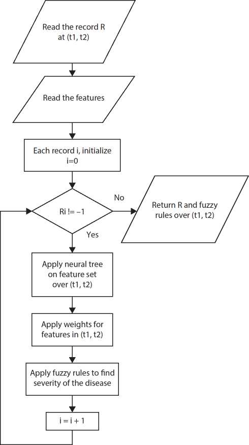
Figure 10.7 Training phase.
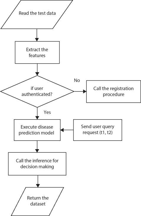
Figure 10.8 Testing phase.
Testing phase
In the testing phase, inference and expert advice are considered for decision-making as specified in Figure 10.8.
10.9 Experimental Results
The UCI repository dataset is first loaded as shown in Figure 10.9.
A security algorithm encrypts the data and stored in the cloud. Figure 10.10 lists the encrypted data.
Based on the attribute range of values, fuzzy rules are applied to find the normal and abnormal state of a person. Fuzzy temporal neural classification classifies the normal and abnormal states of a person and is shown in Figure 10.11.
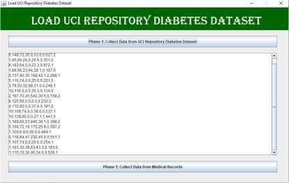
Figure 10.9 Collect data from UCI repository dataset.
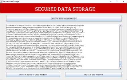
Figure 10.10 Secured data storage.
For each record, based on the class value obtained using target attribute, type of disease and its severity level is obtained and is shown in Figure 10.12.
The classification factors such as accuracy, sensitivity, specificity, precision, and F-measure are improved by using temporal attributes with fuzzy rules and providing security for cloud storage compared to existing method HRFLM, and the graphical representation is shown in Figure 10.13.
Even though additional computation is required for offering protection, decision-making is done on the right time with reduced overall computational time compared to TFMM by applying useful and smart rules, and the illustration is shown in Figure 10.14.
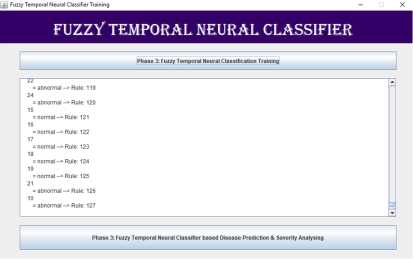
Figure 10.11 Fuzzy temporal neural classification.
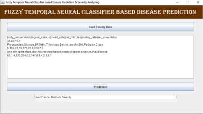
Figure 10.12 Disease prediction.
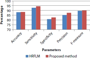
Figure 10.13 Parameters vs. percentage.
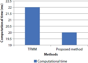
Figure 10.14 Methods vs. computational time.
10.10 Conclusion
Different forms of IoT devices such as smartphone, digital sensor, PC, laptop, and tablet are used by stakeholders to send medical requests efficiently. Cloud technology offers a reliable service in healthcare domain. The services include obtaining patent’s data, telemedicine, disease diagnosing, and storing, securing, and retrieving EMR. IoT endpoints submit massive volume of medical data in the cloud environment through internet and help to perform intelligent operations to predict valuable information from the medical data and enhance the medical services to the mankind.
Integration of cloud technology and IoT brings an improvement over processing; achieving scalability due to distributed environment, networking capacity provides a new space to address healthcare applications. ML algorithms play a significant role in predicting diseases. The proposed ML algorithm performs very well. The classification algorithms give training and testing accuracy. In the future, more experiments will be conducted to increase the performance by using other feature selection algorithms.
References
1. Magoulas, G.D. and Prentza, A., Machine Learning in Medical Applications. In: Paliouras G., Karkaletsis V., Spyropoulos C.D. (eds) Machine Learning and Its Applications, ACAI 1999, Lecture Notes in Computer Science, Springer, Berlin, Heidelberg, vol. 2049, pp 300–307, 2001. https://link.springer.com/chapter/10.1007/3-540-44673-7_19
2. Kaura, P. and Sharmab, M., MamtaMittalc, Big Data and Machine Learning Based Secure Healthcare Framework. Proc. Comput. Sci., 132, 1049–1059, 2018.
3. Verma, P. and Sood, S.K., Cloud-centric IoT based disease diagnosis healthcare framework. J. Parallel Distrib. Comput., https://doi.org/10.1016/j.jpdc.2017.11.018, 116, 27–38, 2018.
4. Li, Y., Orgerie, A.-C., Rodero, I., Amersho, B.L., Parashar, M., Menaud, J.-M., End-to-end energy models for Edge Cloud Based IoT platforms: Application to data stream analysis in IoT. Future Gener. Comput. Syst., https://doi.rg/10.1016/j.future.2017.12.048, vol. 87, 667–678, 2018.
5. Stergiou, C., Psannis, K.E., Kim, B.-G., Gupta, B., Secure integration of IoT and cloud computing. Future Gener. Comput. Syst., https://doi.org/10.1016/j.future.2016.11.031, 78, 964–975, 2018.
6. Golande, A. and Kumar, T.P., Heart Disease Prediction Using Effective Machine Learning Techniques. Int. J. Recent Technol. Eng. (IJRTE), 944–950, 2019.
7. Pouriyeh, S., Vahid, S., Sannino, G., De Pietro, G., Arabnia, H., Gutierrez, J., A comprehensive investigation and comparison of Machine Learning Techniques in the domain of heart disease. 2017 IEEE Symposium on Computers and Communications (ISCC), pp. 204–207, 2017.
8. Palaniappan, S. and Awang, R., Intelligent heart disease prediction system using data mining techniques. 2008 IEEE/ACS International Conference on Computer Systems and Applications, pp. 108–115, 2008.
9. Kumar, P.M. and Gandhi, U.D., A novel three-tier Internet of Things architecture with machine learning algorithm for early detection of heart diseases. Comput. Electr. Eng., https://doi.org/10.1016/j.compeleceng.2017.09.001, vol. 65, 222–235, 2018.
10. Gelogo, Y.E., Hwang, H.J., Kim, H., Internet of things (IoT) framework for u-healthcare system. Int. J. Smart Home, http://dx.doi.org/10.14257/ijsh.2015.9.11.31, vol. 9, 11, 323–330, 2015.
11. Gope, P. and Hwang, T., BSN-Care: A Secure IoT-Based Modern Healthcare System Using Body Sensor Network. IEEE Sens. J., 16, 5, 1368–1376, 2016.
12. Hossain, M.S. and Muhammad, G., Cloud-assisted industrial internet of things (IIoT)-enabled framework for health monitoring. Comput. Networks, https://doi.org/10.1016/j.comnet.2016.01.009, 101, 192–202, 2016.
13. Islam, S.M.R., Kwak, D., Kabir, M.H., Hossain, M., Kwak, K., The Internet of Things for Healthcare: A Comprehensive Survey. IEEE Access, 3, 678–708, 2015.
14. Sethukkarasi, R., Ganapathy, S., Yogesh, P., Kannan, A., An intelligent neuro fuzzy temporal knowledge representation model for mining temporal patterns. J. Intell. Fuzzy Syst., 10.3233/IFS-130803, 26, 3, 1167–1178, 2014.
15. Katsuki, T., Ono, M., Koseki, A., Kudo, M., Haida, K., Kuroda, J., Makino, M., Yanagiya, R., Suzuki, A., Feature Extraction from Electronic Health Records of Diabetic Nephropathy Patients with Convolutional Autoencoder. Association for the Advancement of Artificial Intelligence, 2018.
16. Ganapathy, S., Sethukkarasi, R., Yogesh, P., An intelligent temporal pattern classification system using fuzzy temporal rules and particle swarm optimization. Sadhana, https://doi.org/10.1007/s12046-014-0236-7, 39, 283–302, 2014.
17. Mohan, S., Thirumalai, C., Srivastava, G., Effective Heart Disease Prediction Using Hybrid Machine Learning Techniques. IEEE Access, 7, 81542–81554, 2019.
18. Martin-Sanchez, F. and Verspoor, K., Big data in medicine is driving big changes. Article Yearb. Med. Inform., 9, 1, 14–20, 2014.
19. Shailaja, K., Seetharamulu, B., Jabbar, M.A., Machine Learning in Healthcare: A Review. Second International Conference on Electronics, Communication and Aerospace Technology (ICECA), 2018.
20. Dash, S., Shakyawar, S.K., Sharma, M., Kaushik, S., Big data in healthcare: management, analysis and future prospects. J. Big Data, 6, Article number: 54, 1–25, 2019.
21. Groves, P., Kayyali, B., Knott, D., Van Kuiken, S., The Big Data Revolution in Healthcare: Accelerating Value and Innovation, Asia-Pacific McKinsey & Company, URI: http://hdl.handle.net/11146/465, 2013.
22. Raghupathi, W and Raghupathi, V., An Overview of Health Analytics. J. Health Med. Inform., 4, 3, 1–11, 2013.
23. Khalifa, M. and Zabani, I., Utilizing health analytics in improving the performance of healthcare services: A case study on a tertiary care hospital. J. Infection Public Health, 9, 6, 757–765, 2016.
24. Rueckel, D. and Koch, S., Application Areas of Predictive Analytics in Healthcare. Twenty-third Americas Conference on Information Systems, Boston, 2017.
25. Winters-Miner, L.A., Seven ways predictive analytics can improve healthcare, https://www.elsevier.com/connect/seven-ways-predictive-analytics-canimprove-healthcare, Elsevier, Netherlands, 2014.
26. Kuttappa, S., Optimize healthcare delivery and reduce costs with Prescriptive analytics, IBM, United States. https://www.ibmbigdatahub.com, 2020.
27. Sidey-Gibbons, J., Sidey-Gibbons, C. Machine learning in medicine: a practical introduction. BMC Med. Res. Methodol., 19, 64, 1–18, 2019.
28. Murphy, K.P., Machine Learning: A Probabilistic Perspective, p. 3, The MIT Press, Cambridge, London, 2012.
29. Shen, W., Zhou, M., Yang, F., Yang, C., Tian, J., Multi-scale Convolutional Neural Networks for Lung Nodule Classification. International Conference on Information Processing in Medical Imaging, Springer, pp. 588–599, 2015.
30. Yan, Z., Zhan, Y., Peng, Z., Liao, S., Shinagawa, Y., Zhang, S., Metaxas, D.N., Zhou, X.S., Multi-instance deep learning: Discover discriminative local anatomies for body part recognition. IEEE Trans. Med. Imaging, 35, 5, 1332–1343, 2016.
31. Qayyum, A., Qadir, J., Bilal, M., Al-Fuqaha, A., Secure and Robust Machine Learning for Healthcare: A Survey, in IEEE Reviews in Biomedical Engineering, US, vol. 14, pp. 156–180, 2021.
32. Battineni, G., Chintalapudi, N., Amenta, F., Machine learning in medicine: Performance calculation of dementiaprediction by support vector machines (SVM). Inf. Med. Unlocked, 16, 1–8, 2019.
33. Kelarev, A.V., Stranieri, A., Yearwood, J.L., Jelinek, H.F., Empirical Study of Decision Trees and Ensemble Classifiers for Monitoring of Diabetes Patients in Pervasive Healthcare. IEEE, 441–446, 2012.
34. Blanco, R., Inza, I., Merino, M., Quiroga, J., Larranaga, P., Feature selection in Bayesian classifiers for the prognosisof survival of cirrhotic patients treated with TIPS. J. Biomed. Inf., 38, 5, 376–388, 2005.
35. Pandey, A.K., Pandey, P., Jaiswal, K.L., Sen, A.K., DataMining Clustering Techniques in the Prediction of Heart Disease using Attribute selection method, International Journal of Science, Engineering and Technology Research, (IJSETR), 2, 10, 16–17, 2013.
36. Polat, K. and Güneş, S., Prediction of hepatitis disease based on principal component analysis and artificial immune recognition system. Appl. Math. Comput., 189, 2, 1282–1291, 2007.
37. Paul, R., Sayed Md., A., Hoque, L., Clustering medical data to predict the likelihood of diseases. Fifth International Conference on Digital Information Management (ICDIM), IEEE Xplore, 2010.
38. Jothi, N., Rashid, N.A., Husain, W., Data Mining in Healthcare – A Review. Proc. Comput. Sci., 72, pp. 306–313, 2015.
39. Bortsova, G., Dubost, F., Hogeweg, L., Katramados, I., de Bruijne, M., Semisupervised Medical Image Segmentation via Learning Consistency Under Transformations. International Conference on Medical Image Computing and Computer-Assisted Intervention, pp. 810–818, 2019.
40. Beaulieu-Jones, B.K. and Greene, C.S., Semi-supervised learning of the electronic health record for phenotype Stratification. J. Biomed. Inf., Cornell University, 64, pp. 168–178, 2016.
41. Yu, C., Liu, J., Fellow, IEEE, Nemati, S., Reinforcement Learning in Healthcare: A Survey, arXiv:1908.08796v4 [cs.LG], 2020.
42. https://www.analyticsvidhya.com/blog/2017/09/6-probability-distributions-data-science
43. https://towardsdatascience.com/probability-distributions-in-data-science-cce6e64873a7
44. https://machinelearningmastery.com/discrete-probability-distributions-for-machine-learning/
45. https://towardsdatascience.com/metrics-to-evaluate-your-machine-learning-algorithm-f10ba6e38234
46. https://www.analyticsvidhya.com/blog/2019/08/11-important-model-evaluation-error-metrics/
47. https://heartbeat.fritz.ai/evaluation-metrics-for-machine-learning-models-d42138496366
- *Corresponding author: [email protected]
- †Corresponding author: [email protected]