CHAPTER 26
Credit Risk and Credit Derivatives
Credit risk is dispersion in financial outcomes associated with the failure or potential failure of a counterparty to fulfill its financial obligations. In contrast to equity-related risk, which tends to have somewhat symmetrical payoff distributions, credit risk generally leads to payoff distributions that are substantially skewed to the left. In other words, the upside performance of a traditional position exposed to credit risk is limited to the recovery of the original investment plus the promised yield, whereas the downside performance could lead to the loss of the entire investment.
26.1 An Overview of Credit Risk
Default risk is the risk that the issuer of a bond or the debtor on a loan will not repay the interest and principal payments of the outstanding debt in full. A debtor is deemed to be in default when it fails to make a scheduled payment on its outstanding obligations. Default risk can be complete, in that no amount of the bond or loan will be repaid, or it can be partial, in that some portion of the original debt will be recovered.
Credit risk is influenced by both macroeconomic events and company-specific events. For instance, credit risk typically increases during recessions or slowdowns in the economy. In an economic contraction, revenues and earnings decline across a broad swath of industries, reducing the interest coverage with respect to loans and outstanding bonds for many companies caught in the slowdown. Additionally, credit risk can be affected by a liquidity crisis when investors seek the haven of liquid U.S. government securities. This was demonstrated clearly in the global financial crisis of 2007 to 2009.
Idiosyncratic or company-specific events are unrelated to the business cycle and affect a single company at a time. These events could be due to a deteriorating client base, an obsolete business plan, noncompetitive products, outstanding litigation, fraud, or any other reason that shrinks the revenues, assets, and earnings of a particular company.
As a company's credit quality deteriorates, a larger credit risk premium is demanded to compensate investors for the risk of default. In fact, the non–U.S. Treasury fixed-income market is often referred to as the spread product market. This is because all other U.S.-dollar-denominated fixed-income products (e.g., bank loans, high-yield bonds, investment-grade corporate bonds, and emerging markets debt) trade at a credit spread relative to U.S. Treasury securities. Similarly, risky debt denominated in other currencies trades at a credit spread over the bonds of the dominant sovereign issuer in that currency.
26.2 Reduced-Form Modeling of Credit Risk
Credit risk emanates from the structuring of cash flows. Cash flows are promised but are backed by an uncertain ability to meet those contractual obligations. Financial institutions and investors who have substantial exposure to credit risk look for effective ways to measure and manage their credit exposures consistently and accurately. This has led to a growing body of knowledge regarding credit models. Hedge funds and other institutions that take on credit exposure to enhance the risk-return profiles of their portfolios employ these models to implement various relative value and arbitrage strategies. Credit models are also employed to price illiquid securities that do not have reliable market prices and to calculate hedge ratios.
26.2.1 Intuition of Reduced-Form Credit Risk Models
Speaking broadly, credit models can be divided into two groups: structural models and reduced-form models. Structural models, discussed in Chapter 25, explicitly take into account underlying factors that drive the default process, such as the volatility of the underlying assets and the structuring of the cash flows (i.e., debt levels). Structural models directly relate valuation of debt securities to the financial characteristics of the economic entity that has issued the credit security. These factors usually include firm-level variables, such as the debt-to-equity ratio and the volatility of asset values or cash flows. The key is that structural credit models describe credit risk in terms of the risks of the underlying assets and the financial structures that have claims to the underlying assets (i.e., degree of leverage).
Reduced-form credit models, in contrast, do not attempt to look at the structural reasons for default risk. Therefore, reduced-form credit models do not rely extensively on asset volatility or underlying structural details, such as the degree of leverage, to analyze credit risk. Instead, reduced-form credit models focus on default probabilities based on observations of market data of similar-risk securities. In other words, reduced-form approaches typically model the observed relationships among yield spreads, default rates, recovery rates, and frequencies of rating changes throughout the market. The key feature of reduced-form credit models is that credit risk is understood through analysis and observation of market data from similar credit risks rather than through the underlying structural details of the entities, such as amount of leverage.
26.2.2 Expected Loss Due to Credit Risk
In general, the expected credit loss of a credit exposure can be determined by three factors:
- Probability of default (PD), which specifies the probability that the counterparty fails to meet its obligations
- Exposure at default (EAD), which specifies the nominal value of the position that is exposed to default at the time of default
- Loss given default (LGD), which specifies the economic loss in case of default1
The converse of LGD is the economic proceeds given default—that is, the recovery rate (RR). The recovery rate is the percentage of the credit exposure that the lender ultimately receives through the bankruptcy process and all available remedies. Therefore, LGD = (1 − RR), and RR = (1 − LGD).
Given these three factors, and expressing the loss given default through the recovery rate, the expected credit loss can be expressed as follows:
The expected loss of a portfolio of credit exposures is simply the sum of the expected credit losses of the individual exposures. In addition to expected loss exposures, analysts are generally concerned with understanding the variation in potential credit losses. Note that the variation of the potential credit losses in a portfolio of credit exposures is generally less than the sum of the variations of the individual exposures due to diversification (imperfect correlation of the individual losses).
26.2.3 Two Key Characteristics of the Risk-Neutral Modeling Approach
The previous section provided a framework and terminology with which expected losses can be modeled. This section describes a risk-neutral approach to pricing a bond with credit risk. A risk-neutral approach models financial characteristics, such as asset prices, within a framework that assumes that investors are risk neutral. A risk-neutral investor is an investor that requires the same rate of return on all investments, regardless of levels and types of risk, because the investor is indifferent with regard to how much risk is borne. Economic theory associates investor risk neutrality with investors whose utility or happiness is a linear function of their wealth.
Few, if any, investors are risk neutral with regard to substantial financial decisions. Although the assumption of risk neutrality by investors is unrealistic, the power of risk-neutral modeling emanates from two key characteristics: (1) the risk-neutral modeling approach provides highly simplified and easily tractable modeling, and (2) in some cases, it can be shown that the prices generated by risk-neutral modeling must be the same as the prices in an economy where investors are risk averse.
Let's look further at each key characteristic. One reason that the risk-neutral approach is so important to finance in general and to derivative pricing in particular is that risk-neutral price modeling is greatly simplified by not having to either differentiate between systematic and idiosyncratic risks or estimate the risk premium required to bear systematic risk. The other major reason that the risk-neutral approach to asset pricing is so essential to investments is that, as mentioned in the previous paragraph, under specific conditions, the prices obtained in a risk-neutral framework can be theoretically proven to be the same as the prices that would exist in a world of risk-averse investors. When applicable, risk-neutral pricing provides extremely simplified frameworks to price assets in a risk-averse world.
26.2.4 Pricing Risky Bonds with a Risk-Neutral Approach
Consider a risky zero-coupon, one-period debt with the face value of K (i.e., promising a cash flow of K at maturity in one period). Given the expected recovery for this bond in case of default, RR, the bond has an expected payoff of K × RR in default with the probability λ (the probability of default) and, of course, a payoff of K in the absence of default with the probability of (1 − λ).
Given the bond's forecasted cash flows, the current value (time 0) of the one-period bond, B(0,1), can be expressed in a risk-neutral model as the sum of the probability-weighted and discounted cash flows, as shown in Equation 26.2:

The first line of Equation 26.2 uses λ, a probability of default, to probability-weight the cash flows associated with the two outcomes (default and no default). Careful inspection of Equation 26.2 reveals that both potential cash flows (the cash flow in the event of default and the cash flow in the absence of default) are discounted at the riskless interest rate, r. Why would risky cash flows be discounted at a riskless rate? The answer is that it is due to the assumption of risk neutrality and that it is a technique used in risk-neutral arbitrage-free modeling.
Equation 26.2 is derived under the assumption of risk neutrality: that investors do not require a premium for bearing risk. In risk-neutral modeling, every discount rate is equal to the riskless rate. In a risk-neutral model, the probability of default, λ, is known as a risk-neutral probability. A risk-neutral probability is a probability-like value that adjusts the statistical probability of default to account for risk premiums. A risk-neutral probability is equal to the statistical probability of default only when investors are risk neutral; it should not be interpreted as the probability of default that would occur if investors were risk averse. Of course, investors are not risk neutral, and they demand a premium for investing in risky investments. To account for the risk premium, risk-neutral probabilities can be used rather than statistical probabilities. Other approaches to risk adjustment include use of higher discount rates and reduction of expected cash flows (the certainty-equivalent approach).
The second line of Equation 26.2 rearranges the first line, emphasizing the view that the price of the risky bond is equal to the price of an otherwise risk-free bond [i.e., K/(1 + r)] times an adjustment factor that accounts for the probability of default and expected recovery, or (RR × λ + [1 − λ]). Clearly, the price of the risky debt declines as the probability of default, λ, increases or the expected recovery rate, RR, declines. Risk-neutral models use a value of λ greater than the true default probability in order to reduce the values of risky cash flows relative to safe cash flows.
26.2.5 Credit Spreads
In bond markets, a bond price is often described as being determined by its credit spread, s. Equation 26.3 expresses the current price (time zero) of this debt due in one year, B(0,1), using a credit spread:
In Equation 26.3, the risk premium required to hold a risky bond is expressed through the use of a higher discount rate: the addition of the credit spread, s, to the riskless rate, r.
Equations 26.2 and 26.3 express two approaches to pricing a risky bond. Equation 26.2 calculates the price of the risky bond by adjusting its default probability (and its expected payoff), whereas Equation 26.3 obtains the price by increasing the discount rate. If done properly, both should give the same price. By setting the two equations equal to each other, the risk-neutral default probability can be related to the credit spread, as is precisely shown in Equation 26.4 and simplified into an approximation in Equation 26.5:
Equation 26.5 is an important and useful approximation. If the short-term rate and the spread are not very large, then the well-known result displayed in Equation 26.5 approximately holds. That is, the risk-neutral probability of default is equal to the credit spread divided by the expected loss given default, or (1 − RR). In the simple case of a risk-neutral world and a bond with no recovery (RR = 0), the credit spread of a bond will equal its annual probability of default!
Equation 26.6 factors the approximation in Equation 26.5 to express the credit spread as depending on the probability of default and the recovery rate:
There is substantial logic and intuition to Equation 26.6. It indicates that s, the credit spread (the excess of a risky bond's yield above the riskless yield), is equal to the expected percentage loss of the one-year bond over the remaining year under the assumption of risk neutrality. The expected annual loss is the product of the risk-neutral probability of default (λ) and the proportion of loss given default (1 − RR).
This result makes perfect sense. In a risk-neutral world, bondholders demand a yield premium on a risky bond (i.e., a spread) that compensates them for the expected losses on the bond due to default. For example, if bonds of a particular rating class tend to default at a rate of 1% per year, and if 55% of the typical bond's nominal value can eventually be recovered, then a portfolio of such bonds tends to lose 0.45% per year due to default. A risk-neutral investor would therefore require that such bonds offer a yield that is at least 0.45% higher (approximately) than the riskless bond yield to offset these expected losses.
26.2.6 Applying the Reduced-Form Models Using Risk Neutrality
Equation 26.4 should not be interpreted as predicting an actual probability of default (i.e., a true statistical probability that would exist in an economy in which investors require a premium for bearing risk). Rather, λ should be viewed as a modeling tool. The actual probability of default will be less than λ to the extent that investors demand a risk premium.
Nevertheless, the risk-neutral probability of default (λ) provides a valuable pricing tool. Risk-neutral modeling and risk-neutral probabilities can have tremendous value. The risk-neutral probability implied by one bond, presumably a highly liquid publicly traded bond, can be used as a tool for pricing other bonds. The reduced-form credit model approach utilizes riskless interest rates as discount rates much like arbitrage-free option pricing models use riskless rates rather than discount rates that contain a risk premium. That is the essence of the reduced-form modeling approach.
Consider an example in which a bond that trades in a highly efficient and liquid market has a 1% credit spread (s) and an estimated 80% recovery rate. The risk-neutral default probability of 4.7% is found using Equation 26.4) or 5% using the approximation formula in Equation 26.5).
The reduced-form approach generally uses pricing information obtained from more liquid segments of the market to price bonds that are less liquid. In other words, information implicit in bond prices that are observed in highly competitive markets is used to calibrate a model that is then used to price bonds that are less liquid. To calibrate a model means to establish values for the key parameters in a model, such as a default probability or an asset volatility, typically using an analysis of market prices of highly liquid assets. For example, the volatility of short-term interest rates might be calibrated in a model by using the implied volatility of highly liquid options on short-term bonds.
A key application of the reduced-form model is to price alternative debt securities in the same structure, such as both senior and junior debt. Note that debt securities within the same capital structure have the same underlying assets and the same probabilities of default (either the corporation defaults or it does not). The primary difference is simply the recovery rates. Senior debt should generally be expected to have higher recovery rates than junior debt, since senior debt generally has higher priority for liquidating cash flows in the bankruptcy process. Reduced-form models relate credit spreads to recovery rates, and therefore reduced-form models can be used to determine relative prices of securities in the same structure that differ in seniority.
Reduced-form models are also used to price illiquid securities based on information from liquid securities with different issuers. The credit spreads observed in competitively traded debt markets can be used to calibrate a reduced-form model and generate relatively reliable estimates of risk-neutral default probabilities. The estimated risk-neutral default probabilities can then be used to determine appropriate credit spreads for bonds of similar total risk that are not frequently traded.
The examples of the previous sections discussed single-period models with simple zero-coupon bonds. In reality, a fixed-income debt instrument represents a basket of risks: the risk from changes in the term structure of interest rates that differ in size and shape; the risk that the issuer will prepay the debt issue (call risk); liquidity risks; and the risk of defaults, downgrades, and widening credit spreads (credit risk). Sophisticated reduced-form models use the prices and, in some cases, the volatilities of riskless bonds to incorporate their effects on the prices of risky bonds.
26.2.7 Advantages and Disadvantages of Reduced-Form Models
Reduced-form models have two advantages:
- They can be calibrated using derivatives such as credit default swap spreads, which are highly liquid. (Credit default swaps are discussed later in the chapter.)
- They are extremely tractable and are well suited for pricing derivatives and portfolio products. The models can rapidly incorporate credit rating changes and can be used in the absence of balance sheet information (e.g., for sovereign issuers).
Reduced-form models have four disadvantages:
- There may be limited reliable market data with which to calibrate a model.
- They can be sensitive to assumptions, particularly those regarding the recovery rate.
- Information on actual historical default rates can be problematic. That is, few observations are available for defaults by major firms or sovereign states.
- Historical default rates on classes of borrowers (e.g., borrowers of a particular ratings class) may have limited value in the prediction of future default rates to the extent that economies undergo major fundamental changes.
Finally, it should be noted that hazard rate is a term often used in the context of reduced-form models to denote the default rate. The number is usually annualized and may be based on historical analysis of similar bonds or on expectations. Thus, an asset with a hazard rate of 2% is believed to have a 2% actual (i.e., statistical rather than risk-neutral) probability of default on an annual basis.
26.2.8 Distinguishing between Structural and Reduced-Form Credit Models
Reduced-form credit models focus on metrics, such as yields and yield spreads. These models observe, measure, and approximate the relationship between those metrics and the characteristics of the securities being analyzed, such as differences in recovery rates. The underlying motivation is to use known information (such as yield spreads) on securities in highly liquid markets to infer corresponding information (yield spreads) for other securities, while adjusting for factors such as recovery rates.
Common inputs to reduced-form credit model approaches include bond yields, yield spreads, and bond ratings, as well as historical or anticipated recovery rates and hazard rates (i.e., default rates).
Structural credit models focus on valuing securities based on option pricing models. Structural models estimate underlying asset values, degrees of leverage, and the partitioning of the assets' cash flows to debt and equity claimants.
Common inputs to structural credit models include the value of the underlying assets and equity of a structure, the face value of the debt, and estimates of the volatility of the underlying assets or equity. Like reduced-form credit models, structural credit models use riskless rates and the time to maturity of the debt.
26.3 Credit Derivatives Markets
Derivatives are cost-effective vehicles for the transfer of risk, with values driven by an underlying asset. Credit derivatives transfer credit risk from one party to another such that both parties view themselves as having an improved position as a result of the derivative. Roughly, most credit derivative transactions transfer the risk of default from a buyer of credit protection to a seller of credit protection.
26.3.1 Three Economic Roles of Credit Derivatives
The primary way that credit derivatives contribute to the economy and its participants is by facilitating risk management in general and diversification in particular. Consider the challenge faced by a major bank that has established a long-term relationship with a traditional operating firm. The bank provides many services to its clients, including payment services and credit. If the client is very large, the credit risk exposure of the bank to the firm through its loans to the firm may become substantial relative to the size of the bank. However, the bank may wish to be the sole direct creditor of the firm for several reasons. Perhaps the bank may view meeting all of the client's loan needs as increasing the chances that the bank will remain the firm's sole supplier of other services. Alternatively, the bank may wish to avoid the potential conflicts of interest and legal complexities of making loans to a firm alongside other creditors. As the sole creditor, the bank may be better able to pursue its self-interest. Credit derivatives can provide the bank with a cost-effective solution: The bank can make large loans to the firm and transfer as much risk as the bank desires to other market participants through credit derivatives. At the same time, other banks can transfer the credit risk of their portfolios to other market participants through credit derivatives. Through this process, banks and other institutions may be able to hold relatively well-diversified portfolios of credit risks while maintaining efficient and effective relationships with key clients.
Second, credit derivatives can provide liquidity to the market in times of credit stress. The availability and use of credit derivatives has soared in recent decades, with the result that credit risk has gradually changed from an illiquid risk that was not considered suitable for trading to a risk that can be traded like other sources of risk (e.g., equity, interest rates, and currencies).
Third, highly liquid markets for credit derivatives provide ongoing and reliable price revelation. Price revelation, or price discovery, is the process of providing observable prices being used or offered by informed buyers and sellers. Prices are the mechanism through which values of resources are communicated in a large economy. Ongoing and reliable price revelation regarding the credit risk of major firms serves as a highly valuable tool for decision-making and enhances overall economic efficiency.
26.3.2 Three Groupings of Credit Derivatives
Credit derivatives can differ in many ways. Following are three major methods for grouping credit derivatives.
SINGLE-NAME VERSUS MULTINAME INSTRUMENTS: Single-name credit derivatives transfer the credit risk associated with a single entity. This is the most common type of credit derivative and can be used to build more complex credit derivatives. Most single-name credit derivatives are credit default swaps (CDSs), which are the most popular way to allow one party to buy credit protection from another party.
Multiname instruments, in contrast to single-name instruments, make payoffs that are contingent on one or more credit events (e.g., defaults) affecting two or more reference entities. Credit indices are examples of multiname credit instruments. CDSs on baskets of credit risk offer specified payouts based on specified numbers of defaults in the underlying credit risks. In the most common form of a basket CDS, a first-to-default CDS, the protection seller compensates the buyer for losses associated with the first entity in the basket to default, after which the swap terminates and provides no further protection.
UNFUNDED VERSUS FUNDED INSTRUMENTS: Unfunded credit derivatives involve exchanges of payments that are tied to a notional amount, but the notional amount does not change hands until a default occurs. An unfunded credit derivative is similar to an interest rate swap in which there is no initial cash purchase of a promise to receive principal but rather an agreement to exchange future cash flows. The most common unfunded credit derivative is the CDS. As discussed later in this chapter, unfunded instruments expose at least one party to counterparty risk. Unfunded instruments can be for a single name or for multiple names.
Funded credit derivatives require cash outlays and create exposures similar to those gained from traditional investing in corporate bonds through the cash market. Credit-linked notes, discussed later in this chapter, are a common type of funded instrument. They can be thought of as a riskless debt instrument with an embedded credit derivative.
SOVEREIGN VERSUS NONSOVEREIGN ENTITIES: The reference entities of credit derivatives can be sovereign nations or corporate entities. Credit derivatives on sovereign nations tend to be more complex because their analysis has to consider not only the possible inability of the entity to meet its obligations but also the potential unwillingness of the nation to meet its obligations. The modeling of the credit risk associated with sovereign risk involves political and macroeconomic risks that are normally not present in modeling corporate credit risk. Finally, the market for credit derivatives on sovereign nations is smaller than the market for other credit derivatives.
26.3.3 Stages of Credit Derivative Activity
Both Smithson and Mengle have observed four stages in the evolution of credit derivatives activity.2 The first, or defensive, stage, which started in the late 1980s and ended in the early 1990s, was characterized by ad hoc attempts by banks to lay off some of their credit exposures.
The second stage, which began about 1991 and lasted through the mid- to late 1990s, was the emergence of an intermediated market in which dealers applied derivatives technology to the transfer of credit risk, and investors entered the market to seek exposure to credit risk.3 An example of dealer applications of derivatives technology is the total return swap, which is detailed later in this chapter. Another innovation during this phase was the synthetic securitization structure. Synthetic securitization represents the extension of credit derivatives to structured finance products, such as CDOs, in which the CDOs take credit risks through selling CDSs rather than through purchasing bonds.
The third stage was maturing from a new product into one resembling other forms of derivatives. Major financial regulators issued guidance for the regulatory capital treatment of credit derivatives, and this guidance served to clarify the constraints under which the emerging market would operate. Further, in 1999, the International Swaps and Derivatives Association (ISDA) issued a set of standard definitions for credit derivatives to be used in connection with the ISDA master agreement, as discussed in more detail later in the chapter. Finally, dealers began warehousing risks and running hedged and diversified portfolios of credit derivatives. During this stage, the market encountered a series of challenges, ranging from credit events associated with restructuring to renegotiation of emerging market debts.
The fourth stage centered on the development of a liquid market. With new ISDA credit derivative definitions in place in 2003, dealers began to trade according to standardized practices (e.g., standard settlement dates) that went beyond those adopted for other over-the-counter (OTC) derivatives. Further, substantial index trading began in 2004 and grew rapidly, and hedge funds entered the market on a large scale as both buyers and sellers.
The development of all these activities served to increase liquidity, price discovery, and efficiency in the market. And now, in the United States and elsewhere, legislation may require some credit derivatives to be exchange traded and backed by a clearinghouse; similar changes are likely to emanate from the European Union. This could take credit derivative activity into a fifth stage, from its OTC origins to the domain of the futures and derivatives exchanges.
26.4 Credit Default Swaps
By far the most important development for credit derivatives is the credit default swap. A credit default swap (CDS) is an insurance-like bilateral contract in which the buyer pays a periodic fee (analogous to an insurance premium) to the seller in exchange for a contingent payment from the seller if a credit event occurs with respect to an underlying credit-risky asset. A CDS may be negotiated on any of a variety of credit-risky investments, primarily corporate bonds.
26.4.1 Credit Default Swaps and Total Return Swaps
There are two primary types of swaps involving credit risk. The first type, by far the more predominant, is the CDS. In a CDS, the credit protection buyer pays a periodic premium on a predetermined amount (the notional amount) in exchange for a contingent payment from the credit protection seller if a specified credit event occurs. The credit protection buyer typically uses the payment to hedge losses suffered from the specified credit event. The credit protection seller receives a periodic premium in exchange for delivering a contingent payment to the credit protection buyer if a specified credit event occurs.4
Exhibit 26.1 demonstrates a CDS. In this illustration, the credit protection buyer is assumed to hold a cash position in a credit-risky asset and is using a CDS to purchase credit protection. In Exhibit 26.1, the credit risk of the underlying risky asset is transferred from the credit protection buyer to the credit protection seller. The credit protection seller may be interested in bearing the credit risk for the potential rewards or may hedge the credit risk away, using, for example, another credit derivative. Subsequent sections discuss CDSs in detail.

Exhibit 26.1 Credit Default Swap
A variation on the CDS is a total return swap with a credit-risky reference asset. In a total return swap, the credit protection buyer, typically the owner of the credit-risky asset, passes on the total return of the asset to the credit protection seller in return for a certain payment. Thus, the credit protection buyer gives up the uncertain returns of the credit-risky asset in return for a certain payment from the credit protection seller. The credit protection seller now receives both the upside and the downside of the return associated with the credit-risky asset. The credit protection seller takes on all of the economic risk of the underlying asset, just as if that asset were on the balance sheet or in the investment portfolio. Exhibit 26.2 demonstrates this total return swap.
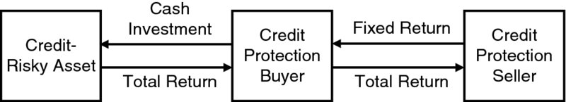
Exhibit 26.2 Total Return Swap on a Risky Asset
The left sides of both Exhibits 26.1 and 26.2 are the same and illustrate the idea that the credit protection buyer is assumed in these examples to own the underlying asset that contains the credit risk (e.g., a risky corporate bond). Comparison of the two exhibits illustrates the essential differences between a CDS and a total return swap on the same credit risk. In the case of a CDS, the credit protection buyer makes fixed payments, known as the swap premium, to the credit protection seller. If the credit experiences a trigger event (e.g., a default), the credit protection buyer receives cash from the credit protection seller. In the case of a total return swap, the credit protection buyer makes payments to the credit protection seller based on the total market return of the underlying asset. The total market return is composed of any coupon payments and any change in the underlying bond's market price. The credit protection buyer receives a payment from the credit protection seller that may vary with interest rates but does not vary based on the performance of the same credit risk.
CDSs and total return swaps on credit-risky assets are used to transfer risk. For example, a bank may use a CDS to hedge the credit exposure on its balance sheet, such as its exposure to a particular corporate borrower or to an industry that the bank believes is geared for difficult times. The bank can reduce its exposure to the credit risk of one or more of its customers, in most cases without the knowledge or consent of the customers.
CDSs are very flexible. For instance, a CDS may state in its contract the exact amount of insurance payment in the event of a credit event. Alternatively, a CDS may be structured so that the amount of the swap payment by the credit protection seller is determined after the credit event. Usually, the payment by the credit protection seller in the event of a credit event is determined by the market value of the referenced asset after the credit event has occurred. In total return swaps, there is no need to specify the events that lead to payments, since payments are driven by market values.
26.4.2 Mechanics of a Credit Default Swap
The CDS market is contract driven. This means that each CDS is a privately negotiated transaction between the credit protection buyer and the credit protection seller. Fortunately, the ISDA, the primary industry body for derivatives documentation, has established standardized terms for CDSs. These terms are not mandated for use but are available to market participants and are used as a framework for negotiating a deal. This section provides some detail regarding the standard ISDA agreement. The standard ISDA agreement serves as a template to negotiated credit agreements that contains commonly used provisions used by market participants. The standard ISDA agreement provides specifications relating to the following five aspects of the deal:
- CDS SPREAD: The CDS spread or CDS premium is paid by the credit protection buyer to the credit protection seller and is quoted in basis points per annum on the notional value of the CDS. The CDS spread is not a credit yield spread but a price or rate quote for buying credit insurance. Typically, the price of this credit insurance is paid quarterly by the protection buyer.
- CONTRACT SIZE: ISDA does not impose any limits on size or length of term of a CDS; this is up to the negotiation of the parties involved. The notional value of most CDSs falls in the range of $20 million to $200 million, with a tenor (term) of three to five years.
- TRIGGER EVENTS: This is the heart of every CDS transaction. Trigger events determine when the credit protection seller must make a payment to the credit protection buyer. Both sides to a CDS negotiate these terms intensely. The broader the definition of a trigger event, the more likely cash will flow from the protection seller to the protection buyer and the higher the appropriate spread will be. The ISDA agreement provides for seven kinds of potential trigger events; the parties to a CDS are welcome to add more, although the seven events identified by ISDA cover virtually all types of credit events:
- Bankruptcy. A filing for bankruptcy is typically associated with a company's inability to pay its debt.
- Failure to pay. Although a company may not be in bankruptcy yet, it may not be able to meet its debt obligations as they come due.
- Restructuring. This is any form of debt restructuring that is disadvantageous to a holder of the referenced credit. Restructuring is a fuzzy term, and ISDA attempts to clarify this part of the standard contract by offering the following four options for the parties to consider: no restructuring, full restructuring, modified restructuring (which limits resulting obligations to bonds maturing in less than 30 months), and modified-modified restructuring (which is less strict than modified restructuring because resulting bonds can have maturities of up to 60 months).
- Obligation acceleration. All bond and loan covenants contain provisions that accelerate the repayment of the loan or bond if the credit quality of the borrower begins to deteriorate due to a number of events, such as a failure to pay, a bankruptcy (which ISDA covers independently), or a ratings downgrade.
- Obligation default. This is any failure to meet a condition in the bond or loan covenant that would put the borrower in breach of the covenant. It could be something like the failure to maintain a sufficient current ratio or a minimum interest earnings coverage ratio.
- Repudiation/moratorium. This is most frequently associated with sovereign or emerging markets debt. It is simply a refusal by the sovereign government to repay its debt as it comes due or even an outright rejection of its debt obligations.
- Government intervention. A government's action or announcement reduces required payments or reduces the priority of making payments.
- SETTLEMENT: If a credit event occurs, settlement can be made either with a cash payment or with a physical settlement. In a cash settlement, the credit protection seller makes the credit protection buyer whole by transferring to the buyer an amount of cash based on the contract. The settlement price can sometimes be the present value of the contractual cash flows over its remaining life, or it may be determined through auction processes. Cash settlement does not occur as frequently as one might expect, because it is difficult to agree on a good market-based measure of the loss. Therefore, most CDSs use physical settlement upon the occurrence of a credit event. Under physical settlement, the credit protection seller purchases the impaired loan or bond from the credit protection buyer at par value. The credit-risky asset is physically transferred to the credit protection seller's balance sheet, and the face or par value of the bond is transferred to the protection buyer from the protection seller.
- DELIVERY: Within particular limits, the credit protection buyer has a choice of assets that can be delivered for physical settlement. This raises the issue of which of those assets is cheapest to deliver. The concept of multiple deliverable assets is common throughout derivatives and provides an option to the holder of the short option position that should be reflected in the contract's price or terms. Deliverables can include direct obligations of the referenced entity, such as corporate bonds or bank loans; obligations of a subsidiary of the referenced entity if the subsidiary is at least 50% owned by the referenced entity (sometimes referred to as qualifying affiliate guarantees); and obligations of a third party that the referenced entity may have guaranteed (known as qualifying guarantees). Note that physical settlement can create problems if there is an insufficient supply of assets to deliver, possibly because the notional value of an outstanding CDS exceeds the principal value of the underlying bonds.
Keep in mind that although ISDA provides standard terms, the parties to a CDS can negotiate any and all terms, plus add their own if they both wish. The main point is that the standardization of CDS terms has provided the infrastructure for the huge growth of the credit derivatives market.
As this example shows, four major terms define a CDS:
- CREDIT REFERENCE: CDS contracts specify a referenced asset. The referenced asset (also called the referenced bond, referenced obligation, or referenced credit) is the underling security on which the credit protection is provided. Following a credit event, particular qualifying bonds are deliverable. Typically, a senior unsecured bond is the reference entity, but bonds at other levels of the capital structure may be referenced.
- NOTIONAL AMOUNT: CDS contracts specify the amount of credit risk being transferred. This amount, agreed on by both the protection buyer and the protection seller, is analogous to the principal value of a cash bond.
- CDS SPREAD: This is the annual payment rate, quoted in basis points. Payments are paid quarterly and accrue on an actual/360-day basis. The spread is also called the fixed rate, coupon, premium, or price.
- CDS MATURITY: Typically, CDS contracts expire on the 20th of March, June, September, or December. The five-year contract is usually the most common and most liquid.
The economics of the CDS in the previous example can be viewed from the perspective of the bank. Suppose that the bank owned $20 million in face value of the referenced credit (bond). What yield would that bond be expected to offer relative to the riskless rate, given that a CDS was available at a spread of 2%? The answer is that the yield on the risky debt must exceed the yield on riskless debt of similar maturity by approximately the same rate as the CDS spread, 2%. Thus, in the example, the bank earns 2% more than the riskless rate (i.e., earns the credit spread) by holding the risky bond, then lays off all that risk by paying a 2% CDS spread. The bank as a protection buyer hedges the credit risk and earns a return equal to the riskless rate. In practice, the CDS spread can differ from the yield spread due to factors such as the counterparty risk of the CDS.
26.4.3 Valuing CDS Contracts
Generally, CDSs and other swaps are entered into without immediate cash payments from either side and are viewed as having near zero market values to each side at inception. This is because the present value of the expected premiums paid by the CDS buyer should be approximately equal to the present value of the expected payments to be made by the CDS seller. As time passes, the risk of the referenced asset may change, general credit conditions may change, and market prices and yields may change. Thus, the value of a CDS should be expected to change through time.
The process of altering the value of a CDS in the accounting and financial systems of the CDS parties is known as a mark-to-market adjustment. Investors perform a mark-to-market (MTM) adjustment to the value of CDS contracts for three primary reasons: financial reporting, realizing economic gains or losses, and managing collateral.
If the market premium moves wider than the contract premium, a protection buyer experiences an MTM gain because the protection was bought more cheaply than is currently available in the market. But if the market premium tightens, the protection seller experiences an MTM gain (and the protection buyer experiences an MTM loss). Calculating a CDS MTM adjustment is essentially the same as calculating the cost of entering into an offsetting transaction.
Suppose an investor bought five-year protection through a CDS at a spread of 100 basis points (bps) per year. One year later, the spread for the same protection (with four remaining years) has widened to 120 bps. The investor would then have an MTM gain, since the protection, for which the investor is paying 100 bps per year, now has a market value of 120 bps per year. To calculate this MTM amount, one can assume a hypothetical offsetting trade in which the investor sells identical protection at 120 bps for four years to hedge the position. This would leave a fixed residual cash flow of 20 bps per year for up to four years in favor of the investor. However, this hypothetical annuity would terminate prior to four years if a triggering credit event occurred. The present value of this annuity, adjusted for the possibility of termination prior to four years, is the MTM amount.
26.4.4 Unwinding a CDS Transaction
A party to an OTC derivative that decides to unwind a position (perhaps to monetize the gains or losses or because the credit exposure of the CDS is no longer desired) typically has three alternatives. First, the party can enter into an offsetting transaction. Second, the party can enter into a novation, also known as an assignment. A novation or an assignment is when one party to a contract reaches an agreement with a third party to take over all rights and obligations to a contract. Third, the parties to the OTC contract can agree to terminate the contract (with or without a payment from one party to the other). Details of each of these alternatives follow:
- ENTERING AN OFFSETTING POSITION: The CDS exposure can be offset with a position either in another CDS contract or in one of the underlying deliverable obligations. If the offset is in the underlying bonds, the investor has to separately hedge out the residual interest rate risk. If the offset is with another CDS contract, it most likely results in counterparty risk and a spread differential reflecting changes in the market spread since the first CDS position was established.
- ASSIGNING THE CONTRACT: Investors may be able to locate a dealer or another entity that will take over the rights and obligations of the contract with or without a cash payment from one party to the other. If so, the investor can assign (i.e., novate) the contract. The original counterparty must give permission for assignment because of the counterparty risk present in any CDS contract. The ISDA master agreement requires a transferrer to obtain prior written consent from the remaining party before a novation takes place. Due to potential exposures of CDS parties to the credit risk of the other party, assignments typically occur only when the non-dealer in the contract is replaced by a dealer.
- TERMINATING THE CONTRACT: The CDS contract can be terminated with mutual consent if necessary by having one of the counterparties pay the other counterparty any lost value from discontinuing the swap. (The valuation of an existing CDS is discussed in a previous section.)
26.4.5 Participants in Credit Derivatives Markets
Credit derivatives in general and CDSs in particular have been adopted by virtually all types of financial institutions to take on credit risk, reduce credit risk, or otherwise manage credit risk, or to implement various investment strategies. Although banks remain important players in credit derivatives markets, trends indicate that asset managers are likely to be the major force behind the future growth of these markets. Participants use CDSs for various reasons and follow different trading strategies to hedge risk, increase return, make markets, and reduce funding costs. The following are the main strategies adopted by market participants.5
- BANK TRADING ACTIVITIES: Major banks serve as market makers in credit derivatives markets and were historically constrained in their ability to provide liquidity because of limits on the amount of credit exposure they could have in one company or sector. The use of more efficient hedging strategies, including credit derivatives, has helped market makers trade more efficiently and employ less capital. Also, CDSs allow market makers to hold their inventory of bonds during a downturn in the credit cycle while remaining neutral in terms of credit risk.
- BANK LOAN PORTFOLIOS: Banks were once the primary participants in credit derivatives markets. They developed the CDS market to reduce their risk exposure to companies to which they lent money or became exposed through other transactions, thus reducing the amount of capital needed to satisfy regulatory requirements. Banks continue to use credit derivatives for hedging both single-name and broad market credit exposure.
- HEDGE FUNDS: Since their early participation in credit derivatives markets, hedge funds have continued to increase their presence and the variety of trading strategies in the markets. Whereas the activity of hedge funds was once primarily driven by convertible bond arbitrage, many funds now use CDSs as the most efficient method to buy and sell credit risk. Additionally, hedge funds have been the primary users of relative value trading opportunities and new products that facilitate the trading of credit spread volatility, correlation, and recovery rates.
- OTHER ASSET MANAGERS: Asset managers use credit derivatives markets because they provide opportunities that the managers cannot find in the bond market, such as a particular credit risk with a particular maturity. In addition, credit derivatives markets provide a relatively easy method for avoiding cash sales or overcoming difficulties of short selling. For example, an asset manager might purchase three-year protection to hedge a 10-year bond position whose creditworthiness is under stress but expected to improve if it can survive the next three years. Finally, the emergence of a liquid CDS index market has provided asset managers with a vehicle to efficiently express macro views on the credit markets.
- INSURANCE COMPANIES: The participation of insurance companies in credit derivatives markets can be separated into two distinct groups: (1) life insurers and property-casualty companies, and (2) monolines and reinsurers. Life insurers and property-casualty companies typically use CDSs to sell credit protection to enhance the return on their asset portfolios. Monolines (providers of bond guarantees) and reinsurers often sell credit protection as a source of additional premiums and to diversify their portfolios to include credit risk.
- CORPORATIONS: Operating firms use credit derivatives markets to manage credit exposure to third parties (e.g., accounts receivable). In some cases, the greater liquidity, transparency of pricing, and structural flexibility of the CDS market make it an appealing alternative to credit insurance or factoring arrangements. Some corporations invest in CDS indices and structured credit products as a way to increase expected returns on pension assets or balance sheet cash positions. Finally, corporations are focused on minimizing their funding costs; to this end, many corporate treasurers monitor their own CDS spreads as a benchmark for pricing new bank and bond deals.
26.4.6 Five Motivations for Credit Default Swaps
The following are five motivations for entering into CDSs:
- RISK DECOMPOSITION: Credit derivatives provide an efficient way to decompose and separate risks embedded in complex securities. CDS spreads reflect the price to bear pure credit risk. A corporate bond represents a bundle of risks, including interest rate risk, potential callability risk, potential currency risk, credit risk (constituting both the risk of default and the risk of volatility in credit spreads), and liquidity risk. Before the advent of CDSs, the primary way for a bond investor to adjust a credit risk position was to buy or sell that bond, consequently affecting the investor's positions across the entire bundle of risks. Credit derivatives provide a way to manage default risk independently of interest rate risks. Arbitrage strategies can be efficiently implemented using these instruments. For example, convertible arbitrage managers can use CDSs to hedge the credit risk of their convertible positions without affecting the interest rate risk of the portfolio.
- SYNTHETIC SHORTS: Credit derivatives provide an efficient way to hedge credit risk through shorting credit (i.e., taking a position with a value that varies inversely with default). The credit risk exposure of a corporate bond portfolio might be manageable by selling or shorting the bonds. However, bank loans and other credit instruments may turn out to be impossible or at least very costly to short. CDS contracts can be constructed based on those credit risks. Thus, CDSs can allow investors to establish synthetic short positions to hedge or manage specific credit risks or a broad index of credit risks.
- SYNTHETIC CASH POSITIONS: Credit derivatives offer ways to synthetically create loan or bond substitutes through tailor-made credit products. Credit derivatives are OTC instruments that can be tailored to provide investors with various choices for customizing their risk exposures. For example, investors can select maturities to express views about the timing of future credit events. CDS contracts often refer to a senior unsecured bond, but some CDS contracts refer to senior secured and syndicated secured loans. Having CDSs on several components of the same capital structure allows investors to express views on the relative values within a company's capital structure. Credit derivatives can even be used as an alternative to equity derivatives to express a directional view on a firm.
- MARKET LINKING: The high liquidity of credit derivatives can serve as a source of information that links structurally separate markets. The CDS market often reacts first and facilitates a reflection of revised prices in less liquid markets, such as bond or loan markets. For example, investors buying newly issued convertible debt are exposed to the credit risk in the bond component of the convertible instrument and may seek to hedge this risk using CDSs. As the buyers of convertible bonds purchase protection, the spreads in the CDS market widen. The spread change may occur before the pricing implications of the convertible debt are reflected in bond market spreads. However, the change in CDS spreads may cause bond spreads to widen as investors seek to maintain the value relationship between bonds and CDSs. Thus, the CDS market can serve as an information conduit and as a link between structurally separate markets.
- LIQUIDITY DURING STRESS: Credit derivatives provide liquidity in times of turbulence in the credit markets. Before the CDS market, a holder of a distressed or defaulted bond often had difficulty selling the bond, even at reduced prices, because cash bond desks are typically long credit risk due to owning an inventory of bonds. As a result, they are often unwilling to purchase bonds and assume more risk in times of market stress. In contrast, credit derivatives desks typically hold an inventory of protection (short credit risk), having bought protection through CDSs. In distressed markets, investors can reduce long credit risk positions by purchasing credit protection through credit derivatives desks, which may be better positioned to sell credit protection and change their inventory position from being short credit risk to being neutral.
26.5 Other Credit Derivatives
Generally, CDSs are not viewed as options, because in many ways they do not fit the classic view of options: They do not tend to require a single up-front premium, and they do not offer the buyer a right to initiate a transaction. However, in some ways CDSs are option-like. They tend to offer an asymmetric payout stream, much like an option: If no default or other trigger event occurs, then there is no related payment; and if there is an event, then there is a potentially large payment from the protection seller to the protection buyer. However, another key distinction between CDSs and classic options is that in most cases the decision to exercise a classic option and receive a potentially large payment is initiated at the discretion of the option buyer. In CDSs, payments are automatically triggered by specified events; there is no discretion on the part of the credit protection buyer as to whether the protection is provided or when it is provided. In summary, in credit derivatives, there can be a fine line between options and other derivatives.
The next three sections focus on credit options: credit derivatives that more closely resemble classic options. Like CDSs, credit options may be used for transferring or accumulating credit exposure. Whereas CDSs involve a series of payments from the protection buyer to the protection seller, credit options involve a single payment from the credit protection buyer to the credit protection seller that leads to an asymmetric payout (i.e., a potentially large payment from the credit protection seller to the credit protection buyer). The decision to exercise the option may be governed by the discretion of the option buyer, or it may be automatically generated by the terms of the contract and the specification of a trigger event. Thus, not all credit options give an option buyer the right but not an obligation to exercise the option.
26.5.1 Terminology of Credit Options
A credit call option allows the holder to “buy” a credit-risky price or rate, whereas a credit put option allows the holder to “sell” a credit-risky price or rate. “Buy” and “sell” are in quotation marks here to reflect that the option may be on a rate, rather than a price, and that rates are generally not viewed as being bought or sold. Typically, the underlying asset is a credit-risky bond, and so a credit put option is the right to sell a credit-risky bond at a prespecified price. However, the underlying asset can also be a credit spread. For example, a credit call option can be the right to buy a credit spread at a prespecified level.
Since prices and spreads move inversely, a call option on a price is the opposite directional bet as a call option on a rate. Thus, while either a call or a put can reference a rate or a price, an entity wishing to purchase credit protection can establish a long position in a put option on a bond price or a call option on a credit spread. The two positions both purchase credit protection because prices and credit spreads move inversely. Credit options may trade on a stand-alone basis or may be a component of a security or a contract.
Binary options (sometimes termed digital options) offer only two possible payouts, usually zero and some other fixed value. Thus, binary options do not offer the payout structure of a classic option: limited downside risk with large upside potential. Accordingly, binary credit options offer a fixed payout if exercised or triggered; traditional options offer a payout based on prevailing market conditions, such as the difference between the market price of a credit-risky asset and the strike price of the option. In a binary option, there is little or no discretion regarding exercise of the option; the binary option's contract specifies the basis on which the final payout will or will not be made. As with other options, European credit options are credit options exercisable only at expiration, and American credit options are credit options that can be exercised prior to or at expiration.
26.5.2 Credit Put Option on a Bond Price
Consider an American credit put option on a bond that pays the holder of the option the excess, if any, of the strike price of the option over the market value of the bond. The option is typically exercised if the bond experiences a credit event, such as a default. In OTC options, the contract specifies whether the exercise of the option is triggered by specified events or by the discretion of the option buyer. This option may be described as paying:
where X is the strike price of the put option and B(t) is the market value of the bond at default.
This option may be combined with the underlying credit risk to provide a hedged position. The combination of the underlying bond and the credit put option offers full repayment of the bond's principal if no credit event occurs, and payment of the option's strike price if a credit event does occur. Note that the option is not a binary option, which pays a fixed amount when a credit event occurs.
26.5.3 Call Option on a CDS
Consider an American call option on a CDS. A long position in the option is established by paying a premium. The call option allows the holder of the call option to enter a CDS at the rate (strike) specified in the option contract. Suppose that a bank holds a credit-risky asset and seeks credit protection using a call option on a CDS on the risky asset. If the credit-worthiness of the bond issuer deteriorates or if overall credit market conditions deteriorate, the credit-risky asset's price falls and its credit spread widens. After the credit spread widens, the call option holder may choose to enter a CDS at the prespecified spread by exercising the option.
The combination of a call option on a CDS and the underlying bond offers a different payout than the combination of a CDS and the underlying bond. With the call option, the bondholder can benefit from improvements in credit; the bond price rises, and the option goes out-of-the-money. If credit conditions deteriorate, the call option can be exercised to purchase credit protection using a CDS at a prespecified rate. The combination of a credit-risky bond and a CDS is hedged such that the value is protected from loss but also prevented from benefiting if credit conditions improve. Of course, the option buyer pays a premium for this ability to benefit from bond price increases while being protected from bond price declines.
26.5.4 Credit-Linked Notes
Credit-linked notes (CLNs) are bonds issued by one entity with an embedded credit option on one or more other entities. Typically, these notes can be issued with reference to the credit risk of a single corporation or to a basket of credit risks. A CLN with an embedded credit option on Firm XYZ is not issued by Firm XYZ. The CLN is like a CDS in that it is engineered to have payoffs related to the credit risk of Firm XYZ while being legally distinct from Firm XYZ.
The holder of the CLN is paid a periodic coupon and then the par value of the note at maturity if there is no default on the underlying referenced corporation or basket of credits. However, if there is some default, downgrade, or other adverse credit event, the holder of the CLN receives a lower coupon payment or only a partial redemption of the CLN principal value. Note that the cash flows received by the holder of the CLN are not delivered by the underlying referenced corporation.
Thus, the long position in a CLN bears credit risk of the referenced entity or entities without being a direct part of any bankruptcy. By agreeing to bear some of the credit risk associated with a corporation or basket of other credits, the holder of the CLN receives a higher yield on the CLN than would be received on a riskless note. In effect, the holder of the CLN has sold some credit insurance (i.e., served as a credit protection seller) to the issuer of the note (i.e., the credit protection buyer). If a credit event occurs, the CLN holder must forgo some of the coupon or principal value to make the seller of the note whole. If there is no credit event, the holder of the CLN collects an insurance premium in the form of a higher yield.
CLNs appeal to investors who wish to take on more credit risk but are either wary of stand-alone credit derivatives such as swaps and options or limited in their ability to access credit derivatives directly. A CLN is a coupon-paying note. Unlike traditional derivatives, they are on-balance-sheet debt instruments that virtually any investor can purchase. Furthermore, they can be tailored to achieve the specific credit risk profile that the CLN holder wishes to target.
26.6 CDS Index Products
CDS indices are indices or portfolios of single-name CDSs. They are tradable products that allow investors to create long or short positions in baskets of credits and have now been developed globally under the CDX (North America and emerging markets) and iTraxx (Europe and Asia) banners. The CDX and iTraxx indices now encompass all the major corporate bond markets in the world.
CDS indices reflect the performance of a basket of assets—namely, a basket of single-name CDSs. For instance, CDX and iTraxx indices consist of 125 credit names. CDS indices have a fixed composition and fixed maturities. Equal weight is given to each underlying credit in the CDX and iTraxx portfolios. If there is a credit event in an underlying CDS, the credit is effectively removed from the indices.
As time passes, the maturity term of an index decreases, making it substantially shorter than the benchmark's term. A new series of indices is established periodically, with a new underlying portfolio and maturity date to reflect changes in the credit market and to help investors maintain a relatively constant duration, if they so choose. The latest series of the index represents the current on-the-run index. Markets have continued to trade previous series of indices, albeit with somewhat less liquidity.
The indices roll every six months. Investors who were holding an existing (i.e., on-the-run) index may decide to roll into the new index by selling the old index contract and buying the new one. The new index has a longer maturity and therefore a higher market value because the credit spread curve tends to be upward sloping. The composition of the new index is likely to be different from that of the old one. For example, some of the old credit names may have been downgraded since the first index was created.
The market for CDS indices is highly liquid, meaning that the spread on a CDS index is likely to contain a smaller liquidity premium than the premium embedded in a single-name CDS. In a rapidly changing market, the index tends to move more quickly than the underlying credits, because in buying and selling, index investors can express positive and negative views about the broader credit market in a single trade. This creates greater liquidity in the indices than with the individual credits. As a result, the basis to theoretical valuations for the indices tends to increase in magnitude in volatile markets. In addition, CDX and iTraxx products are increasingly used to hedge and manage structured credit products.
Just as in the case of a single-name CDS, the credit protection buyer of a CDS index pays a fixed premium (such as 4% per year of notional value), typically on a quarterly basis. But in the case of a CDS index, the notional value of the index is based on the combined notional values of 100 or more credit risks rather than on a single credit risk. Since the referenced asset is a portfolio of credit risks, the credit protection seller must make settlement payments for credit events on each and every credit risk in the index. Each credit event in a CDS index causes a payment and then lowers the notional value of the index.
For example, consider a CDS index on 125 investment-grade U.S. corporate bonds. Suppose that an institution with a $1 billion portfolio of such bonds wishes to temporarily hedge part ($100 million) of the portfolio's risk. The institution enters a position with $100 million of notional value in the CDS index as a credit protection buyer. The credit protection buyer pays a fixed coupon on a quarterly basis to the protection seller. Suppose that during the first year, one of the 125 bonds underlying the index defaults and there is no recovery; that is, there are no proceeds to bondholders from the liquidation of the firm. The credit protection buyer would receive $800,000 from the credit protection seller, and the notional value of the CDS index would drop by $800,000. Note that the credit protection buyer and seller do not directly gain or lose when the notional value of the CDS index falls; the size of the notional value simply serves to scale the size of future payments. The CDS index functions much like a portfolio of 125 separate single-name CDSs.
26.7 Five Key Risks of Credit Derivatives
Although credit derivatives offer investors alternative strategies to access credit-risky assets, they come with specialized risks. These risks apply both to credit options and to credit swaps.
- EXCESSIVE RISK TAKING: First, there is the risk that traders or portfolio managers may use CDSs to obtain excessive and imprudent leverage, either by design or by chance. Since these are off-balance-sheet contractual agreements, excessive credit exposures can be achieved without appearing on an investor's balance sheet (although it should be discernible elsewhere in the accounts, such as in footnotes). As with all investments, proper accounting systems and other back office operations should be utilized.
- PRICING RISK: OTC credit derivatives can involve pricing risk, including risk from valuation subjectivity. As the derivative markets have matured, the mathematical models used to price derivative contracts have become increasingly complex. These models are dependent on assumptions regarding underlying economic parameters. Consequently, the pricing of credit derivatives is sensitive to the assumptions of the models and the specification of the parameters. Accounting and control procedures can be hampered by the lack of market prices.
- LIQUIDITY RISK: Another source of risk is liquidity risk. Credit derivatives that are OTC contractual agreements between two parties can be illiquid. A party to a custom-tailored credit derivative contract may not be able to obtain the fair value of the contract in exiting the position. Further, the legal documentation associated with a CDS usually prevents one party from selling its share of the CDS without the other party's consent. For a standardized CDS, there are likely to be market makers providing liquidity.
-
COUNTERPARTY RISK: Most OTC credit derivatives contain counterparty risk. Exchange-traded derivatives are backed not only by the parties on the other side of the contracts but also by institutions, such as brokerage firms and clearinghouses.
In the case of OTC options, there is only one side of a transaction that can be at counterparty risk: the long position. The reason that the long side faces counterparty risk is that if the option writer defaults, the option becomes worthless. Note that the credit protection buyer only suffers a counterparty loss when all three of the following conditions occur: the referenced entity experiences a credit event, the counterparty to the derivative defaults, and there is insufficient collateral posted to cover the loss.
The reason that the short side does not face counterparty risk is that once the option has been purchased, there is no loss to the option writer from the buyer's insolvency. However, in the case of a swap, both sides of the derivative can face counterparty risk. After a swap is initiated, it is possible for market prices to move such that one side of the contract has a positive market value and the other side has a negative market value. The side with the positive market value clearly has counterparty risk. The side with the negative market value has counterparty risk to the extent that it is possible that the market value may become positive.
The primary counterparty risk created by a CDS is to the credit protection buyer. Losses to the credit protection buyer due to counterparty risk may be manifested in two ways. First, if there is a credit event on the underlying credit-risky asset that triggers the CDS and the credit protection seller defaults on its obligations to the credit protection buyer, then the credit protection buyer can lose the entire amount due under the CDS. However, even if a trigger event has not occurred, the true value of the CDS to the credit protection buyer varies directly with the financial health of the credit protection seller. This is because reduction in the credit-worthiness of the credit protection seller decreases the probability that the seller will be able to fulfill its commitments to the buyer that are contained in the CDS.
Note that the probability that the credit protection seller will default at the same time that the referenced asset of the CDS experiences a trigger event can be relatively high if both events are driven by the same macroeconomic factors. In other words, a major credit crisis can cause CDS trigger events at a time when both the seller experiences distress and the buyer most needs the protection. It is ironic that a credit protection buyer with a goal of reducing credit risk can introduce a new form of credit risk, known as counterparty risk, into a portfolio from the purchase of a CDS.
Prior to the financial crisis that began in 2007, counterparty risk was considered a relatively small risk in credit derivative documentation. However, counterparty risk wreaked havoc on firms when Lehman Brothers, a huge financial institution, declared bankruptcy in September 2008. Even though many participants in the market had agreements with Lehman Brothers that required Lehman to post collateral, the bankruptcy of Lehman froze much of that collateral; years later, many counterparties to Lehman were still waiting for their collateral to be released through the bankruptcy process.
- BASIS RISK: Finally, credit derivatives may be viewed as having basis risk. In this context, basis risk is risk due to imperfect correlation between the values of the CDS and the asset being hedged by the protection buyer. The protection buyer takes on basis risk to the extent that the reference entity specified in the CDS does not precisely match the asset being hedged. A bank hedging a loan, for example, might buy protection on a bond issued by the borrower instead of negotiating a more customized, and potentially less liquid, CDS linked directly to the loan. If the value of the loan and the value of the bond are not perfectly correlated, there is basis risk. Another example is a bank using a CDS with a five-year maturity to hedge a loan with four years to maturity. The reason for doing so is potentially higher liquidity in CDSs with five years to maturity. However, the protection buyer takes on basis risk to the extent that the four- and five-year loan values experience different price movements.
Review Questions
-
Why is the market for fixed-income securities other than riskless bonds often termed the spread product market?
-
What are the three factors that determine the expected credit loss of a credit exposure?
-
What is the relationship between the recovery rate and the loss given default?
-
List the two key characteristics that can make risk-neutral modeling a powerful tool for pricing financial derivatives.
-
List the four stages in the evolution of credit derivative activity.
-
What is the primary difference between a total return swap on an asset with credit risk and a CDS on that same asset?
-
List the seven kinds of potential trigger events in the standard ISDA agreement.
-
How can one party to a CDS terminate credit exposure (other than counterparty risk) to a CDS without the consent of the counterparty to the CDS?
-
If a speculator believes that the financial condition of XYZ Corporation will substantially deteriorate relative to expectations reflected in market prices, should the speculator purchase a credit call option on a spread or on a price?
-
What CDS product should an investor consider when attempting to hedge the credit risk of a very large portfolio of credit risks rather than hedge a few issues?