
Chapter 12
Quantum Antenna Arrays
Iñigo Liberal1 and Richard W. Ziolkowski2
1Department of Electrical, Electronic and Communications Engineering, Institute of Smart Cities (ISC), Public University of Navarre (UPNA), Pamplona, Spain
2Global Big Data Technologies Centre, School of Electrical and Data Engineering, University of Technology Sydney, Ultimo, New South Wales, Australia
12.1 The Rise of Quantum Technologies
Quantum technologies are defined by their ability to harness quantum mechanical effects in order to achieve performances that cannot be attained within the boundaries of classical physics. In doing so, quantum technologies hold the promise to revolutionize communication, sensing, simulation and computing technologies, thus bringing transformative advances to science, industry and society [1]. Photonic quantum technologies, for which light acts a fundamental resource, are arguably the major driving force in promoting basic quantum technologies to commercial systems. For example, quantum key distribution (QKD) is the most promising example of a commercial quantum communication system [2]. QKD enables a secure channel with the guarantee that interceptions in the communication can be detected, an invaluable property to distribute cryptographic keys. By using optical links, several companies currently offer commercial QKD systems [3–5], and satellite QKD communications have been demonstrated by state‐driven enterprises [6]. Similarly, quantum sensing takes advantage of nonclassical field correlations to enable metrology with an unprecedented precision. The use of nonclassical light at the Laser Interferometer Gravitational‐wave Observatory (LIGO) is perhaps the most iconic example of a practical quantum metrology system [7]. However, sensing via the optical readout of solid state spins have enabled a myriad of applications, fascinating examples including temperature mapping within a neuron [8], intra‐bacterial magnetic field mapping [9], nuclear magnetic resonance of single proteins [10], and nanoscale magnetic resonance imaging (MRI) [11], only to name a few. Quantum computing, while still a futuristic goal [12], is the most appealing quantum technology application for the general public. Despite the fact that many fundamental challenges must be addressed, several companies are investing in the development of a practical optical quantum computer [13, 14]. In fact, the first demonstration of quantum computation advantage was based on a photonic device [15]. These are only a few examples of how quantum photonic technologies are a growing reality that will only continue to increase its impact in the following years.
Nonclassical light states are the fundamental resource driving most of the aforementioned photonic quantum technologies. For example, single‐photon states are the basis of QKD communications systems, squeezed light states and N00N states empower sensing below shot noise, and single‐photon and cluster states give power to linear‐optics quantum computers. Therefore, the design of light sources capable of generating prescribed nonclassical light states is one of the most important aspects in developing photonic quantum technologies.
In an entirely different field, the vast body of research nowadays known simply as antenna theory has led to a high degree of sophistication in the ability to tailor the radiation characteristics of electromagnetic waves emitted by innumerable types of sources. Previous chapters of this book have focused on classical antennas and antenna arrays; they exemplify how this is indeed the case. Without any doubts, much of this work can be applied to catalyze the design of nonclassical light sources. Based on this perspective, and following the general themes of this book, we will discuss in this chapter how photon statistics can be engineered by designing the geometry of quantum antenna arrays. The main goal is to summarize the basic theory behind quantum antenna arrays, providing antenna designers with the tools to explore how their know‐how can be applied to the exciting field of quantum technologies. In doing so, we will explore intriguing nonclassical light sources with no classical counterparts, including directionally entangled photon bunches and perfectly isotropic single‐photon sources.
To achieve our goal, we will begin with an overview of quantum antenna array theory. While arrays of electrically small classical antennas were described in Chapter 10, the radiating elements herein are physically extremely small being quantum emitters, i.e. atoms. We then follow with a relevant introduction to the concepts of photon statistics, emphasizing directional correlations. These two fields are then combined to reveal how the design of linear arrays of quantum emitters can enable beamforming of their photon statistics. We emphasize the effects that can and cannot be observed in classical systems. Examples of first, second and Nth order correlation outcomes demonstrate how their directivities can be tailored by a quantum array's configuration. We apply these results to understand how one could in fact achieve an isotropic single‐photon source. We also address the difficulties associated with the very contrasting concept of quantum superdirectivity. A description of the technologies available today that are the most promising to realize these exciting quantum array results is given. Finally, we explore the many possible future directions of the field of quantum antenna arrays and the concurrent opportunities for electromagnetic scientists and engineers.
12.2 Quantum Antenna Array Theory
We start by introducing the basic quantum theory of radiation for an array of quantum emitters. We try throughout to establish the connections with classical antenna array theory that was the focus of most of the previous chapters of this book. In particular, the final expressions are written in forms that are readily connected to their classical counterparts.
12.2.1 Macroscopic Quantum Electrodynamics
As a first approach to quantum antenna arrays, we analyze the general scenario schematically depicted in Figure 10.1. An array of ![]() quantum emitters is depicted that is coupled to a macroscopic photonic environment through the fields radiated by its individual elements. This complex environment is characterized by a relative permittivity distribution,
quantum emitters is depicted that is coupled to a macroscopic photonic environment through the fields radiated by its individual elements. This complex environment is characterized by a relative permittivity distribution, ![]() . Quantum excitation in such macroscopic environment will be modeled as a bath of polaritonic modes (i.e. a polariton is a quasi‐particle formed when a photon couples strongly with an exciton, e.g. a phonon, and, hence, it represents a joint state of light and matter) following the macroscopic quantum electrodynamics (QED) formalism (see, e.g. [16–18]). This approach allows for the analysis of lossy and dispersive media. We restrict the analysis in this chapter to the case of isotropic dielectric media, which is typical of most configurations at optical frequencies. However, generalizations of the same quantization procedure to account for magnetically polarizable, bi‐anisotropic, and nonlocal media are available [19]. While most quantum optics textbooks treat the decay of quantum emitters from the Schrödinger and/or interaction pictures, here we will adopt the Heisenberg picture because fully time‐evolving field operators bring a closer analogy to classical antenna theory.
. Quantum excitation in such macroscopic environment will be modeled as a bath of polaritonic modes (i.e. a polariton is a quasi‐particle formed when a photon couples strongly with an exciton, e.g. a phonon, and, hence, it represents a joint state of light and matter) following the macroscopic quantum electrodynamics (QED) formalism (see, e.g. [16–18]). This approach allows for the analysis of lossy and dispersive media. We restrict the analysis in this chapter to the case of isotropic dielectric media, which is typical of most configurations at optical frequencies. However, generalizations of the same quantization procedure to account for magnetically polarizable, bi‐anisotropic, and nonlocal media are available [19]. While most quantum optics textbooks treat the decay of quantum emitters from the Schrödinger and/or interaction pictures, here we will adopt the Heisenberg picture because fully time‐evolving field operators bring a closer analogy to classical antenna theory.
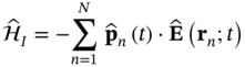
The Hamiltonian of the system depicted in Figure 12.1 is given by the addition of the Hamiltonians for the array of quantum emitter's and the electromagnetic field plus polarizable matter (i.e. the polaritonic) system, as well as the interaction Hamiltonian between both systems:
The emitters are modeled as two‐level systems ![]() that are located at positions
that are located at positions ![]() and have the transition frequency
and have the transition frequency ![]() and dipole moment
and dipole moment ![]() . This choice leads to the Hamiltonian
. This choice leads to the Hamiltonian

where ![]() is the Pauli operator with
is the Pauli operator with ![]() .
.
Excitations in the macroscopic photonic environment are modeled as a continuum of polariton modes for each position ![]() , frequency
, frequency ![]() , and polarization
, and polarization ![]() with annihilation operators
with annihilation operators ![]() . They can also be written in vector form as
. They can also be written in vector form as ![]() and obey equal‐time bosonic commutation relations:
and obey equal‐time bosonic commutation relations:
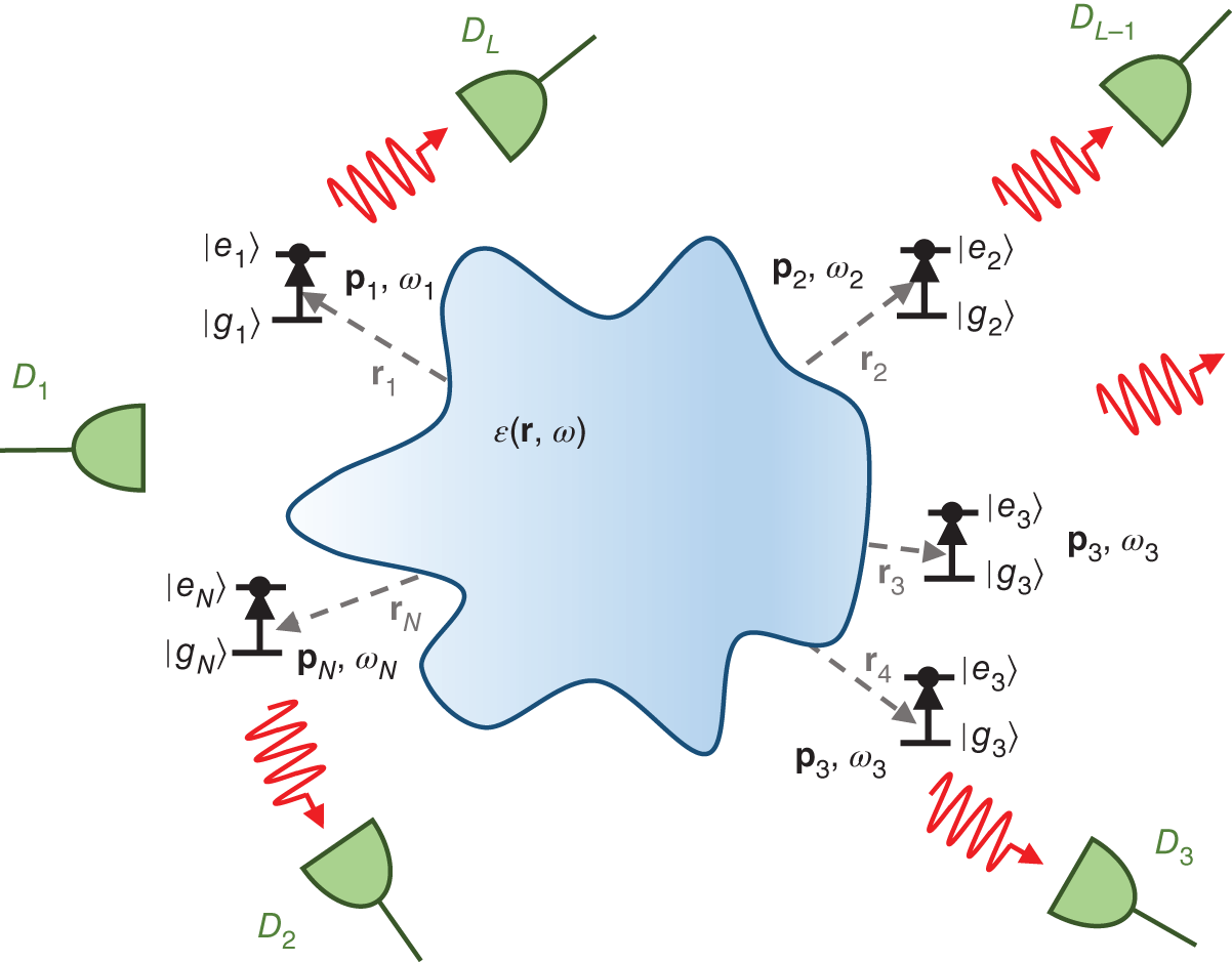
Figure 12.1 Quantum antenna arrays in a complex environment. Schematic depiction of a quantum antenna array composed of  two‐level systems
 , with transition frequencies
  and transition dipole moments
  located at positions
  and immersed in a macroscopic photonic environment characterized by a lossy and dispersive permittivity distribution
  . A set of
  detectors consisting of photon counters is situated around the array in the same environment.
In this manner, the Hamiltonian for the macroscopic photonic environment can be compactly written as

Finally, we consider an interaction Hamiltonian within the electric dipole approximation
where ![]() , with
, with ![]() and
and ![]() being the annihilation and creation operators associated with the nth emitter and with
being the annihilation and creation operators associated with the nth emitter and with ![]() . Note that because we are assuming point‐like emitters with an electric dipole transition, the electric field operator is evaluated at the position of the emitters
. Note that because we are assuming point‐like emitters with an electric dipole transition, the electric field operator is evaluated at the position of the emitters ![]() . This approximation is similar to assuming that the elements of a classical antenna array are electric Hertzian dipoles. However, similar to antenna theory, it is possible to further control the quantum radiated field by engineering the current distributions of the individual radiating emitters [20].
. This approximation is similar to assuming that the elements of a classical antenna array are electric Hertzian dipoles. However, similar to antenna theory, it is possible to further control the quantum radiated field by engineering the current distributions of the individual radiating emitters [20].
The electric field operator is given by

where we have introduced the response function

which is proportional to the classical dyadic Green's function ![]() [21]. Equation (12.6) intuitively conveys the idea that the electric field operator can be understood as the result of radiation by the polaritonic excitations in the macroscopic environment. Therefore, it is not surprising that the classical dyadic Green's functions play the role of a propagator in such a process. However, the antenna designer might be surprised that the propagation term also includes the square root of the imaginary part of the permittivity as a coupling term between fields and environmental excitations. Intuitively, it makes sense that the effective exchange of energy between fields and matter must be mediated by dissipation. From a more rigorous perspective, this term is exactly what is needed to reconstruct the macroscopic Maxwell's equations from the coupling of the free‐space fields and matter when the quantum mechanical canonical quantization of the fields is required and employed in the presence of matter [17]. The presence of the square root of the imaginary part of the permittivity also ensures that the fluctuation dissipation theorem, as it is often invoked in the semiclassical treatment of thermal emission [22], directly emerges from this framework.
[21]. Equation (12.6) intuitively conveys the idea that the electric field operator can be understood as the result of radiation by the polaritonic excitations in the macroscopic environment. Therefore, it is not surprising that the classical dyadic Green's functions play the role of a propagator in such a process. However, the antenna designer might be surprised that the propagation term also includes the square root of the imaginary part of the permittivity as a coupling term between fields and environmental excitations. Intuitively, it makes sense that the effective exchange of energy between fields and matter must be mediated by dissipation. From a more rigorous perspective, this term is exactly what is needed to reconstruct the macroscopic Maxwell's equations from the coupling of the free‐space fields and matter when the quantum mechanical canonical quantization of the fields is required and employed in the presence of matter [17]. The presence of the square root of the imaginary part of the permittivity also ensures that the fluctuation dissipation theorem, as it is often invoked in the semiclassical treatment of thermal emission [22], directly emerges from this framework.
12.2.2 The Quantum Field in the Far‐Zone
The Hamiltonian formulated in Section 12.2.1 is the standard formulation of macroscopic QED [16–18]. Next, we derive an expression for the radiated field in the far zone that has very clear analogies with antenna theory. To this end, we compute the Heisenberg equation of motion, ![]() , for the polaritonic operator
, for the polaritonic operator ![]() , and integrate it, leading to its decomposition into the free‐evolving and source parts
, and integrate it, leading to its decomposition into the free‐evolving and source parts
Physically, the free‐evolving part corresponds to the electromagnetic field and matter evolution that would be taking place in the absence of the interactions with the quantum emitters. It can be written as:
On the other hand, the source part corresponds to the excitations of the electromagnetic field and matter system induced by the interaction with the quantum emitter system. It is given by

with

By introducing (12.8) into (12.6), we find that the electric field operator can be similarly decomposed into free‐evolving and source driven parts
with

Introducing (12.11) into (12.6), using the completeness relation of the dyadic Green's function to compute the volume integral, and noting that ![]() is an odd function in
is an odd function in ![]() , the contribution of each emitter to the source field can be written as a memory kernel acting on the electric dipole operator
, the contribution of each emitter to the source field can be written as a memory kernel acting on the electric dipole operator
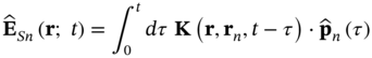
with

Recalling that the electric dipole operator is ![]() , the decomposition of the source electric field operator into positive and negative frequency components is a useful approach:
, the decomposition of the source electric field operator into positive and negative frequency components is a useful approach:
with
and
Physically, the positive frequency component is associated with the radiation of one photon by the emitter (as a transmitter), while the negative frequency component represents the absorption of one photon by the emitter (as a receiver). A very compact expression for the electric field operator can now be obtained by applying the Laplace transform to these operators:

and then evaluating the integral over all frequencies via complex analysis techniques. The result is that Eq. (12.17) can be written as
The formulation up to this point has been developed for an arbitrary photonic environment. Particular cases can be addressed by introducing a specific form of the dyadic Green's function. Thus, we assume that the emitters are immersed in free‐space and the observation point for the electric field is in the far‐zone of this system to establish a closer connection with antenna theory.
The classical dyadic Green's function for this case is

with ![]() ,
, ![]() ,
, ![]() , and the unit vector
, and the unit vector ![]() . The first‐order approximation to
. The first‐order approximation to ![]() is given by the well‐known expression:
is given by the well‐known expression: ![]() . We keep this first‐order approximation in the exponential and only the zero‐order approximation in the other terms. The dyadic Greens function then becomes
. We keep this first‐order approximation in the exponential and only the zero‐order approximation in the other terms. The dyadic Greens function then becomes
with ![]() . In this manner, we can rewrite the electric field operator as
. In this manner, we can rewrite the electric field operator as

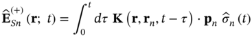
Finally, we apply the inverse Laplace transform and get the general form for the source electric field in the far zone
with ![]() being the delayed time with respect to the origin of the coordinates.
being the delayed time with respect to the origin of the coordinates.
12.2.3 Decay Dynamics in the Noninteracting Markovian Regime
Equation (12.24) describes the electric field operator in the far‐zone for an arbitrary time evolution of the quantum emitter operator. This formalism can be applied to a variety of configurations. We particularize it here to the case of the decay dynamics of noninteracting quantum emitters in the weak coupling regime. Thus, we will show that it exhibits a simple exponential decay. This case corresponds to the physical situation in which each emitter operates as an independent single‐photon source.
First, we analyze the Heisenberg equations of motion, ![]() , for the quantum emitter annihilation operator
, for the quantum emitter annihilation operator ![]() . They lead to the relation for the
. They lead to the relation for the ![]() th emitter:
th emitter:
Next, we clarify the approximations involved in assuming a simple exponential decay rate.
We begin by assuming that the macroscopic photonic environment is initially in the vacuum state. We can then substitute ![]() for all relevant interactions. From an antenna theory perspective, this condition is similar to assuming that there are no external sources to the problem. In addition, we assume that the emitters are not interacting amongst themselves. This allows us to approximate
for all relevant interactions. From an antenna theory perspective, this condition is similar to assuming that there are no external sources to the problem. In addition, we assume that the emitters are not interacting amongst themselves. This allows us to approximate ![]() . This is the typical assumption in antenna theory where each element of the array is driven independently, and the array geometry is designed so that the coupling between each of the antenna elements in the array is weak enough.
. This is the typical assumption in antenna theory where each element of the array is driven independently, and the array geometry is designed so that the coupling between each of the antenna elements in the array is weak enough.
We also introduce the low‐excitation approximation (also known as the one‐photon correlation approximation). It consists of replacing ![]() . This approximation is similar to having started with a Hamiltonian within the rotating wave approximation. For the problem of initially‐excited noninteracting quantum emitters, this means that each emitter effectively sees only a single excitation. It is a very accurate approximation.
. This approximation is similar to having started with a Hamiltonian within the rotating wave approximation. For the problem of initially‐excited noninteracting quantum emitters, this means that each emitter effectively sees only a single excitation. It is a very accurate approximation.
Even with all of these approximations, the model still is capable of describing both the weak and strong coupling regimes. These are the ones in which most optical systems operate. However, the approximation will not be valid in the ultra‐strong coupling regime where the number of excitations is not preserved.
With these approximations and the application of the Laplace transform, the equation of motion for ![]() reduces to
reduces to
Using (12.20) and rearranging its terms we find the following expression for the Laplace‐transformed emitter operator:
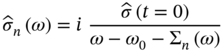
where we have introduced the emitter's self‐energy ![]() :
:

Finally, the standard Born–Markov approximation consists of neglecting the dispersion of the self‐energy, i.e. ![]() . This approximation is accurate when the coupling between the emitter and the photonic environment is small. This situation is usually referred to as the weak‐coupling regime. The approximation is also equivalent to assuming that the interaction between the emitter and the photonic environment has no memory effects.
. This approximation is accurate when the coupling between the emitter and the photonic environment is small. This situation is usually referred to as the weak‐coupling regime. The approximation is also equivalent to assuming that the interaction between the emitter and the photonic environment has no memory effects.
Within this approximation, the imaginary part of the self‐energy corresponds to the decay rate ![]() associated with the exponential decay. On the other hand, the real part of the self‐energy results in a frequency shift,
associated with the exponential decay. On the other hand, the real part of the self‐energy results in a frequency shift, ![]() .
.
Note that the real part of the dyadic Green's function diverges. As a consequence, the self‐energy must be properly renormalized to properly compute this frequency shift which is well‐known as the Lamb shift. However, since this small shift does not affect the overall decay dynamics, it is typically assumed that it was included in the transition frequency of the emitter, ![]() . Finally, within all of these approximations, we recover the usual exponential decay expression:
. Finally, within all of these approximations, we recover the usual exponential decay expression:
After detailing all of the approximations leading to the simple exponential decay, it might seem that it is a crude approximation that can only be applied in very restricted circumstances. However, the truth is that for most weekly interacting single‐photon sources, exponential decay is a very accurate approximation. On the other hand, observing non‐exponential decay dynamics is a challenging experimental task in most configurations.
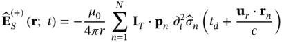
Finally, by introducing (12.29) into (12.24) we find the expression for the positive frequency electric field operator that we will use in the rest of the chapter:

The term
where

12.3 Photon Statistics
The theory detailed in Section 12.2 shows that the temporal and spatial variations of the electric field operator are the same as those of a classical field. This outcome suggests that many aspects of the theory learned for the design of classical antenna arrays could be transferred to quantum antenna arrays. At the same time, it is expected that quantum antenna arrays will give access to effects that cannot be observed in classical systems. This is indeed the case.
Quantum effects fundamentally arise in the measurement of photon statistics, i.e. in coincidence photon measurements. Early experiments in the 1970s and 1980s confirmed that the measurements of photon statistics cannot be explained by a classical theory. They revealed numerous novel phenomena including antibunching [23], two‐photon cascade emission [24] and violation of Bell's inequalities [25]. These effects provide the most direct evidence that a quantum theory of light is needed. Moreover, correlations that cannot be achieved by classical systems are the major driving force behind the currently evolving quantum technologies. Being the most direct experimental proof for quantum mechanics, early experiments have been very critically analyzed, motivating researchers to identify loopholes invalidating the conclusions extracted from them [26–28]. Nevertheless, the improved and loophole‐free experimental setups continue to confirm the quantum theory [29–31].
Following the theme of antenna arrays, we outline in this section the basic theory needed to describe how the geometry of a quantum antenna array influences directional correlations in photon statistics. To this end, we assume that the quantum antenna array is surrounded by a number ![]() of photon counters located at positions
of photon counters located at positions ![]() ,
, ![]() . We also assume that these devices operate via direct photon detection, though alternatives such as homodyne detection might be considered [32]. Therefore, the detectors can be phenomenologically modeled by using Glauber's theory of optical coherence [33, 34], which connects the probability of photon coincidence detections with field correlations.
. We also assume that these devices operate via direct photon detection, though alternatives such as homodyne detection might be considered [32]. Therefore, the detectors can be phenomenologically modeled by using Glauber's theory of optical coherence [33, 34], which connects the probability of photon coincidence detections with field correlations.
Specifically, a measurement event can be modeled as a change in the quantum state of the detector from ![]() to
to ![]() , triggered by the absorption of a photon. Since the annihilation of environmental excitations is described by the positive frequency electric field operator, the probability amplitude for a photon with polarization
, triggered by the absorption of a photon. Since the annihilation of environmental excitations is described by the positive frequency electric field operator, the probability amplitude for a photon with polarization ![]() to be detected at time
to be detected at time ![]() and location
and location ![]() is
is ![]() . Consequently, the total probability density of detecting a photon is proportional to the sum over all of the probabilities for each final state:
. Consequently, the total probability density of detecting a photon is proportional to the sum over all of the probabilities for each final state:


where we have made use of the identity operator ![]() to obtain the intermediate expression.
to obtain the intermediate expression.
For a set of ![]() detectors, the procedure outlined earlier can be generalized to describe the coincidence measurement of
detectors, the procedure outlined earlier can be generalized to describe the coincidence measurement of ![]() photons with
photons with ![]() polarizations, at different times
polarizations, at different times ![]() , and for different positions
, and for different positions ![]() :
:
If we assume that the detectors are in the far‐zone of the array at positions ![]() it is clear from Eq. (12.31) that the photon statistics are not affected by the separation distance
it is clear from Eq. (12.31) that the photon statistics are not affected by the separation distance ![]() . Therefore, it is possible to define the probability density per unit
. Therefore, it is possible to define the probability density per unit ![]() and
and ![]() as:
as:
The probability density ![]() described by Eq. (12.35) enables the study of interesting spatio‐temporal correlations. Importantly, it can be shown that any other photon statistic can be constructed from such a probability density [35, 36].
described by Eq. (12.35) enables the study of interesting spatio‐temporal correlations. Importantly, it can be shown that any other photon statistic can be constructed from such a probability density [35, 36].
As classical antenna array theory and its practical applications emphasize, directivity is a major performance characteristic associated with any array. Consequently, we are most interested in the directional correlations that can be induced by the geometry of a quantum array. In order to emphasize the directional behavior of its emissions, independent of the times at which the measurements take place, we define the time integral of the probability density:

The integrated correlations ![]() represent the average number of
represent the average number of ![]() ‐photon coincidence measurements for any time delay. They are a good figure of merit of how “bunched” the photons are in different directions after their emission.
‐photon coincidence measurements for any time delay. They are a good figure of merit of how “bunched” the photons are in different directions after their emission.
The functions (12.36) include time integrals over rapidly oscillatory functions that are related to the transition frequency of the dipoles, ![]() . Unless the transition frequencies are very close to each other, these integrals will average to zero over time. As a consequence, interference phenomena might only be observable for short time intervals. In general, this property indicates that no quantum interference of any significance will take place unless the emitters have similar transition frequencies, i.e.
. Unless the transition frequencies are very close to each other, these integrals will average to zero over time. As a consequence, interference phenomena might only be observable for short time intervals. In general, this property indicates that no quantum interference of any significance will take place unless the emitters have similar transition frequencies, i.e. ![]() . In such a case, the time‐integrated correlation (12.36) reduces to:
. In such a case, the time‐integrated correlation (12.36) reduces to:

with ![]() . With this general form, time‐integrated correlation functions of arbitrary order can be evaluated for any array geometry and initial state of the emitters in the quantum array.
. With this general form, time‐integrated correlation functions of arbitrary order can be evaluated for any array geometry and initial state of the emitters in the quantum array.
12.4 Linear Array of Quantum Emitters
We illustrate the applicability of the theory outlined earlier by studying the photon statistics of a uniform vertical linear array of quantum emitters, an archetypical geometry in textbooks of antenna theory [37–40]. Specifically, we consider the geometry schematically depicted in Figure 12.2, where all of the emitters are located at the positions ![]() along the
along the ![]() ‐axis with equal separation distance
‐axis with equal separation distance ![]() , and each has its transition dipole moment also oriented along the
, and each has its transition dipole moment also oriented along the ![]() ‐axis, i.e.
‐axis, i.e. ![]() .
.

Figure 12.2 Uniform linear vertical arrays. Schematic depiction of a uniform vertical linear array of  quantum emitters. The emitters are located at positions
  along the
  ‐axis and are separated uniformally by the distance
  . Each emitter has a transition dipole moment,
  , that is also oriented along the
  ‐axis.
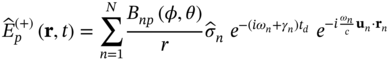
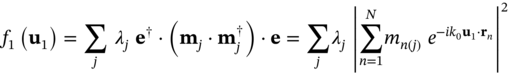
For this particular configuration, the far‐zone electric field operator has a single polarization component ![]() . Then, Eq. (12.24) reduces to
. Then, Eq. (12.24) reduces to

where ![]() . In the same manner the time‐integrated correlation function (12.36) can be compactly written as
. In the same manner the time‐integrated correlation function (12.36) can be compactly written as

where we have defined a generalized ![]() ‐order quantum array factor:
‐order quantum array factor:

Similar to the classical array factor, the generalized array factor describes how the geometry of the array affects the photon statics of different order. For example, the ![]() case corresponds to the average number of photons measured in a given direction. The
case corresponds to the average number of photons measured in a given direction. The ![]() case provides a good figure of merit of how directionally bunched the emitted photons are. When each emitter acts as a single‐photon source,
case provides a good figure of merit of how directionally bunched the emitted photons are. When each emitter acts as a single‐photon source, ![]() for
for ![]() .
.
12.4.1 First‐Order Correlations
The first‐order correlation, ![]() , physically predicts the average number of photons measured by a detector placed along the direction
, physically predicts the average number of photons measured by a detector placed along the direction ![]() . The generalized array factor for
. The generalized array factor for ![]() reduces to
reduces to
Equation (12.41) reveals that the first‐order generalized quantum array factor is very similar to the magnitude squared of the classical array factor [37–40]. This is not surprising since the classical power emission pattern should correspond to the average number of photons. At the same time, however, there is an important difference that results in nonclassical effects even in the average number of photons. Specifically, the initial‐time correlation ![]() plays the role of the signals feeding the
plays the role of the signals feeding the ![]() th and
th and ![]() th radiating elements. On the other hand, the importance difference is that the initial‐time correlation is not always necessarily factored as the product of two
th radiating elements. On the other hand, the importance difference is that the initial‐time correlation is not always necessarily factored as the product of two ![]() ‐numbers, e.g. as
‐numbers, e.g. as ![]() . As a consequence, access is granted to configurations forbidden in the classical case.
. As a consequence, access is granted to configurations forbidden in the classical case.
In the same manner that classical antenna arrays control the emission pattern by changing the magnitude and phases of the signals driving their antenna elements, quantum antenna arrays control the emission pattern by controlling the initial state of the system, i.e. how the array is initially excited to start the emission process. There are several experimental techniques that enable the preparation of a given initial state of a quantum system. For example, initialization laser pulses and incoherent pumping can be employed for initial states corresponding to product states (see, e.g. [41]), where each emitter is individually excited. More complex initialization schemes are required for entangled states. Specific phase profiles for them could be implemented, for instance, if they are based on laser‐assisted interactions [42, 43]).
We consider the single‐excitation state:

as an example of an initial entangled state. This is actually a maximally entangled state in which a single excitation is shared by all the elements of the array. By placing the same phase on each emitter, the result is similar to that of a classical array with a uniform excitation. In fact, we recover a factorization analogous to the classical case ![]() . The first‐order generalized array factor then reduces to
. The first‐order generalized array factor then reduces to

Despite the fact that we are using a nonclassical, maximally entangled state, it is found that the radiated field can be beamformed exactly as in the classical case. The probability amplitudes play exactly the same role as the currents driving the classical antenna elements. This is an exciting outcome because it means that all the machinery developed for the synthesis of classical antenna arrays can be directly applied to single‐excitation state initiated quantum arrays.
Next, we consider the initial state in which all ![]() emitters are initially excited, i.e.
emitters are initially excited, i.e.

Despite the fact that it is a factorized (not entangled) state, this configuration is very relevant from a practical standpoint. It represents the case in which all emitters are independently excited, which could be implemented in practice with electrically driven elements. Moreover, it leads to nonclassical photon statistics. Specifically, the correlator for this initial state reduces to ![]() . Thus, the generalized array factor takes the very simple form:
. Thus, the generalized array factor takes the very simple form:
It can be concluded from this simple expression that the emitters do not interfere and, hence, do not modify the directional properties of the average number of photons. In other words, the emission pattern in terms of the average number of photons is identical to the individual emitter pattern, i.e. a ![]() function, and is independent of the number and geometrical arrangement of the emitters. The fact that the emission pattern is independent of the number of emitters and the geometry of the array is a purely quantum effect with no counterpart in classical antenna theory.
function, and is independent of the number and geometrical arrangement of the emitters. The fact that the emission pattern is independent of the number of emitters and the geometry of the array is a purely quantum effect with no counterpart in classical antenna theory.

Figure 12.3 Photon statistics from a linear vertical array. Linear array of  identical quantum emitters located along the
  ‐axis with constant separation
  . (a) First‐order correlation pattern,
  , as a function of
  for the (left) initial symmetrical single‐excitation state
  and (right) the initial
  ‐excitation state
  . (b) Same as in (a) but for the second‐order correlation function
  as a function of
  for
for  (indicated as the gray dashed arrows).
In order to illustrate this point, Figure 12.3 depicts the first‐order time‐integrated correlation ![]() for a uniform linear vertical array composed by
for a uniform linear vertical array composed by ![]() identical emitters separated by one wavelength, i.e. for the emitter locations
identical emitters separated by one wavelength, i.e. for the emitter locations ![]() . The patterns are only depicted in the
. The patterns are only depicted in the ![]() ‐plane due to the fact that the geometry is rotationally symmetric around the
‐plane due to the fact that the geometry is rotationally symmetric around the ![]() ‐axis. Classical linear vertical arrays are known for their enhancement of the directivity, focusing the emitter radiation into the plane perpendicular to the array axis (i.e. the broadside direction
‐axis. Classical linear vertical arrays are known for their enhancement of the directivity, focusing the emitter radiation into the plane perpendicular to the array axis (i.e. the broadside direction ![]() ) [37]. Following the theory earlier, Figure 12.3 confirms that the emitted photons will be constrained to an narrower set of directions than in the single emitter case (shown as a dashed black line) when the array is initially driven into a single‐excitation state. On the other hand, it is found that the emission pattern is identical to that of the individual elements when all three emitters are initially excited. This outcome confirms the peculiar quantum effect that the directionality on the average number of photons in the case in which all of the identical emitters are initially excited is not affected by their array configuration.
) [37]. Following the theory earlier, Figure 12.3 confirms that the emitted photons will be constrained to an narrower set of directions than in the single emitter case (shown as a dashed black line) when the array is initially driven into a single‐excitation state. On the other hand, it is found that the emission pattern is identical to that of the individual elements when all three emitters are initially excited. This outcome confirms the peculiar quantum effect that the directionality on the average number of photons in the case in which all of the identical emitters are initially excited is not affected by their array configuration.
It can be concluded from the two examples earlier that it is possible to beamform photon statistics by selecting how the array is initially excited. While we have shown here the two main examples of single‐excitation and ![]() ‐excitation states, many other options are available and could be explored. Based on similar considerations, the possibility of designing a perfectly isotropic antenna is discussed in Section 12.5. Similarly, the difficulties in harnessing these extra degrees of freedom to obtain quantum superdirectivity beyond classical limits are summarized in Section 12.6.
‐excitation states, many other options are available and could be explored. Based on similar considerations, the possibility of designing a perfectly isotropic antenna is discussed in Section 12.5. Similarly, the difficulties in harnessing these extra degrees of freedom to obtain quantum superdirectivity beyond classical limits are summarized in Section 12.6.
12.4.2 Second‐Order Correlations
The second‐order (![]() ) time‐integrated correlation for the same linear array takes the form:
) time‐integrated correlation for the same linear array takes the form:
By definition, it represents the average number of two‐photon coincidences for any time delay. In practice, it is a good figure of merit of how directionally bunched the emitted photons are. Specifically, since Glauber's probability densities are nonexclusive quantities [35], ![]() implies that no photon coincidences of any order will be recorded along the directions
implies that no photon coincidences of any order will be recorded along the directions ![]() and
and ![]() for the same decay process. Consequently, if
for the same decay process. Consequently, if ![]() has a highly directive pattern, it indicates that all of the emitted photons are bunched into a narrow set of directions.
has a highly directive pattern, it indicates that all of the emitted photons are bunched into a narrow set of directions.
For this reason, engineering a quantum antenna array with a highly‐directive second‐order correlation would lead to a nonclassical light source whose photons are emitted in directionally entangled bunches. Similar to the first‐order array factor, the second‐order array factor, ![]() , can be controlled by the initial state of the system, which affects the correlation function,
, can be controlled by the initial state of the system, which affects the correlation function, ![]() , as well as by the geometry of the array.
, as well as by the geometry of the array.
Importantly, the angular patterns of the second‐order correlations do not have to match those obtained for the first‐order correlation. They can have an entirely different behavior. In order to illustrate this point, Figure 12.3b depicts the time‐integrated second order correlation ![]() for the same initial configurations associated with Figure 12.3a. To obtain these results, we fixed the first evaluation direction to be
for the same initial configurations associated with Figure 12.3a. To obtain these results, we fixed the first evaluation direction to be ![]() and then evaluated the correlation function as a function of
and then evaluated the correlation function as a function of ![]() .
.
First, for the single‐excitation state the initial‐time correlator trivially reduces to ![]() . Consequently, the second order correlation is identically zero for all evaluation angles, i.e.
. Consequently, the second order correlation is identically zero for all evaluation angles, i.e. ![]() . This nonclassical effect is the directional counterpart to temporal antibunching. It describes the impossibility of measuring two excitations from a single‐excitation state. As was noted,
. This nonclassical effect is the directional counterpart to temporal antibunching. It describes the impossibility of measuring two excitations from a single‐excitation state. As was noted, ![]() for
for ![]() within our model. From a practical standpoint this condition implies that two different detectors would never detect a photon on the same decay run if the system was initialized with a single‐excitation state.
within our model. From a practical standpoint this condition implies that two different detectors would never detect a photon on the same decay run if the system was initialized with a single‐excitation state.
In contrast, we obtain for the ![]() ‐excitation state a nontrivial initial‐time correlation
‐excitation state a nontrivial initial‐time correlation
Then, the second‐order generalized array factor can be written as:

In this manner, we find that there are directional effects in the second order correlation factor for an array in which all emitters are independently excited. They occur despite the absence of any directionality in the first‐order correlation. Therefore, it can be then concluded that the photons are probabilistically emitted with no directional preference other than the pattern of the single emitter, i.e. with no directionality for ![]() . On the other hand, the photons will all be measured bunched around a set of directions for a given decay process, i.e. with the directionality of
. On the other hand, the photons will all be measured bunched around a set of directions for a given decay process, i.e. with the directionality of ![]() .
.
This effect is somewhat analogous to two‐photon interference in beamsplitters. The two photons are equally probable to exit this system into any of the two output ports. Nevertheless, both are certain to exit into the same output port [32]. Here, a number ![]() of photons are equally probable (up to the individual emitter pattern) to exit the system on a continuum of output channels (i.e. the directions), but they are certain to be measured within a narrow interval of directions. This effect can be more clearly appreciated in Figure 12.4. The second‐order correlation
of photons are equally probable (up to the individual emitter pattern) to exit the system on a continuum of output channels (i.e. the directions), but they are certain to be measured within a narrow interval of directions. This effect can be more clearly appreciated in Figure 12.4. The second‐order correlation ![]() is presented for three different
is presented for three different ![]() given by (
given by (![]() ), (
), (![]() ), and (
), and (![]() ). The angular patterns consist of lobes centered around each
). The angular patterns consist of lobes centered around each ![]() , plus additional grating lobes.
, plus additional grating lobes.
These photon statistic outcomes can then be tailored by changing the geometry of the array. To this end, different design techniques could be developed. They are very likely to exhibit both similarities and differences with respect to the synthesis techniques developed for classical antenna arrays. In order to illustrate this point, Figure 12.5 depicts ![]() as a function of the number of emitters and the distance of separation between them. In analogy with classical antenna arrays, we find that increasing the separation between the emitters results in the appearance of grating lobes, i.e. the emitted photons will be bunched around not one, but a set of multiple lobes. However, in contrast with classical antenna arrays, it is found that the directivity does not increase monotonically along with the number of emitters. Conversely, the
as a function of the number of emitters and the distance of separation between them. In analogy with classical antenna arrays, we find that increasing the separation between the emitters results in the appearance of grating lobes, i.e. the emitted photons will be bunched around not one, but a set of multiple lobes. However, in contrast with classical antenna arrays, it is found that the directivity does not increase monotonically along with the number of emitters. Conversely, the ![]() results in the superposition of the single emitter pattern with that of a highly directive lobe. These results suggest that nonclassical techniques will have to be developed for the synthesis of quantum antenna arrays and each of their different photon correlations.
results in the superposition of the single emitter pattern with that of a highly directive lobe. These results suggest that nonclassical techniques will have to be developed for the synthesis of quantum antenna arrays and each of their different photon correlations.

Figure 12.4 Examples of second‐order photon statistics. Normalized second‐order angular correlation function  evaluated for a vertical linear array of
  emitters, with all emitters initially excited and
  ,
,  , and
, and  . Gray dashed arrow indicates the direction of
  in each subpanel.
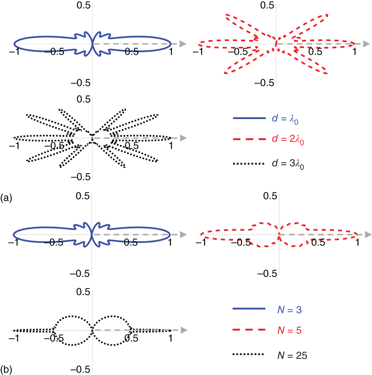
Figure 12.5 Engineering the statistics of the emitted photon by tuning the array geometry. Normalized second‐order angular correlation function  evaluated with
  for a linear vertical array. (a)
  elements with separation distances
  ,
,  and
and  . (b) A separation distance
  and arrays with
  ,
,  , and
, and  emitters. Gray dashed arrow indicates the direction of
  in each subpanel.
12.4.3  ‐Order Correlations
Examining more closely the generalized array factor Eq. (12.40), it is clear that computing the photon statistics becomes a very challenging task as the order increases. Having addressed the first‐ and second‐order correlations, here we address the ![]() ‐order photon correlations for an antenna array in which all emitters are initially excited, i.e. for which
‐order photon correlations for an antenna array in which all emitters are initially excited, i.e. for which
It is the highest‐order nonzero correlation for an array of ![]() single photon sources. Interestingly, a tractable expression can be derived for this extreme case.
single photon sources. Interestingly, a tractable expression can be derived for this extreme case.
The main difficulty in computing the photon statistics stems from evaluating the ![]() ‐order correlator:
‐order correlator:
In order to evaluate the correlator, let ![]() with
with ![]() be a basis for all possible states available to the array of
be a basis for all possible states available to the array of ![]() emitters. This basis can be arbitrary, but for convenience we define the first state of this basis as all emitter's being in the ground state, i.e.
emitters. This basis can be arbitrary, but for convenience we define the first state of this basis as all emitter's being in the ground state, i.e. ![]() . Next, we find the following identity
. Next, we find the following identity

We then make use of the identity operator ![]() to evaluate Eq. (12.52) as follows
to evaluate Eq. (12.52) as follows
where we define ![]() for
for ![]() and
and ![]() in the rest of the cases.
in the rest of the cases.
With this result, the generalized quantum array factor can be written as

Consequently, the definition of ![]() implies that the sum in Eq. (12.53) runs over all possible permutations of the
implies that the sum in Eq. (12.53) runs over all possible permutations of the ![]() position vectors of the following product of exponentials:
position vectors of the following product of exponentials:
For the example of three emitters used in this chapter, the generalized array factor is explicitly:
This result can be understood intuitively in terms of the “which‐path” information that is available in the state of the quantum emitter subsystem. After measuring a ![]() ‐photon coincidence event, the emitter's subsystem must necessarily be in the ground state,
‐photon coincidence event, the emitter's subsystem must necessarily be in the ground state, ![]() . Therefore, the state of the emitters contain no information in terms of what emitter radiated the photon measured at a given detector. In other words, there is no which‐path information and, hence, quantum interference can occur. In this manner, each of the permutations in (12.40) can be understood as a different path that connects the detection in each
. Therefore, the state of the emitters contain no information in terms of what emitter radiated the photon measured at a given detector. In other words, there is no which‐path information and, hence, quantum interference can occur. In this manner, each of the permutations in (12.40) can be understood as a different path that connects the detection in each ![]() direction to the emitter in the
direction to the emitter in the ![]() location. For these reasons, computing the photon statistics become “simpler.” This result also shows that the directivity of the photon statistics is expected to increase along with their order since less and less which‐path information is available as more photons are measured (see Figure 12.3).
location. For these reasons, computing the photon statistics become “simpler.” This result also shows that the directivity of the photon statistics is expected to increase along with their order since less and less which‐path information is available as more photons are measured (see Figure 12.3).
12.5 Isotropic Single‐Photon Sources
We provide in this section yet another example of a quantum antenna device with functionalities that cannot be obtained with a classical antenna system. In particular, we demonstrate that it is possible to have a perfectly isotropic and temporally coherent single‐photon source with full‐polarization coverage [44]. Isotropic antennas are used as a reference in the very definition of directivity. However, it is a well‐known result from classical antenna theory that perfectly isotropic and temporally coherent radiators are not possible [45–48]. This conclusion is best visualized by the hairy ball theorem [49, 50], an algebraic topology result stating that there is no nonvanishing continuous tangent vector field over the entire surface of a sphere. In other words, “you cannot comb a hairy ball flat without creating a cowlick.” Therefore, perfect isotropy with a well‐defined polarization is impossible.
Despite this impossibility, antenna designers continue to seek efficient quasi‐isotropic antennas that approximate the properties of an isotropic radiator [51–54]. The motivation behind quasi‐isotropic antennas is that they provide full‐coverage, an invaluable property for any wireless technology in which transmitting and receiving devices cannot be aligned [55–57]. As a separate note, isotropic sources do exist in the form of thermal radiators [22], and multifrequency systems [58], at the cost of being temporally incoherent. Beyond electromagnetic systems, isotropic sources do exist in other physical systems such as in acoustics [59].
Nevertheless, an isotropic single‐photon source can be designed by using the emitter schematically depicted in Figure 12.6. It consists of a multi‐level system with a single excited state ![]() , and
, and ![]() different ground states
different ground states ![]() . The transition from the excited state to each ground place is characterized by the transition frequency
. The transition from the excited state to each ground place is characterized by the transition frequency ![]() and the dipole moment
and the dipole moment ![]() . The electric field operator takes the same form as that derived for an array of quantum emitters, albeit with all the emitters being located at the same position. Consequently, Eq. (12.38) reduces to
. The electric field operator takes the same form as that derived for an array of quantum emitters, albeit with all the emitters being located at the same position. Consequently, Eq. (12.38) reduces to


Figure 12.6 Isotropic single photon sources. (a) Emitter level structure showing a single excited state connected via radiative transitions to a set of degenerate ground states. (b) Coordinate system and polarization basis. Emission of a photon into the direction  , whose polarization is described by the transverse zenith
  and azimuthal
  vectors, or, equivalently, by an arbitrary polarization basis composed of two orthogonal vectors
  and
and  .
.
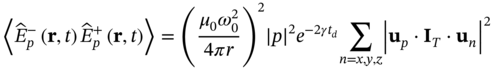
The probability density of measuring a photon with polarization ![]() at the position
at the position ![]() and time
and time ![]() is given by Eq. (12.33). For the multi‐level emitter under consideration it can be explicitly written as
is given by Eq. (12.33). For the multi‐level emitter under consideration it can be explicitly written as

Again, the nonclassical properties of the emission pattern in the proposed configuration arise from the ![]() correlators in Eq. (12.57). In contrast with the classical case, the correlation does not need to be decomposed into the product of two complex numbers, opening up additional degrees of freedom. For a multi‐level emitter with a single excited state and multiple ground states, we have that
correlators in Eq. (12.57). In contrast with the classical case, the correlation does not need to be decomposed into the product of two complex numbers, opening up additional degrees of freedom. For a multi‐level emitter with a single excited state and multiple ground states, we have that ![]() . Interestingly, the result of such a correlator is that there is no interference between the field operators associated with each transition. The absence of interference can be intuitively understood as the result of having distinguishable ground states and thus access to perfect which‐path information. In this sense, the distinguishable ground states play the same role as passive observers similar to popular effects such as two‐slit experiments [60] and quantum erasers [61, 62].
. Interestingly, the result of such a correlator is that there is no interference between the field operators associated with each transition. The absence of interference can be intuitively understood as the result of having distinguishable ground states and thus access to perfect which‐path information. In this sense, the distinguishable ground states play the same role as passive observers similar to popular effects such as two‐slit experiments [60] and quantum erasers [61, 62].
The lack of interference is a nonclassical property arising from the superposition of distinguishable decay paths. It can be harnessed to design an isotropic single‐photon source. To this end, we particularize the multi‐level emitter to the case with three degenerate ground‐states with the same transition frequency (![]() ) and with transition dipole moments of the same magnitude (
) and with transition dipole moments of the same magnitude (![]() ), but oriented along each of the Cartesian axis, i.e.
), but oriented along each of the Cartesian axis, i.e. ![]() ,
, ![]() and
and ![]() . For this configuration, the field correlation reduces to
. For this configuration, the field correlation reduces to
In order to show that the emission will be isotropic for all arbitrary polarizations, we recall that an arbitrary polarization basis ![]() can be obtained from the usual
can be obtained from the usual ![]() basis via rotation by an angle
basis via rotation by an angle ![]() and the introduction a phase shift
and the introduction a phase shift ![]() (see Figure 12.6):
(see Figure 12.6):
By using this decomposition, the probability density of measuring a photon with arbitrary polarization ![]() at time
at time ![]() and location
and location ![]() is found to be:
is found to be:
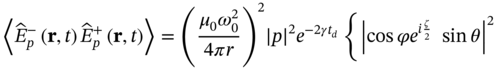

Equation (12.61) reveals that the probability density of detecting a photon is independent of the measurement direction, which is described by the angles ![]() and
and ![]() . Therefore, it can be concluded that the emission is isotropic, i.e. the same probability is obtained for all directions. Moreover, since the probability density is independent of the choice of the polarization vector
. Therefore, it can be concluded that the emission is isotropic, i.e. the same probability is obtained for all directions. Moreover, since the probability density is independent of the choice of the polarization vector ![]() , it can also be concluded that the same result holds for all polarizations. In this manner, it is demonstrated that a perfectly isotropic and with full polarization coverage single‐photon source does exist.
, it can also be concluded that the same result holds for all polarizations. In this manner, it is demonstrated that a perfectly isotropic and with full polarization coverage single‐photon source does exist.
The emission from an isotropic single‐photon source resembles black‐body radiation from a heated object, i.e. the emitted radiation is both isotropic and unpolarized. The main difference is that isotropic single‐photon sources are coherent radiators. Thus, the emitted light corresponds to a single photon with a well‐defined wavepacket. For this reason, it is a coherent source for which interference phenomena can be observed. For example, interference fringes will appear if the emitted photon is sent through a Mach–Zehnder interferometer. In conclusion, isotropic single‐photon sources are a quantum light source with properties that cannot be obtained with classical antennas.
12.6 Quantum Superdirectivity?
It was shown in earlier sections of this chapter that quantum antenna systems provide access to radiation patterns as the average number of photons per direction that cannot be obtained with classical antenna systems. This poses the question of whether or not quantum sources can be used to increase the directivity of antenna systems beyond their classical limits, leading to quantum superdirectivity. A simple proof seems to indicate that this is not possible [63]. However, researchers are known for relentlessly searching for ways to circumvent fundamental limits, and the situation might change in the future. Since the proof provides an additional insight into the mode of operation of quantum antenna arrays, we quickly reproduce it here.
For the sake of simplicity let us consider here an array of all identical emitters, even though the proof can be generalized to more complex scenarios. The starting point is then the first‐order time‐integrated correlation function – the average number of photons measured along the direction ![]() – discussed previously:
– discussed previously:
where ![]() is the first‐order generalized array factor:
is the first‐order generalized array factor:

The classical case is recovered for ![]() . On the other hand,
. On the other hand, ![]() does not need to be factorized as the product of two complex numbers for a quantum antenna array. Again, as a consequence, it provides additional degrees of freedom.
does not need to be factorized as the product of two complex numbers for a quantum antenna array. Again, as a consequence, it provides additional degrees of freedom.
It was shown in Section 12.5 that such freedom can be used to design an isotropic single‐photon source. At the same time, the initial‐time correlation ![]() has some restrictions that limit the achievable radiation patterns. To this end, we define a matrix
has some restrictions that limit the achievable radiation patterns. To this end, we define a matrix ![]() with elements
with elements ![]() and a vector
and a vector ![]() with elements
with elements ![]() . We use them to express
. We use them to express ![]() in matrix form as:
in matrix form as:
In contrast, the radiation pattern of a classical antenna array would be restricted to the more constrained form
Nevertheless, quantum antenna arrays also have some restrictions of their own. First, we note that ![]() and, hence,
and, hence, ![]() is a Hermitian matrix. In addition, since
is a Hermitian matrix. In addition, since ![]() is a positive real number, we then have that
is a positive real number, we then have that ![]() is a positive semidefinite matrix. Importantly, this implies that all its eigenvalues are positive. Next, let
is a positive semidefinite matrix. Importantly, this implies that all its eigenvalues are positive. Next, let ![]() and
and ![]() ,
, ![]() , be the eigenvalues and associated eigenvectors of
, be the eigenvalues and associated eigenvectors of ![]() . Then the spectral decomposition of
. Then the spectral decomposition of ![]() is given by
is given by

Subsequently, ![]() can be rewritten as:
can be rewritten as:
Equation (12.67) reveals that the quantum generalized array factor describing the average number of photons measured as a function of the direction can be written as a linear combination of classical power patterns for the same array, but with different driving coefficients. From this perspective, the power behind quantum antenna arrays is that they enable the superposition of classical power radiation patterns. However, since ![]() is a positive definite matrix, its eigenvalues
is a positive definite matrix, its eigenvalues ![]() must be positive. Therefore, there cannot be destructive interference between the classical radiation patterns. This fact suggests that the directivity cannot be increased by the superposition. In many senses, the situation is very similar to polarization considerations in the maximization of the directivity of classical antennas [64]. The polarization degrees of freedom provide orthogonal channels in which the power can be distributed. However, they cannot be used to increase the directivity.
must be positive. Therefore, there cannot be destructive interference between the classical radiation patterns. This fact suggests that the directivity cannot be increased by the superposition. In many senses, the situation is very similar to polarization considerations in the maximization of the directivity of classical antennas [64]. The polarization degrees of freedom provide orthogonal channels in which the power can be distributed. However, they cannot be used to increase the directivity.
To demonstrate this explicitly, we first define the quantum directivity as follows:
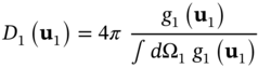

Next, if we optimize the ![]() coefficients, we would obtain the same optimal coefficients for any
coefficients, we would obtain the same optimal coefficients for any ![]() , and therefore the sums in the numerator and denominator would compensate in obtaining the maximal directivity. Consequently, the directivity of a quantum antenna array in terms of the average number of photons cannot exceed the upper limit for a classical antenna array.
, and therefore the sums in the numerator and denominator would compensate in obtaining the maximal directivity. Consequently, the directivity of a quantum antenna array in terms of the average number of photons cannot exceed the upper limit for a classical antenna array.
12.7 Quantum Antenna Array Technologies
Having described the basic theory and its particularly interesting outcomes, we discuss in this section those material platforms that are currently the most promising candidates for implementing quantum antenna arrays. First, the basis of a quantum antenna array is the single‐photon sources that act as their individual elements. The history of single‐photon sources dates back to the 1970s with the first demonstration of a single‐photon source based on a beam of sodium atoms [23]. This effort was followed a decade later by experiments with trapped ions [65]. The first solid‐state single‐photon source was demonstrated in the 1990s using a single molecule dye trapped in a solid [66]. Since then, research on single‐photon sources has exploded, leading to their rapid development. Today, there is a variety of solid‐state single‐photon sources in the form of quantum dots (QDs) [67–70]; color centers in semiconductors, such as diamond, silicon carbide, and silicon [71–76]; and defects in two‐dimensional (2D) materials [77–80]. In general, solid‐state sources suffer from their coupling to a complex environment, e.g. phonons in a crystal lattice, charge accumulations, and interactions with nearby spins. This coupling limits their coherence times. Moreover, it poses difficulties in the fabrication of identical emitters. However, the quality of solid‐state single‐photon sources has been steadily improving and is rapidly approaching the required standards in terms of purity, indistinguishability and on‐demand operation.
Free from a disturbing environment, ultra‐cold atoms [81, 82] and trapped ions [83] are excellent single‐photon sources. Atomic‐based sources provide better single‐photon performance, longer coherence times and a finer control over the photon's wavepacket than their solid‐state counterparts do. Nevertheless, the integration of atomic‐based devices into commercial systems is likely to be restricted to very high‐end applications. Superconducting circuits [84, 85] exhibit the best performance in terms of the coupling strength to the environment and their coherence times. However, the low energy of microwave photons forces these circuits to operate at very low temperatures. The entire system must be contained within a cryogenic setup. Furthermore, nonlinear processes such as spontaneous parametric down conversion were identified early as very high quality nonclassical light sources [86–88], albeit at the cost of being bulky and nondeterministic in nature.
It must be noted that single‐photon sources seldom consist of a quantum emitter alone. The pioneering work of Purcell [89] showed that emission processes are affected by their photonic environments. Subsequently, the use of nanostructures to tailor light‐matter interactions and to enhance the performance of single‐photon sources has been aggressively pursued [69, 90]. Different strategies include the use of resonant cavities [91], a field usually referred to as cavity QED [90]. The resonant interaction with a cavity mode increases the brightness and efficiency of the source, locks the emitted photons into a well‐defined mode, and empowers the observation of reversible decay dynamics in the strong coupling regime. Commonly used resonators include nanopillars [92], nanodisks [93], photonic crystal [94, 95], superconducting [96], and plasmonic [97, 98] cavities. More recently, attention has been partially shifted to the integration of quantum emitters into waveguides [99–101]. Waveguides exhibit advantages similar to cavities in terms of the coupling efficiency to a specific mode and the Purcell enhancement associated with slow light, while at the same time providing intrinsic long‐range interactions that enable the exploration of collective effects [102, 103]. Light emission can not only be enhanced, but also suppressed by the environment. Examples include photonic crystals that exhibit a band gap [104, 105], closed cavities far from resonance [106, 107] and near‐zero‐index (NZI) media [108–111] which lead to the excitation of bound states [112–114] and the associated many‐body physics [115].
Beyond the design of individual emitters, the deterministic fabrication of arrays of quantum emitters with control over their position, orientation, and emission frequency still poses important technological challenges. Again, the most advanced technology is that of atomic‐based emitters. Intensive research on the trapping and cooling of atoms in atomic physics has enabled the deterministic generation of arrays of quantum emitters with hundreds of elements, including one‐dimensional (1D) [116], two‐dimensional (2D) [117], and three‐dimensional (3D) [118, 119] topologies with quite arbitrary geometries. Additional advantages of atomic‐based systems are that all emitters are ensured to be identical, and the initialization and coherent control of the quantum state of the array is much more advanced. We believe that all of the theory presented in earlier sections of this chapter is within the reach of atomic‐based technologies.
Unfortunately, atomic physics setups are not a viable option for most practical applications, and research is needed in the fabrication of quantum antenna arrays in solid‐state platforms. However, the fabrication of arrays of solid‐state emitters is much more challenging. As solid‐state emitters mostly consist of defects in a solid, the interaction with the complex solid‐state environment makes it very difficult to obtain identical emitters with the same orientation, emission wavelength, linewidth, etc. The accurate positioning of the emitters is also a challenging task. Nevertheless, there have been some promising demonstrations of arrays of color centers based on selectively growing on arrays of diamond nanopillars and nanopyramids [120, 121]. Moreover, emitters based on atomically‐thin semiconductors, e.g. tungsten diselenide (![]() ) and hexagonal boron nitride (hBN), are currently showing the most promising advances toward the deterministic fabrication of arrays of solid‐state quantum emitters. In an atomically‐thin semiconductor, an emitter at a specific location can be induced by using nanostructures producing local strains [78, 122, 123], as well as by laser [124] and electron beam [125] irradiation. With these fabrication techniques, we believe that planar quantum antenna arrays based on atomically‐thin semiconductors should be feasible in the short term.
) and hexagonal boron nitride (hBN), are currently showing the most promising advances toward the deterministic fabrication of arrays of solid‐state quantum emitters. In an atomically‐thin semiconductor, an emitter at a specific location can be induced by using nanostructures producing local strains [78, 122, 123], as well as by laser [124] and electron beam [125] irradiation. With these fabrication techniques, we believe that planar quantum antenna arrays based on atomically‐thin semiconductors should be feasible in the short term.
12.8 Forward‐Looking Directions
This chapter has outlined the basic theory of quantum antenna arrays, establishing connections with the antenna theory field whenever possible. While multiple opportunities can be identified at the fundamental and technological levels, quantum antenna arrays are still a nascent field, and it is difficult to predict how it will evolve in the following years. At the fundamental level, it has been demonstrated that quantum antenna arrays enable directional correlations that cannot be achieved with classical systems. However, the complete set of available correlations in the quantum regime is not known, and their impact on physical observables is yet to be discovered. Note that we have used a simple two‐level system model for the emitters. We have not discussed how information would be encoded in the photons emitted by them. Research on more complex emitters, e.g. emitters with a non‐dipolar current distributions and/or multi‐particle transitions, is likely to facilitate even better performance characteristics and other nontrivial phenomena. Information on the emitted photons might be encoded by using polarization and/or temporal control over them. At the same time, the directional correlations induced by the initial state of the systems are a form of embedded information that could be investigated for some practical information exchanges, i.e. communication‐enabled applications. In general, we anticipate that in the next years there will be a large number of theoretical efforts both at the very basic level, as well as in the development of design and synthesis procedures for quantum antenna arrays.
From a practical standpoint, technological applications of quantum antenna arrays are yet to be explored. Classical antenna arrays radiate into free‐space, being the basis of wireless technologies. However, current photonic quantum technologies are mostly based on guided platforms such as optical fibers and photonic integrated circuits. The main reason for the predominant use of guided setups is that these quantum optical systems utilize single or a very reduced number of photons. Therefore, propagation photon losses can be prohibitively high for most applications. Nevertheless, aggressive investments on quantum experiments at the space scale are being funded by state agencies, including the recent demonstrations of satellite QKD distribution, seem to indicate that there will be a future for wireless quantum communications.
We expect that the benefits of wireless connections will also be exploited at small scales and within integrated systems. For example, quantum sensing technologies based on solid‐state spins rely on their optical readout. Currently, optical readout tasks are carried out with bulky far field optics, an approach that is incompatible with a practical implementation outside the laboratory. They need to be addressed in a wireless fashion. Optical antenna arrays might solve this problem by enabling compact and efficient interfaces between solid‐state spins and integrated photonics. Moreover, with the size of solid‐state spins being at the atomic scale, dense arrays of spins cannot be individually resolved with far‐field optics. Having the need to address a sample with many of these emitters, quantum antenna array theory is likely to be needed for the design of advanced optical interfaces, where quantum correlations might be harnessed to improve the performance of their readout.
These are only a few examples of how future directions might look like for quantum antenna arrays. We re‐emphasize that quantum antenna arrays are an emerging field of science and engineering. Many aspects and applications are yet to be explored both from the fundamental and technology perspectives. There are numerous opportunities for electromagnetic researchers with quantum analysis, simulation, and measurement experiences to contribute their skills to this nascent field.
References
- 1 M. F. Riedel, D. Binosi, R. Thew, and T. Calarco, “The European quantum technologies flagship programme,” Quantum Sci. Technol., vol. 2, no. 3, 030501, 2017.
- 2 V. Scarani, H. Bechmann‐Pasquinucci, N. J. Cerf, M. Dušek, N. Lütkenhaus, and M. Peev, “The security of practical quantum key distribution,” Rev. Mod. Phys., vol. 81, no. 3, pp. 1301–1350, 2009.
- 3 Id Quanqique, https://www.idquantique.com.
- 4 Magiq, https://www.magiqtech.com.
- 5 Quintessence labs, https://www.quintessencelabs.com/.
- 6 S.‐K. Liao, W.‐Q. Cai, W.‐Y. Liu, L. Zhang, Y. Li, J.‐G. Ren, J. Yin, Q. Shen, Y. Cao, Z.‐P. Li et al., “Satellite‐to‐ground quantum key distribution,” Nature, vol. 549, no. 7670, pp. 43–47, 2017.
- 7 J. Aasi, J. Abadie, B. P. Abbott, R. Abbott, T. D. Abbott, M. R. A., C. Adams, T. Adams, P. Addesso, R. X. Adhikari et al., “Enhanced sensitivity of the LIGO gravitational wave detector by using squeezed states of light,” Nat. Photonics, vol. 7, no. 8, pp. 613–619, 2013.
- 8 D. A. Simpson, E. Morrisroe, J. M. McCoey, A. H. Lombard, D. C. Mendis, F. Treussart, L. T. Hall, S. Petrou, and L. C. L. Hollenberg, “Non‐neurotoxic nanodiamond probes for intraneuronal temperature mapping,” ACS Nano, vol. 11, no. 12, pp. 12077–12086, 2017.
- 9 D. Le Sage, K. Arai, D. R. Glenn, S. J. DeVience, L. M. Pham, L. Rahn‐Lee, M. D. Lukin, A. Yacoby, A. Komeili, and R. L. Walsworth, “Optical magnetic imaging of living cells,” Nature, vol. 496, no. 7446, pp. 486–489, 2013.
- 10 I. Lovchinsky, A. O. Sushkov, E. Urbach, N. P. de Leon, S. Choi, K. De Greve, R. Evans, R. Gertner, E. Bersin, C. Müller et al., “Nuclear magnetic resonance detection and spectroscopy of single proteins using quantum logic,” Science, vol. 351, no. 6275, pp. 836–841, 2016.
- 11 F. Ziem, M. Garsi, H. Fedder, and J. Wrachtrup, “Quantitative nanoscale MRI with a wide field of view,” Sci. Rep., vol. 9, no. 1, pp. 1–9, 2019.
- 12 J. I. Cirac, “Quantum computing and simulation: Where we stand and what awaits US,” Nanophotonics, vol. 10, no. 1, pp. 453–456, 2020.
- 13 Psiquantum, https://psiquantum.com/.
- 14 Xanadu, https://www.xanadu.ai/.
- 15 H.‐S. Zhong, H. Wang, Y.‐H. Deng, M.‐C. Chen, L.‐C. Peng, Y.‐H. Luo, J. Qin, D. Wu, X. Ding, Y. Hu et al., “Quantum computational advantage using photons,” Science, vol. 370, no. 6523, pp. 1460–1463, 2020.
- 16 W. Vogel and D.‐G. Welsch, Quantum Optics. John Wiley & Sons, 2006.
- 17 T. G. Philbin, “Canonical quantization of macroscopic electromagnetism,” New J. Phys., vol. 12, no. 12, 123008, 2010.
- 18 S. Scheel and S. Y. Buhmann, “Macroscopic QED‐concepts and applications,” arXiv preprint arXiv:0902.3586, 2009.
- 19 S. Y. Buhmann, D. T. Butcher, and S. Scheel, “Macroscopic quantum electrodynamics in nonlocal and nonreciprocal media,” New J. Phys., vol. 14, no. 8, 083034, 2012.
- 20 I. Liberal, I. Ederra, and R. W. Ziolkowski, “Control of a quantum Emitter's bandwidth by managing its reactive power,” Phys. Rev. A, vol. 100, no. 2, 023830, 2019.
- 21 C.‐T. Tai, Dyadic Green Functions in Electromagnetic Theory. IEEE Press, 1994.
- 22 K. Joulain, J.‐P. Mulet, F. Marquier, R. Carminati, and J.‐J. Greffet, “Surface electromagnetic waves thermally excited: Radiative heat transfer, coherence properties and Casimir forces revisited in the near field,” Surf. Sci. Rep., vol. 57, no. 3–4, pp. 59–112, 2005.
- 23 H. J. Kimble, M. Dagenais, and L. Mandel, “Photon antibunching in resonance fluorescence,” Phys. Rev. Lett., vol. 39, no. 11, pp. 691–695, 1977.
- 24 J. F. Clauser, “Experimental distinction between the quantum and classical field‐theoretic predictions for the photoelectric effect,” Phys. Rev. D, vol. 9, no. 4, pp. 853–860, 1974.
- 25 A. Aspect, J. Dalibard, and G. Roger, “Experimental test of Bell's inequalities using time‐varying analyzers,” Phys. Rev. Lett., vol. 49, no. 25, pp. 1804–1807, 1982.
- 26 A. Garg and N. D. Mermin, “Detector inefficiencies in the Einstein‐Podolsky‐Rosen experiment,” Phys. Rev. D, vol. 35, no. 12, pp. 3831–3835, 1987.
- 27 P. H. Eberhard, “Background level and counter efficiencies required for a loophole‐free Einstein‐Podolsky‐Rosen experiment,” Phys. Rev. A, vol. 47, no. 2, pp. R747–R750, 1993.
- 28 J. Barrett, D. Collins, L. Hardy, A. Kent, and S. Popescu, “Quantum nonlocality, bell inequalities, and the memory loophole,” Phys. Rev. A, vol. 66, no. 4, 042111, 2002.
- 29 B. Hensen, H. Bernien, A. E. Dréau, A. Reiserer, N. Kalb, M. S. Blok, J. Ruitenberg, R. F. L. Vermeulen, R. N. Schouten, C. Abellán et al., “Loophole‐free bell inequality violation using electron spins separated by 1.3 kilometres,” Nature, vol. 526, no. 7575, pp. 682–686, 2015.
- 30 L. K. Shalm, E. Meyer‐Scott, B. G. Christensen, P. Bierhorst, M. A. Wayne, M. J. Stevens, T. Gerrits, S. Glancy, D. R. Hamel, M. S. Allman et al., “Strong loophole‐free test of local realism,” Phys. Rev. Lett., vol. 115, no. 25, 250402, 2015.
- 31 M. Giustina, M. A. M. Versteegh, S. Wengerowsky, J. Handsteiner, A. Hochrainer, K. Phelan, F. Steinlechner, J. Kofler, J.‐Å. Larsson, C. Abellán et al., “Significant‐loophole‐free test of Bell's theorem with entangled photons,” Phys. Rev. Lett., vol. 115, no. 25, 250401, 2015.
- 32 R. Loudon, The Quantum Theory of Light. OUP Oxford, 2000.
- 33 R. J. Glauber, “Photon correlations,” Phys. Rev. Lett., vol. 10, no. 3, pp. 84–86, 1963.
- 34 R. J. Glauber, “The quantum theory of optical coherence,” Phys. Rev., vol. 130, no. 6, pp. 2529–2539, 1963.
- 35 P. L. Kelley and W. H. Kleiner, “Theory of electromagnetic field measurement and photoelectron counting,” Phys. Rev., vol. 136, no. 2A, pp. A316–A334, 1964.
- 36 H. J. Carmichael, Statistical Methods in Quantum Optics 2: Non‐Classical Fields. Springer Science & Business Media, 2009.
- 37 C. A. Balanis, Antenna Theory: Analysis and Design. John Wiley & Sons, 2005.
- 38 R. C. Hansen, Phased Array Antennas, vol. 213. John Wiley & Sons, 2009.
- 39 R. J. Mailloux, Phased Array Antenna Handbook, vol. 2. Boston, MA: Artech House, 2005.
- 40 P.‐S. Kildal, Foundations of Antenna Engineering: A Unified Approach for Line‐of‐sight and Multipath. Artech House, 2015.
- 41 A. Predojević and M. W. Mitchell, Engineering the Atom‐Photon Interaction. Springer, 2015.
- 42 M. Saffman, T. G. Walker, and K. Mølmer, “Quantum information with Rydberg atoms,” Rev. Mod. Phys., vol. 82, no. 3, pp. 2313–2363, 2010.
- 43 A. Grankin, D. V. Vasilyev, P. O. Guimond, B. Vermersch, and P. Zoller, A ‘few‐atom’ quantum optical antenna. arXiv preprint arXiv:1802.05592, 2018.
- 44 I. Liberal, I. Ederra, and Y. Li, “Isotropic single‐photon sources,” Opt. Lett., vol. 43, no. 12, pp. 2736–2739, 2018.
- 45 H. F. Mathis, “A short proof that an isotropic antenna is impossible,” Proc. IRE, vol. 39, p. 970, 1951.
- 46 W. K. Saunders, “On the Unity Gain Antenna,” in Electromagnetic Theory and Antennas, vol. 2, E. C. Jordan, Ed. Pergamon Press, 1963.
- 47 W. Scott and K. Soo Hoo, “A theorem on the polarization of null‐free antennas,” IEEE Trans. Antennas Propag., vol. 14, no. 5, pp. 587–590, 1966.
- 48 H. Matzner and K. T. McDonald, “Isotropic radiators,”. arXiv preprint physics/0312023, 2003.
- 49 P. Renteln, Manifolds, Tensors, and Forms: An Introduction for Mathematicians and Physicists. Cambridge University Press, 2013.
- 50 R. E. Schwartz, Mostly Surfaces, vol. 60. American Mathematical Society, 2011.
- 51 Y. Pan and S. Zheng, “A compact quasi‐isotropic shorted patch antenna,” IEEE Access, vol. 5, pp. 2771–2778, 2017.
- 52 P. Liu, Y. Li, Z. Zhang, and Z. Feng, “Omnidirectional dual‐polarized antenna with sabre‐like structure,” IEEE Trans. Antennas Propag., vol. 65, no. 6, pp. 3221–3225, 2017.
- 53 Q. Li, W.‐J. Lu, S.‐G. Wang, and L. Zhu, “Planar quasi‐isotropic magnetic dipole antenna using fractional‐order circular sector cavity resonant mode,” IEEE Access, vol. 5, pp. 8515–8525, 2017.
- 54 J.‐H. Kim and S. Nam, “A compact quasi‐isotropic antenna based on folded split‐ring resonators,” IEEE Antennas Wireless Propag. Lett., vol. 16, pp. 294–297, 2017.
- 55 Z. N. Chen, X. Qing, T. S. P. See, and W. K. Toh, “Antennas for WiFi connectivity,” Proc. IEEE, vol. 100, no. 7, pp. 2322–2329, 2012.
- 56 S. X. Ta, I. Park, and R. W. Ziolkowski, “Crossed dipole antennas: A review,” IEEE Antennas Propag. Mag., vol. 57, no. 5, pp. 107–122, 2015.
- 57 M. Arrawatia, M. S. Baghini, and G. Kumar, “Broadband bent triangular omnidirectional antenna for RF energy harvesting,” IEEE Antennas Wireless Propag. Lett., vol. 15, pp. 36–39, 2016.
- 58 F. Fulton, “The combined radiation pattern of three orthogonal dipoles,” IEEE Trans. Antennas Propag., vol. 13, no. 2, pp. 323–324, 1965.
- 59 A. D. Yaghjian, “Scattering‐matrix analysis of linear periodic arrays,” IEEE Trans. Antennas Propag., vol. 50, no. 8, pp. 1050–1064, Aug 2002.
- 60 M. O. Scully and M. S. Zubairy, Quantum Optics. Cambridge University Press, 1997.
- 61 M. O. Scully and K. Drühl, “Quantum eraser: A proposed photon correlation experiment concerning observation and “delayed choice” in quantum mechanics,” Phys. Rev. A, vol. 25, no. 4, pp. 2208–2213, 1982.
- 62 Y. Aharonov and M. S. Zubairy, “Time and the quantum: Erasing the past and impacting the future,” Science, vol. 307, no. 5711, pp. 875–879, 2005.
- 63 I. Liberal, I. Ederra, and R. W. Ziolkowski, “Quantum antenna arrays: The role of quantum interference on direction‐dependent photon statistics,” Phys. Rev. A, vol. 97, no. 5, 053847, 2018.
- 64 R. Harrington, “On the gain and beamwidth of directional antennas,” IRE Trans. Antennas Propag., vol. 6, no. 3, pp. 219–225, 1958.
- 65 F. Diedrich and H. Walther, “Nonclassical radiation of a single stored ion,” Phys. Rev. Lett., vol. 58, no. 3, pp. 203–206, 1987.
- 66 Th. Basché, W. E. Moerner, M. Orrit, and H. Talon, “Photon antibunching in the fluorescence of a single dye molecule trapped in a solid,” Phys. Rev. Lett., vol. 69, no. 10, pp. 1516–1519, 1992.
- 67 N. Tomm, A. Javadi, N. O. Antoniadis, D. Najer, M. C. Löbl, A. R. Korsch, R. Schott, S. R. Valentin, A. D. Wieck, A. Ludwig et al., “A bright and fast source of coherent single photons,” Nat. Nanotechnol., vol. 16, no. 4, pp. 399–403, 2021.
- 68 P. Senellart, G. Solomon, and A. White, “High‐performance semiconductor quantum‐dot single‐photon sources,” Nat. Nanotechnol., vol. 12, no. 11, pp. 1026–1039, 2017.
- 69 P. Lodahl, S. Mahmoodian, and S. Stobbe, “Interfacing single photons and single quantum dots with photonic nanostructures,” Rev. Mod. Phys., vol. 87, no. 2, pp. 347–400, 2015.
- 70 S. Buckley, K. Rivoire, and J. Vučković, “Engineered quantum dot single‐photon sources,” Rep. Prog. Phys., vol. 75, no. 12, 126503, 2012.
- 71 M. Atatüre, D. Englund, N. Vamivakas, S.‐Y. Lee, and J. Wrachtrup, “Material platforms for spin‐based photonic quantum technologies,” Nat. Rev. Mater., vol. 3, no. 5, pp. 38–51, 2018.
- 72 D. D. Awschalom, R. Hanson, J. Wrachtrup, and B. B. Zhou, “Quantum technologies with optically interfaced solid‐state spins,” Nat. Photonics, vol. 12, no. 9, pp. 516–527, 2018.
- 73 I. Aharonovich, D. Englund, and M. Toth, “Solid‐state single‐photon emitters,” Nat. Photonics, vol. 10, no. 10, pp. 631–641, 2016.
- 74 S. Castelletto, B. C. Johnson, V. Ivády, N. Stavrias, T. Umeda, A. Gali, and T. Ohshima, “A silicon carbide room‐temperature single‐photon source,” Nat. Mater., vol. 13, no. 2, pp. 151–156, 2014.
- 75 A. Sipahigil, R. E. Evans, D. D. Sukachev, M. J. Burek, J. Borregaard, M. K. Bhaskar, C. T. Nguyen, J. L. Pacheco, H. A. Atikian, C. Meuwly et al., “An integrated diamond nanophotonics platform for quantum‐optical networks,” Science, vol. 354, no. 6314, pp. 847–850, 2016.
- 76 I. Aharonovich and E. Neu, “Diamond nanophotonics,” Adv. Opt. Mater., vol. 2, no. 10, pp. 911–928, 2014.
- 77 M. Toth and I. Aharonovich, “Single photon sources in atomically thin materials,” Annu. Rev. Phys. Chem., vol. 70, pp. 123–142, 2019.
- 78 T. T. Tran, K. Bray, M. J. Ford, M. Toth, and I. Aharonovich, “Quantum emission from hexagonal boron nitride monolayers,” Nat. Nanotechnol., vol. 11, no. 1, pp. 37–41, 2016.
- 79 Y.‐M. He, G. Clark, J. R. Schaibley, Y. He, M.‐C. Chen, Y.‐J. Wei, X. Ding, Q. Zhang, W. Yao, X. Xu et al., “Single quantum emitters in monolayer semiconductors,” Nat. Nanotechnol., vol. 10, no. 6, pp. 497–502, 2015.
- 80 A. Srivastava, M. Sidler, A. V. Allain, D. S. Lembke, A. Kis, and A. Imamoğlu, “Optically active quantum dots in monolayer WSE 2,” Nat. Nanotechnol., vol. 10, no. 6, pp. 491–496, 2015.
- 81 A. Kuhn, M. Hennrich, and G. Rempe, “Deterministic single‐photon source for distributed quantum networking,” Phys. Rev. Lett., vol. 89, no. 6, 067901, 2002.
- 82 J. McKeever, A. Boca, A. D. Boozer, R. Miller, J. R. Buck, A. Kuzmich, and H. J. Kimble, “Deterministic generation of single photons from one atom trapped in a cavity,” Science, vol. 303, no. 5666, pp. 1992–1994, 2004.
- 83 M. Keller, B. Lange, K. Hayasaka, W. Lange, and H. Walther, “Continuous generation of single photons with controlled waveform in an ion‐trap cavity system,” Nature, vol. 431, no. 7012, pp. 1075–1078, 2004.
- 84 A. Wallraff, D. I. Schuster, A. Blais, L. Frunzio, R.‐S. Huang, J. Majer, S. Kumar, S. M. Girvin, and R. J. Schoelkopf, “Strong coupling of a single photon to a superconducting qubit using circuit quantum electrodynamics,” Nature, vol. 431, no. 7005, pp. 162–167, 2004.
- 85 A. A. Houck, D. I. Schuster, J. M. Gambetta, J. A. Schreier, B. R. Johnson, J. M. Chow, L. Frunzio, J. Majer, M. H. Devoret, S. M. Girvin et al., “Generating single microwave photons in a circuit,” Nature, vol. 449, no. 7160, pp. 328–331, 2007.
- 86 F. Kaneda and P. G. Kwiat, “High‐efficiency single‐photon generation via large‐scale active time multiplexing,” Sci. Adv., vol. 5, no. 10, eaaw8586, 2019.
- 87 P. G. Kwiat, K. Mattle, H. Weinfurter, A. Zeilinger, A. V. Sergienko, and Y. Shih, “New high‐intensity source of polarization‐entangled photon pairs,” Phys. Rev. Lett., vol. 75, no. 24, pp. 4337–4341, 1995.
- 88 C. K. Hong and L. Mandel, “Experimental realization of a localized one‐photon state,” Phys. Rev. Lett., vol. 56, no. 1, pp. 58–60, 1986.
- 89 E. M. Purcell, “ Spontaneous emission probabilities at radio frequencies,” in Confined Electrons and Photons. Springer, 1995, p. 839.
- 90 S. Haroche and J.‐M. Raimond, Exploring the Quantum: Atoms, Cavities, and Photons. Oxford University Press, 2006.
- 91 K. J. Vahala, “Optical microcavities,” Nature, vol. 424, no. 6950, pp. 839–846, 2003.
- 92 J. P. Reithmaier, G. Sek, A. Löffler, C. Hofmann, S. Kuhn, S. Reitzenstein, L. V. Keldysh, V. D. Kulakovskii, T. L. Reinecke, and A. Forchel, “Strong coupling in a single quantum dot–semiconductor microcavity system,” Nature, vol. 432, no. 7014, pp. 197–200, 2004.
- 93 K. Srinivasan and O. Painter, “Linear and nonlinear optical spectroscopy of a strongly coupled microdisk–quantum dot system,” Nature, vol. 450, no. 7171, pp. 862–865, 2007.
- 94 T. Yoshie, A. Scherer, J. Hendrickson, G. Khitrova, H. M. Gibbs, G. Rupper, C. Ell, O. B. Shchekin, and D. G. Deppe, “Vacuum Rabi splitting with a single quantum dot in a photonic crystal nanocavity,” Nature, vol. 432, no. 7014, pp. 200–203, 2004.
- 95 K. Hennessy, A. Badolato, M. Winger, D. Gerace, M. Atatüre, S. Gulde, S. Fält, E. L. Hu, and A. Imamoğlu, “Quantum nature of a strongly coupled single quantum dot–cavity system,” Nature, vol. 445, no. 7130, pp. 896–899, 2007.
- 96 S. Kuhr, S. Gleyzes, C. Guerlin, J. Bernu, U. B. Hoff, S. Deléglise, S. Osnaghi, M. Brune, J.‐M. Raimond, S. Haroche et al., “Ultrahigh finesse Fabry‐Pérot superconducting resonator,” Appl. Phys. Lett., vol. 90, no. 16, 164101, 2007.
- 97 G. M. Akselrod, C. Argyropoulos, T. B. Hoang, C. Ciracì, C. Fang, J. Huang, D. R. Smith, and M. H. Mikkelsen, “Probing the mechanisms of large Purcell enhancement in plasmonic nanoantennas,” Nat. Photonics, vol. 8, no. 11, pp. 835–840, 2014.
- 98 R. Chikkaraddy, B. D. Nijs, F. Benz, S. J. Barrow, O. A. Scherman, E. Rosta, A. Demetriadou, P. Fox, O. Hess, and J. J. Baumberg, “Single‐molecule strong coupling at room temperature in plasmonic nanocavities,” Nature, vol. 535, no. 7610, pp. 127–130, 2016.
- 99 M. Arcari, I. Söllner, A. Javadi, S. L. Hansen, S. Mahmoodian, J. Liu, H. Thyrrestrup, E. H. Lee, J. D. Song, S. Stobbe et al., “Near‐unity coupling efficiency of a quantum emitter to a photonic crystal waveguide,” Phys. Rev. Lett., vol. 113, no. 9, 093603, 2014.
- 100 A. V. Akimov, A. Mukherjee, C. L. Yu, D. E. Chang, A. S. Zibrov, P. R. Hemmer, H. Park, and M. D. Lukin, “Generation of single optical plasmons in metallic nanowires coupled to quantum dots,” Nature, vol. 450, no. 7168, pp. 402–406, 2007.
- 101 A. F. Van Loo, A. Fedorov, K. Lalumiere, B. C. Sanders, A. Blais, and A. Wallraff, “Photon‐mediated interactions between distant artificial atoms,” Science, vol. 342, no. 6165, pp. 1494–1496, 2013.
- 102 A. Goban, C.‐L. Hung, J. D. Hood, S.‐P. Yu, J. A. Muniz, O. Painter, and H. J. Kimble, “Superradiance for atoms trapped along a photonic crystal waveguide,” Phys. Rev. Lett., vol. 115, no. 6, 063601, 2015.
- 103 A. Goban, C.‐L. Hung, S.‐P. Yu, J. D. Hood, J. A. Muniz, J. H. Lee, M. J. Martin, A. C. McClung, K. S. Choi, D. E. Chang et al., “Atom–light interactions in photonic crystals,” Nat. Commun., vol. 5, no. 1, pp. 1–9, 2014.
- 104 V. P. Bykov, “Spontaneous emission from a medium with a band spectrum,” Sov. J. Quantum Electron., vol. 4, no. 7, pp. 861–871, 1975.
- 105 E. Yablonovitch, “Inhibited spontaneous emission in solid‐state physics and electronics,” Phys. Rev. Lett., vol. 58, no. 20, pp. 2059–2062, 1987.
- 106 D. Kleppner, “Inhibited spontaneous emission,” Phys. Rev. Lett., vol. 47, no. 4, pp. 233–236, 1981.
- 107 R. G. Hulet, E. S. Hilfer, and D. Kleppner, “Inhibited spontaneous emission by a Rydberg atom,” Phys. Rev. Lett., vol. 55, no. 20, pp. 2137–2140, 1985.
- 108 M. Lobet, I. Liberal, E. N. Knall, M. Z. Alam, O. Reshef, R. W. Boyd, N. Engheta, and E. Mazur, “Fundamental radiative processes in near‐zero‐index media of various dimensionalities,” ACS Photonics, vol. 7, no. 8, pp. 1965–1970, 2020.
- 109 I. Liberal and N. Engheta, “Zero‐index structures as an alternative platform for quantum optics,” Proc. Natl. Acad. Sci. U.S.A., vol. 114, no. 5, pp. 822–827, 2017.
- 110 I. Liberal and N. Engheta, “Nonradiating and radiating modes excited by quantum emitters in open epsilon‐near‐zero cavities,” Sci. Adv., vol. 2, no. 10, e1600987, 2016.
- 111 A. Erentok and R. W. Ziolkowski, “A hybrid optimization method to analyze metamaterial‐based electrically small antennas,” IEEE Trans. Antennas Propag., vol. 55, no. 3, pp. 731–741, 2007.
- 112 S. John and J. Wang, “Quantum electrodynamics near a photonic band gap: Photon bound states and dressed atoms,” Phys. Rev. Lett., vol. 64, no. 20, pp. 2418–2421, 1990.
- 113 S. John and T. Quang, “Spontaneous emission near the edge of a photonic band gap,” Phys. Rev. A, vol. 50, no. 2, pp. 1764–1769, 1994.
- 114 T. Shi, Y.‐H. Wu, A. González‐Tudela, and J. I. Cirac, “Bound states in boson impurity models,” Phys. Rev. X, vol. 6, no. 2, 021027, 2016.
- 115 D. E. Chang, J. S. Douglas, A. González‐Tudela, C.‐L. Hung, and H. J. Kimble, “Colloquium: Quantum matter built from nanoscopic lattices of atoms and photons,” Rev. Mod. Phys., vol. 90, no. 3, 031002, 2018.
- 116 M. Endres, H. Bernien, A. Keesling, H. Levine, E. R. Anschuetz, A. Krajenbrink, C. Senko, V. Vuletic, M. Greiner, and M. D. Lukin, “Atom‐by‐atom assembly of defect‐free one‐dimensional cold atom arrays,” Science, vol. 354, no. 6315, pp. 1024–1027, 2016.
- 117 H. Labuhn, D. Barredo, S. Ravets, S. De Léséleuc, T. Macrì, T. Lahaye, and A. Browaeys, “Tunable two‐dimensional arrays of single Rydberg atoms for realizing quantum Ising models,” Nature, vol. 534, no. 7609, pp. 667–670, 2016.
- 118 D. Barredo, V. Lienhard, S. De Leseleuc, T. Lahaye, and A. Browaeys, “Synthetic three‐dimensional atomic structures assembled atom by atom,” Nature, vol. 561, no. 7721, pp. 79–82, 2018.
- 119 A. Kumar, T.‐Y. Wu, F. Giraldo, and D. S. Weiss, “Sorting ultracold atoms in a three‐dimensional optical lattice in a realization of Maxwell's demon,” Nature, vol. 561, no. 7721, pp. 83–87, 2018.
- 120 T. Jaffe, N. Felgen, L. Gal, L. Kornblum, J. P. Reithmaier, C. Popov, and M. Orenstein, “Deterministic arrays of epitaxially grown diamond nanopyramids with embedded silicon‐vacancy centers,” Adv. Opt. Mater., vol. 7, no. 2, 1800715, 2019.
- 121 J. L. Zhang, K. G. Lagoudakis, Y.‐K. Tzeng, C. Dory, M. Radulaski, Y. Kelaita, K. A. Fischer, S. Sun, Z.‐X. Shen, N. A. Melosh, S. Chu, and J. Vučković, “Complete coherent control of silicon vacancies in diamond nanopillars containing single defect centers,” Optica, vol. 4, no. 11, pp. 1317–1321, Nov 2017.
- 122 C. Palacios‐Berraquero, D. M. Kara, A. R.‐P. Montblanch, M. Barbone, P. Latawiec, D. Yoon, A. K. Ott, M. Loncar, A. C. Ferrari, and A. Mete, “Large‐scale quantum‐emitter arrays in atomically thin semiconductors,” Nat. Commun., vol. 8, 15093, 2017.
- 123 C. Li, N. Mendelson, R. Ritika, Y. L. Chen, Z.‐Q. Xu, M. Toth, and I. Aharonovich, “Scalable and deterministic fabrication of quantum emitter arrays from hexagonal boron nitride,” Nano Lett., vol. 21, no. 8, pp. 3626–3632, 2021.
- 124 S. Hou, M. D. Birowosuto, S. Umar, M. A. Anicet, R. Y. Tay, P. Coquet, B. K. Tay, H. Wang, and E. H. T. Teo, “Localized emission from laser‐irradiated defects in two‐dimensional hexagonal boron nitride,” 2D Materials, vol. 5, pp. 2053–1583, 2017.
- 125 C. Fournier, A. Plaud, S. Roux, A. Pierret, M. Rosticher, K. Watanabe, T. Taniguchi, S. Buil, X. Quélin, J. Barjon et al., “Position‐controlled quantum emitters with reproducible emission wavelength in hexagonal boron nitride,” Nat. Commun., vol. 12, 3779, 2021.