The cost function or loss function is a very important function in machine learning algorithms. Most algorithms have some form of cost function, and the goal is to minimize this. Parameters, which affect cost functions, such as stepSize, are called hyperparameters; they need to be set by hand. Therefore, understanding the whole concept of the cost function is very important.

In this recipe, we are going to analyze the cost function in linear regression. Linear regression is a simple algorithm to understand, and it will help you understand the role of cost functions for even complex algorithms.

Let's go back to linear regression. The goal is to find the best-fitting line so that the mean square of the error would be minimum. Here, we are referring to an error as the difference between the value as per the best-fitting line and the actual value of the response variable of the training dataset.

For a simple case of a single predicate variable, the best-fitting line can be written as:

This function is also called the hypothesis function and can be written as:

The goal of linear regression is to find the best-fitting line. On this line, θ₀ represents the intercept on the y axis, and θ₁ represents the slope of the line, as is obvious from the following equation:

We have to choose θ₀ and θ₁ in a way that h(x) would be closest to y in the case of the training dataset. So, for the i^th data point, the square of the distance between the line and the data point is:

To put it in words, this is the square of the difference between the predicted house price and the actual price the house got sold for. Now, let's take the average of this value across the training dataset:

The preceding equation is called the cost function J for linear regression. The goal is to minimize this cost function:

This cost function is also called the squared error function. Both θ₀ and θ₁ follow a convex curve independently if they are plotted against J.

Let's take a very simple example of a dataset with three values—(1,1), (2,2), and (3,3)—to make the calculation easy:

Let's assume θ₁ is 0, that is, the best-fitting line parallel to the x axis. In the first case, assume that the best-fitting line is the x axis, that is, y=0. In that case, the following will be the value of the cost function:

Move this line up to y=1. The following will be the value of the cost function now:

Now let's move this line further up to y=2. Then, the following will be the value of the cost function:

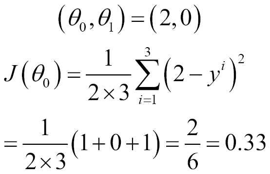
When we move this line further up to y=3, the following will be the value of the cost function:

When we move this line further up to y=4, the following will be the value of the cost function:

So, you saw that the value of the cost function first decreased and then increased again like this:

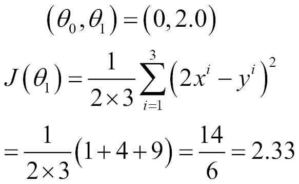
Now let's repeat the exercise by making θ₀ as 0 and using different values of θ₁.

In the first case, assume the best-fitting line is the x axis, that is, y=0. The following will be the value of the cost function in this scenario:

Use a slope of 0.5. The following will be the value of the cost function now:

Now use a slope of 1. The following will be the value of the cost function:

When you use a slope of 1.5, the following will be the value of the cost function:

When you use a slope of 2.0, the following will be the value of the cost function:

As you can see, in both the graphs, the minimum value of J is when the slope or gradient of the curve is 0:

When both θ₀ and θ₁ are mapped to a 3D space, it becomes like the shape of a bowl with the minimum value of the cost function at the bottom of it.

This approach to arrive at the minimum value is called gradient descent. In Spark, the implementation is referred to as this: stochastic gradient descent.