
Lesson Files | Lessons > Lesson_15 > 15_Team_Roster.numbers Lessons > Lesson_15 > 15_Time_Log.numbers Lessons > Lesson_15 > 15_College_Savings.numbers |
Time | This lesson takes approximately 60 minutes to complete. |
Goals | Freeze a header row Organize a table using categories and subcategories Format a table with styles Filter table data Change the formatting of cells for special data types Locate functions with the Function Browser Replace placeholder arguments in a function |
In the two previous lessons, we used tables to organize data and analyze and sort information. In this lesson, we’ll take data analysis a step further, and dive into the finer points of filtering, categorizing, summarizing, and calculating with Numbers spreadsheets. In particular, we’ll use:
Intelligent tables that make it easy to create categories based on your data and summarize the results.
Data filtering, which can help you reorganize data to display specific information.
Powerful formulas, which allow you to calculate a wide range of solutions. With the Function Browser, you can access over 250 functions, including special functions for engineering, statistical, and financial tasks.
Numbers can create useful categories based upon selected columns. In this exercise, we’ll use a roster for a youth baseball league to organize a table into several categories.
We’ll assume the coaches in the league want to know how many players are available for each position as they’re forming teams for the coming season. They also want to sort by the age of the players, so they can start recruiting now for positions where they’ll be short of players in future seasons.
Let’s start by opening the league roster and making it easier to read.
Your league roster has a header row across the top of the table, which of course will appear at the top of each page automatically when you print. But it’s also something you refer to constantly when organizing your information.
So we’ll begin with a handy organizational tool: freezing the header row and header column so that they remain visible while you scroll through the rest of the spreadsheet. By freezing the header row and column, you can always view and refer to those labels, no matter how deep you navigate into your spreadsheet.
Open Numbers if it is not already open.
Choose File > Open and navigate to the Lesson_15 folder.
Select 15_Team_Roster.numbers and click Open.
Numbers opens a spreadsheet that includes two sheets.
Select the first sheet Table Categories, and then click on the table, League Roster.

Scroll down the list to browse the table contents.
As you scroll down, notice that the header row scrolls off the top of the page. It would be more useful if this row were always visible to you as you work.

Choose Table > Freeze Header Rows.

Scroll down the table and notice that the header row remains visible at the top of the table at all times.
You can organize a spreadsheet into categories based upon the values in a single column. For example, in the case of our league roster, you can categorize players by position. This will allow the coaches to organize new teams by viewing how many players they have for each position.
Click column D (Position) to select it.
Click the cell reference pop-up menu and choose Categorize by This Column.

Numbers organizes the data in column D into categories and creates a spreadsheet category for each unique value in the column. The column you used to create categories is the category value column.
Note
Be sure to remove any empty cells in column D, or they will be organized into a (blank) category.

You can take categorizing further by using subcategories. For this table, let’s categorize using player age as a subcategory. This will help the coaches distribute players to new teams based upon both position and age, and maintain a fair balance of players on each team.
Click column B (Age) to select it.
Click the cell reference pop-up menu and choose Sort Ascending to sort the players by age.
Click the cell reference pop-up menu and choose Categorize by This Column.
Numbers creates subcategories for the players’ ages.

The catchers who are 12 years of age are no longer eligible to play in this league, so you have no need to display their names in this roster. You can use categories to address this.
Click the disclosure triangle in the 12 Catcher category subheader.
Numbers hides the catchers who are 12 years old, as they will be too old to play next season.
While this kind of filtering is useful, it can also be applied globally to the table, as you’ll discover in the next exercise.
If your table contains information that you’d like to temporarily hide, you can filter it. This hides the data from view but does not remove it from the table.
In the toolbar, click Reorganize.

The Reorganize window opens. Notice that the sort controls and the categorizing controls are in use. The middle area of the window is used for filtering.
If the filtering controls are not visible in the Reorganize window, click the Filter disclosure triangle to display them.
From the “Choose a column” pop-up menu, choose Age.

Tip
You can create new filter criteria by clicking the Add (+) button and defining each column you want to insert.
You can now choose specific data values to display in your spreadsheet.
Change the pop-up menu labeled is to is not; then type 12 in the value field and press Return.

Numbers filters all results to show information for only those rows that do not contain an age value of 12.
Close the Reorganize window.
Let’s count how many players you have available for each position.
Click cell D3 to select the position subcategory.
Click the disclosure triangle for D3, and choose Count.

Numbers calculates how many players of each age are available for each position.
Choose File > Close and save your work.
You have formatted a table to show only that information you require. Additionally, when you use categories, the information in your table becomes easier to sort and view.
As you’ve seen, table categories make it easier to organize and review information. In the next exercises, we’ll use categories and other advanced functions to create a time log. This report is useful for those who bill their time hourly or track time usage.
While Numbers makes your information easy to read, it can also format a table so that it is print ready. By applying table styles and formatting, you can turn a raw spreadsheet into a report that is ready to give to a client.
Let’s get started by opening the original time log.
Choose File > Open and navigate to the Lesson_15 folder.
Select 15_Time_Log.numbers and click Open.
Numbers opens a spreadsheet with two sheets attached.
Select the first sheet, Time Log Start.

This table contains an employee-tracking sheet. Maintaining this sheet is an easy way to track the time spent on specific tasks. Let’s clean up the table by removing empty space.
Click a cell in the table to select it. Then drag the Column and Row handle up to remove empty rows. You should end up with 30 rows and 4 columns.

Click column C (Task); then click the cell reference pop-up menu and choose Categorize by This Column.

Numbers categorizes the data according to tasks performed. Let’s further improve the appearance of the table.
In the Styles list, click Beige to reformat the table’s appearance.

Great—the table looks very professional and easy to read. Let’s now use a variable, “billable,” to total the number of hours the employee can bill his client.
In the current project, not every hour worked is billable. Some of the employee’s time was “internal,” which does not produce income but is worth tracking for future planning and analysis. Let’s calculate only the number of billable hours.
Examine column A.

You’ll notice that it contains checkboxes for each task. This is a useful way to format a cell so that its value indicates one of two states.
Click column D to select it.
This column contains the actual time spent. The employee typed the letter m after the number data to indicate that the value represents minutes.
w—weeks
d—days
h—hours
m—minutes
s—seconds
ms—milliseconds
Click the cell reference pop-up menu and choose Add Column After.
Enter Billable Time in the header row for column E.

You now can calculate the number of billable hours by creating a simple formula.
Click cell E3 to add a formula because this is the first row with actual data in both the Time and Billable columns.
Press the = (equal sign) key to open the Formula Editor.
Click cell A3, press the * (asterisk) key, and then click cell D3.
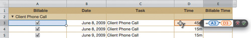
The formula should read =A3*D3.
Press Return to apply the formula.
Because the checkbox is selected, it is treated as a value of 1. If the Billable checkbox is deselected, it is treated as a value of 0.
Click cell E3 to select it, and then drag the blue Fill handle in the lower right corner through cell E36. Numbers now shows the number of billable hours in column E.

Now that all of the billable hours are displayed, you can use that information in another table. Let’s add a second, reporting table to this sheet so that you can compare the total hours worked with the billable hours.
In the toolbar, click the Tables button and choose Sums.

A new table is added to the sheet.
In the Sheets pane, double-click the table name to select it and rename the table Report.
Let’s style this table to match the first table.
Click the Beige button to apply the identical table style. Drag the table so that it is aligned with the first table.
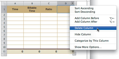
Label the first three header row cells as follows: Time, Billable Time, and Ratio.
Let’s remove the unused column.
Select column D; then click the cell reference pop-up menu and choose Delete Column.
In the Report table, click cell A2. This is where the billable time will be added.
Press the = (equal sign) key to open the Formula Editor.
In the Billable Hours table, drag to select cells D3 through D36.

The formula should read =SUM(Billable Hours :: D3:D36). SUM is a basic function that adds the range of selected cells. You’ll explore functions in depth later in this lesson.
Press Return. The cell should display a value of 2550 minutes.
Let’s perform a similar calculation for the next column.
In the Report table, click cell B2, and then press the = (equal sign) key to open the Formula Editor.
In the Billable Hours table, select cells E3 through E36.
The formula should read =SUM(Billable Hours :: E3:E36).
Press Return. The cell should display a value of 2100 minutes.

Let’s remove the unused cells. Drag up the Column and Row handle for the table so that it is three rows by three columns.

In the Report table, click cell C3 and press the = (equal sign) key.
Enter the following formula: =B3/A3. Press Return.

You have successfully created a new table. By formatting the Report table, you can make displayed values easier to understand.
As you create formulas, you’ll often want to format the way results are displayed to make the information more clear to the reader. In the current table, it would be useful to see the total time spent displayed as hours and the ratio displayed as a percentage.
In the Report table, click cell A3.
Cell A3 is in a footer row and shows the total from the cells in this column. Let’s change the calculated totals from minutes to hours and minutes.
Open the Cells inspector.
From the Cell Format pop-up menu, choose Duration.
You can use the Units control to select the units you want to display for a duration value.
Drag the left end of the slider until it’s over the Hr unit.

The time total is now displayed in hours and minutes, which is more useful to the manager and the accounting department. Let’s reuse this formula in the next column.
Drag the blue Fill handle to the right so that the data in column B is displayed with the same formatting.

All that is left is to improve the percentage display in column C.
Select cell C3.
In the format bar, click the Percentage button to change how the cell displays its contents.
The number is now displayed as 82.35%.

Choose File > Close and save your work.
You have utilized several advanced features, including formatting irregular units like time, in a table.
As you continue to work with formulas, you’ll use functions to perform specific tasks. (For example, you used the SUM and COUNT functions earlier in this lesson.) A function is a predefined, named operation (such as AVERAGE) that can perform a calculation. When writing a formula, you can use multiple functions or just one, depending on the task at hand.
More Info
With more than 250 functions to choose from in Numbers, you might overlook a few useful ones; not everyone who uses Numbers has formal training in accounting or statistics. To help you make the most of functions, Numbers includes a dedicated Help module. To use it, choose Help > iWork Formulas and Functions Help. It contains several example formulas and a detailed reference guide.
Let’s use a function to determine a financial goal for college savings.
Choose File > Open and navigate to the Lesson_15 folder.
Select 15_College_Savings.numbers and click Open.
Numbers opens a spreadsheet with two sheets attached.
Select the College Planning sheet.
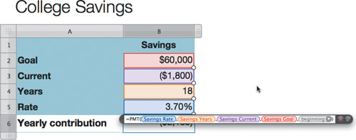
The table on the sheet outlines a target for savings. A family has determined that it wants to set aside $60,000 toward the cost of a daughter’s tuition. Let’s break down the contents of the table.

The family’s savings goal is $60,000, and it currently has $1,800 in the bank. (According to accounting practice, investments are shown in parentheses to represent negative numbers.) The family has 18 years toward its goal because the savings started as soon as a child was on the way. It is expected that an interest rate of 3.7% can be realized by investing the savings.
What the family wants to determine is how much money it has to save each year to realize the college savings goal. Let’s find a function to calculate the annual investment.
Click on table and select cell B6, and in the toolbar, click the Function button. Choose Show Function Browser.
The Function Browser is a convenient way to add a function to a formula.

The browser is organized as follows:
The left pane lists categories of functions so that you can browse by the type of function.
The right pane lists individual functions. Click a function to select it and view information about how to use it.
The lower pane contains detailed information about the selected function.
In the left pane, click Financial; then scroll to examine your choices in the right pane.
The appropriate function choice is PMT, which, according to the explanatory text, returns the fixed periodic payment for an annuity based on a series of regular periodic payments of a constant amount at constant intervals with a fixed interest rate.
Choose PMT and then click the Insert Function button.

The function is added to cell B6. Several argument placeholders are located in the function by default. To use the function in your formula, let’s replace those placeholder arguments with actual data. Move your pointer and hold it over each placeholder. Numbers will explain what type of information is needed to complete the formula.
Click the periodic-rate argument.

Click cell B5 (Rate) to update the argument to use that data.

You’ll want to replace all the arguments with actual data.
Click the num-periods argument and click cell B4 (Years).
Click the present-value argument and click cell B3 (Current).
Click the future-value argument and click cell B2 (Goal).
The last argument is when-due. This argument is light-colored because it is an optional step that is not critical to the calculation. Click the when-due disclosure triangle and choose beginning.

This means the payment is due at the start of the year (and that the money would be available before the student enrolled in college).
Press Return to calculate the formula.
Numbers informs you that the family must deposit $2,185 each year to save its goal of $60,000 by the end of an 18-year period.

Choose File > Close and save your work.
You’ve used a complex function to analyze variables and determine a correct value. Functions are very useful for a variety of tasks, and you’ll want to fully explore the Function Browser to locate other helpful functions for your typical data scenarios.