Chapter 2: Automating Machine Learning Model Development Using SageMaker Autopilot

AWS offers a number of approaches for automating ML model development. In this chapter, I will present one such method, SageMaker Autopilot. Autopilot is a framework that automatically executes the key steps of a typical ML process. This allows both the novice, as well as the experienced ML practitioner to delegate the manual tasks of data exploration, algorithm selection, model training, and model optimization to a dedicated AWS service, basically, automating the end-to-end ML process.

Before we can start diving and getting hands-on exposure to the native capabilities that AWS offers for ML process automation, it is important to first understand the landscape of where they fit, what these capabilities are, and how we will use them.

In this chapter, we will introduce you to some of the AWS capabilities that focus on ML solutions, as well as ML automation. By the end of the chapter, you will have a hands-on overview of how to automate the ACME Fishing Logistics use case using AWS services to implement an AutoML methodology. We will be covering the following topics:

• Introducing the AWS AI and ML landscape
• Overview of SageMaker Autopilot
• Overcoming automation challenges with SageMaker Autopilot
• Using the SageMaker SDK to automate the ML experiment

Technical requirements

You should have the following prerequisites before getting started with this chapter:

• Familiarity with AWS and its basic usage.
• A web browser (for the best experience, it is recommended that you use the Chrome or Firefox browser).
• An AWS account (if you are unfamiliar with how to get started with an AWS account, you can go to this link: https://aws.amazon.com/getting-started/).
• Familiarity with the AWS Free Tier (the Free tier will allow you to access some of the AWS services for free, depending on resource limits; you can familiarize yourself with these limits at this link: https://aws.amazon.com/free/).
• Example Jupyter notebooks for this chapter are provided in the companion GitHub repository (https://github.com/PacktPublishing/Automated-Machine-Learning-on-AWS/blob/main/Chapter02/Autopilot%20Example.ipynb).

Introducing the AWS AI and ML landscape

AWS provides its customers with an extensive assortment of Artificial Intelligence (AI) and ML capabilities. To further help its customers to better understand these capabilities, AWS has grouped and organized them together into what is typically referred to as the AI/ML Stack. The primary goal behind the AI/ML stack is to provide the necessary resources that a developer or ML practitioner might use, depending on their level of expertise. Basically, it puts AI and ML capabilities into the hands of every developer, no matter whether they are considered a novice or an expert. Figure 2.1 shows the layers that comprise the AWS AI/ML stack.

Figure 2.1 – Layers of the AWS AI/ML stack

As you can see from Figure 2.1, the AI/ML stack delivers on the goal of putting AI and ML capabilities into the hands of every developer, by grouping the AWS capabilities into three specific layers, where each layer comprises the typical AWS AI/ML resources that meet both the use case requirements and the practitioner's level of comfort and expertise.

For example, should an expert ML practitioner desire to build their own model training and hosting architecture using Kubernetes, then the bottom layer of the AI/ML stack will provide them with all the AWS resources they will need to build this infrastructure. Resources such as dedicated Elastic Compute Cloud (EC2) instances with all the ML libraries pre-packaged as Amazon Machine Images (AMIs) for both CPU-based and GPU-based model training and hosting. Hence the bottom-most layer of the AI/ML stack requires a high degree of expertise, as the ML practitioner has the most flexibility, but also the most difficult task of creating their own ML infrastructure to address the ML use case.

Alternatively, should a novice ML practitioner need to deliver an ML model that addresses a specific use case, such as Object Detection in images and video, and they don't have the necessary expertise, then the top layer of the AI/ML stack will provide them with the AWS resources to accomplish this. For instance, one of the dedicated AI services within the top layer, Amazon Rekognition, provides a pre-built capability to identify objects in both images and video. This means that the ML practitioner can simply integrate the Rekognition service into their production application without having to build, train, optimize, or even host their own ML model. So, by using these applied AI services in the top layer of the stack, details about the model, the training data used, or which hyperparameters were tuned are abstracted away from the user. Consequently, these applied AI services are easier to use and provide a faster mean time to delivery for the business use case.

As we go down the stack, we see that the ML practitioner is responsible for configuring specific details about the model, the tuned hyperparameters, and the training datasets. So, to help their customers with these tasks, AWS provides a dedicated service at the middle layer of the AI/ML stack, called Amazon SageMaker. SageMaker fits comfortably into the middle in that it caters to experienced ML practitioners by providing them with the flexibility and functionality to handle complex ML use cases without having to build and maintain any infrastructure. From the perspective of the novice ML practitioner, SageMaker allows them to use its built-in capabilities to easily build, train, and deploy simple and advanced ML use cases.

Even though SageMaker is a single AWS service, it has several capabilities or modules that take care of all the heavy lifting for each step of the ML process. Both novice and experienced ML practitioners can leverage the integrated ML development environment (SageMaker Studio) or the Python SDK (SageMaker SDK) to explore and wrangle large quantities of data and then build, train, tune, deploy, and monitor their ML models at scale. Figure 2.2 shows how some of these SageMaker modules map to and scale each step of the ML process:

Figure 2.2 – Overview of SageMaker's capabilities

We will not be diving deeper into the capabilities highlighted in Figure 2.2, as we will be leveraging some of the features in later chapters and, as such, we will be explaining how they work then. For now, let's dive deeper into the native SageMaker module responsible for automating the ML process, called SageMaker Autopilot.

Overview of SageMaker Autopilot

SageMaker Autopilot is the AWS service that provides AutoML functionality to its customers. Autopilot addresses the various requirements for AutoML by piecing together the following SageMaker modules into an automated framework:

• SageMaker Processing: Processing jobs take care of the heavy lifting and scaling requirements of organizing, validating, and feature engineering the data, all using a simplified and managed experience.
• SageMaker Built-in Algorithms: SageMaker helps ML practitioners to get started with model-building tasks by providing several pre-built algorithms that cater to multiple use case types.
• SageMaker Training: Training jobs take care of the heavy lifting and scaling tasks associated with provisioning the required compute resources to train the model.
• Automatic Model Tuning: Model tuning or hyperparameter tuning scales the model tuning task by allowing the ML practitioner to execute multiple training jobs, each with a subset of the required parameters, in parallel. This removes the iterative task of having to sequentially tune, evaluate, and re-train the model. By default, SageMaker model tuning uses Bayesian Search (Random Search can also be configured) to essentially create a probabilistic model of the performance of previously used hyperparameters to select future hyperparameters that better optimize the model.
• SageMaker Managed Deployment: Once an optimized model has been trained, SageMaker Hosting can be used to deploy either a single model or multiple models as a fully functioning API for production applications to consume in an elastic and scalable fashion.

  Tip

  For more information on these SageMaker modules, you can refer to the AWS documentation (https://docs.aws.amazon.com/sagemaker/latest/dg/whatis.html).

Autopilot links these capabilities together, to create an automated workflow. The only piece that the ML practitioner must supply is the raw data. Autopilot, therefore, makes it easy for even the novice ML practitioner to automatically create a production-ready model, just by simply supplying the data.

Let's get started with Autopilot so you can see for yourself just how easy this process really is.

Overcoming automation challenges with SageMaker Autopilot

In Chapter 1, Getting Started with Automated Machine Learning on AWS, we practically highlighted the challenges that ML practitioners face when creating production-ready ML models. By way of a recap, these challenges are grouped into two main categories:

• The challenges imposed by building the best ML model, such as sourcing and understanding the data and then building the best model for the use case
• The challenges imposed by the ML process itself, the fact that it is complicated, manual, iterative, and continuous

So, in order to better understand just how Autopilot overcomes these challenges, we must understand the anatomy of the Autopilot workflow and how it compares to the example ML process we discussed in Chapter 1, Getting Started with Automated Machine Learning on AWS.

Before we begin to use Autopilot, we need to understand that there are multiple ways to interface with the service. For example, we can use the AWS Command-Line Interface (CLI), call the service Application Programing Interface (API) programmatically using the Software Development Kits (SDKs), or simply use the SageMaker Python SDK. However, Autopilot offers an additional, easy-to-use interface that is incorporated into SageMaker Studio. We will use the SageMaker Studio IDE for this example.

The following section will walk you through applying an AutoML methodology to the Abalone Calculator use case, with SageMaker Autopilot.

Getting started with SageMaker Studio

Depending on your personal or organizational usage requirements, SageMaker Studio offers multiple ways to get started. For example, should an ML practitioner be working as part of a team, AWS Single Sign-On (SSO) or AWS Identity & Access users can be configured for the team. However, for this example use case, we will onboard to Studio using the QuickStart procedure as it is the most convenient for individual user access. The following steps will walk you through setting up the Studio interface:

1. Log into your AWS account and select an AWS region where SageMaker is supported.

   Note

   If you are unsure which AWS regions support SageMaker, refer to the following link: SageMaker Supported Regions and Quotas (https://docs.aws.amazon.com/sagemaker/latest/dg/regions-quotas.html).

2. Navigate to the SageMaker service console by entering SageMaker in the search bar, or by clicking on Amazon SageMaker from the Services dropdown.
3. Using the left-hand navigation panel, click Studio, under the SageMaker Domain option.
4. Since this is the first time a SageMaker Studio domain is being configured, the Setup SageMaker Domain console will offer two setup options, namely Quick setup and Standard setup. Figure 2.3 shows what the screen should look like:

Figure 2.3 – Getting started with SageMaker Studio

5. Select the Quick setup option, leaving Name, under User profile, as the default.
6. Click on the Default execution role dropdown and select Create a new role.
7. Once the Create an IAM role dialog opens, select the Any S3 Bucket option, as shown in Figure 2.4:

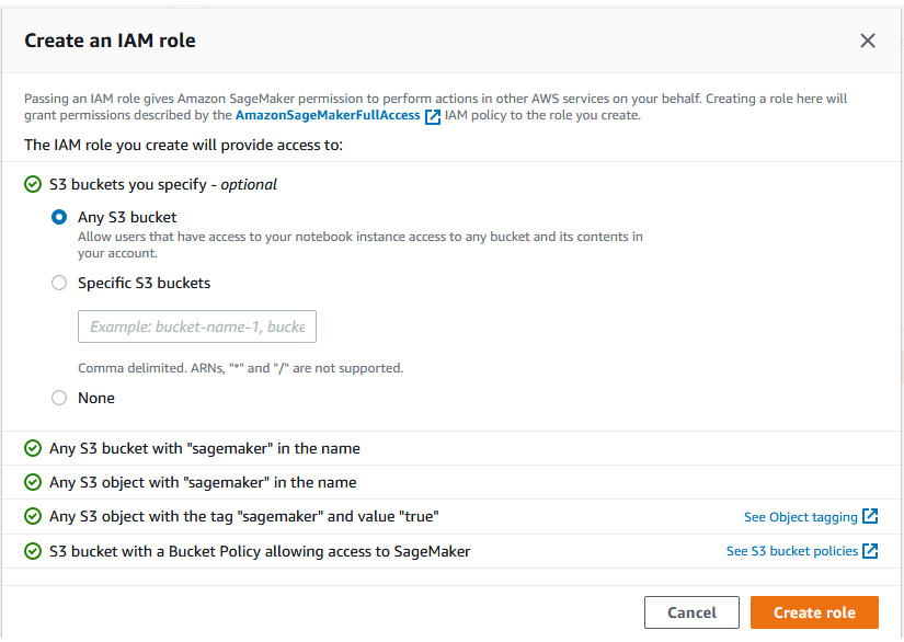
Figure 2.4 – Create an IAM role dialog

8. Click on the Create role button to close the dialog box and return to the Setup SageMaker Domain screen.
9. Click on the newly created IAM role to open the IAM console summary page dashboard.
10. Now click on the Add inline policy link, in the Permissions policies section, to open the Create policy screen.
11. Click the Import managed policy option, at the top right of the Create policy screen.
12. Once the Import managed policies dialog opens, check the radio button next to AdministratorAccess, and then click on the Import button.
13. On the Create policy screen, click on the Review policy button.
14. Once the Review policy screen opens, provide a name for the policy, such as AdminAccess-InlinePolicy, and then click the Create policy button.

    Note

    Providing administrator access to the SageMaker execution role is not a recommended practice in a production scenario. Since we will access various other AWS services throughout the hands-on examples within this book, we will use the administrator access policy to streamline service permissions.

15. Close the IAM console tab and go back to the SageMaker console.
16. Leave the rest of the Setup SageMaker Domain options as their defaults and click the Submit button.
17. If you are prompted to select a VPC and subnet, select any subnet in the default VPC and click the Save and continue button.

    Note

    If you are unfamiliar with what a VPC is, you can refer to the following AWS documentation (https://docs.aws.amazon.com/vpc/latest/userguide/what-is-amazon-vpc.html).

18. After a few minutes, the SageMaker Studio domain and user will be configured and, as shown in Figure 2.5, you should see the SageMaker domain:

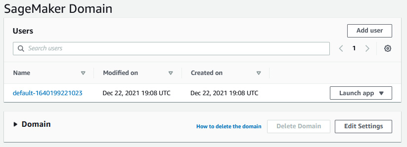
Figure 2.5 – Studio control panel

19. Click on the Launch app drop-down box next to the default name you created in step 5 and click Studio to launch the Studio IDE web interface.
20. Studio will take a few minutes to launch since this is the first time the Jupyter server is being initialized.

Now that we have the Studio UI online, we can start using Autopilot. But first, we need our raw data.

Preparing the experiment data

Autopilot treats every invocation of the ML process as an experiment and, as you will see, creating an experiment using Studio is simple and straightforward. However, before the experiment can be initiated, we need to provide the experiment with raw data.

Recall from Chapter 1, Getting Started with Automated Machine Learning on AWS, that the raw data was downloaded from the UCI repository. We have provided a copy of this data, along with the column names already added in the accompanying GitHub repository (https://github.com/PacktPublishing/Automated-Machine-Learning-on-AWS/blob/main/Chapter02/abalone_with_headers.csv). In order for any of the SageMaker modules to interact with data, the data needs to be uploaded to the AWS cloud and stored as an object, using the Amazon Simple Storage Service (S3).

Note

You can review the product website (https://aws.amazon.com/s3) if you are unfamiliar with what S3 is and how it works.

Use the following procedure to upload the raw data, for the Autopilot experiment, to S3:

1. Download the preceding file from the accompanying repository to your local machine.
2. To upload the file to Amazon S3, open the S3 console (https://s3.console.aws.amazon.com/s3) in a new web browser tab and then click the bucket name that starts with sagemaker-studio. This S3 bucket was automatically created for you when you used the QuickStart process to onboard to Studio.
3. As Figure 2.6 shows, the sagemaker-studio-… bucket is empty. To upload the raw data file to the bucket, click the Upload button to open the dialog shown in Figure 2.6:

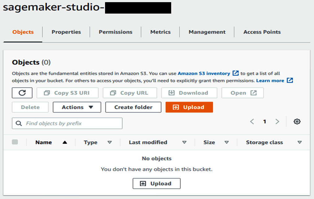
Figure 2.6 – SageMaker Studio bucket

4. On the Upload dialog screen, simply drag and drop the abalone_with_headers.csv file from its download location to the Upload dialog screen. Then click the Upload button, as shown in Figure 2.7:

Figure 2.7 – File upload

5. Once the file has been uploaded, click the Close button.

Now we have our data residing in AWS, we can use it to initiate the Autopilot experiment.

Starting the Autopilot experiment

Now that the data has been uploaded, we can use it to kick off the Autopilot experiment:

1. Using the Studio UI, click the SageMaker Components and registries icon on the left sidebar:

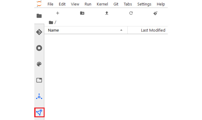
Figure 2.8 – SageMaker Component and registries icon

This will open the SageMaker resources navigation pane.

Tip

If you are unfamiliar with navigating the Studio UI, refer to the Amazon SageMaker Studio UI Overview in the AWS documentation (https://docs.aws.amazon.com/sagemaker/latest/dg/studio-ui.html).

2. From the drop-down menu, select Experiments and trials and then click the Create Autopilot Experiment button, as shown in Figure 2.9, to launch the Create experiment tab:

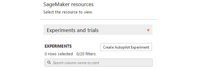
Figure 2.9 – Create Autopilot Experiment

3. The Create experiment tab enables you to set the key configuration parameters for the Autopilot experiment.
4. In the AUTOPILOT EXPERIMENT SETTINGS dialog, enter the following important settings for the experiment (all other settings can be left at their defaults):
   • Experiment name: This is the name of the experiment and it must be unique, in order to track lineage and the various assets created by Autopilot. For this example, enter abalone-v0 as the experiment name:

Figure 2.10 – Experiment name

Tip

In practice, it is a good idea to include the date and time the experiment was initiated or some other form of versioning information, as part of the experiment name. This way, the ML practitioner can easily track the experiment lineage as well as the various experiment assets and ensure these are distinguishable between multiple experiments. For example, if we were creating an experiment for the abalone dataset on July 1, 2021, we could name the experiment abalone-712021-v0.

• Input Data Location: This is the S3 bucket location that contains the raw dataset you uploaded in the previous section. Using the S3 bucket name dropdown, select the bucket that starts with sagemaker-studio. Under Dataset file name, select the abalone_with_headers.csv file that you previously uploaded:

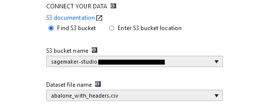
Figure 2.11 – Input data location

• Target Attribute Name: This is the name of the feature column, within the raw dataset, on which Autopilot will learn to make accurate predictions. In the Target drop-down box, select rings as the target attribute:

Figure 2.12 – Target attribute name

Note

The fact that the ML practitioner must supply a target label highlights a critical factor that must be taken into consideration when using Autopilot. Autopilot only supports supervised learning use cases. Basically, Autopilot will only try to fit supported models for regression and classification (binary and multi-class) problems.

• Output data location: The S3 bucket location for any artifacts that are produced by the experiment. From the S3 bucket name dropdown, select the bucket that starts with sagemaker-studio. Then, enter output for Dataset directory name to store the experiment output data:

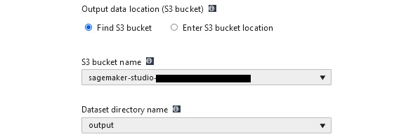
Figure 2.13 – Output data location

• Problem Type: This field specifies the type of ML problem to solve. As already noted, this can be a regression, binary classification, or multiclass classification problem. For this example, we will let Autopilot determine which of these problems we are trying to solve by selecting Auto from the drop-down box:

Figure 2.14 – Problem type

Tip

Some of the more experienced ML practitioners might be able to immediately determine the type of problem, based on the use case, and can therefore specify the Autopilot problem type. Should a novice ML practitioner not be able to deduce the type of ML problem, they should set this parameter to Auto, since Autopilot has the capability to determine the type of ML problem.

• Auto deploy: This option specifies whether to automatically deploy the best model as a production-ready, SageMaker-hosted endpoint. For this example, set the Auto deploy option to Off so as not to incur unnecessary AWS costs:

Figure 2.15 – Auto deploy

5. To start the automated experiment, click the Create Experiment button.

The experiment is now running and, as you can see, the process of creating a production-grade model using Autopilot is straightforward. However, you are probably wondering what's actually happening in the background, to produce this production-grade model. Let's take a behind-the-scenes look at what's actually going on in the experiment.

Running the Autopilot experiment

Once the experiment has been created, Autopilot will create the best possible candidate for production. The overall process will take approximately 2 hours to complete and the progress can be tracked in a Studio UI tab dedicated to the experiment. Figure 2.16 shows an example experiment tab:

Figure 2.16 – Experiment tab

As the experiment progresses, the various trails that make up the experiment will be displayed in the experiment tab, along with the trial that produces the best model and its overall evaluation score. Figure 2.17 shows an example of a completed experiment:

Figure 2.17 – Completed experiment

Once the experiment has been completed, you can right-click on the best model (or any of the other trials) and view the specific details. The following important details on the model are provided:

• The type of ML problem that Autopilot evaluated, based on the raw data
• The algorithm it used to address the assessed ML problem
• The metrics obtained from training the model and used to assess its performance
• The optimization parameters used to tune the model
• The S3 location for the various artifacts that were produced throughout the process
• An explainability report detailing the contribution of each feature, within the raw dataset, to the prediction
• The capability to deploy the model as a SageMaker hosted endpoint

So, by means of a simple process, all the heavy lifting tasks for data analysis, model building, training, evaluation, and tuning have been automated and managed by Autopilot, making it easy for the novice ML practitioner to overcome the two main challenges imposed by the ML process.

While this may suffice for an inexperienced application developer or novice ML practitioner to simply get a model into production, a more experienced ML practitioner may require more proof of why the particular model is the best and how it was produced. Figure 2.18 shows an overview of how Autopilot produces the best models:

Figure 2.18 – Overview of the AutoML process used by Autopilot

As you can see from Figure 2.18, there are six key tasks that Autopilot is automatically executing in the background:

1. Data Analysis
2. Candidate Generation
3. Feature Engineering
4. Candidate Tuning
5. Best Candidate
6. Candidate Deployment

Let's follow each step of the process in detail.

Data preprocessing

The first step of the ML process is to access the raw dataset and understand it, in order to clean it up and prepare it for model training. Autopilot does this automatically for us executing the data analysis and preprocessing step. Here, Autopilot leverages the SageMaker Processing module to statistically analyze the raw dataset and determine whether there are any missing values. Autopilot then shuffles and splits the data for model training and stores the output data in S3. Once the raw data has been preprocessed, it's ready for the model candidate generation step.

Should Autopilot encounter any missing values within the dataset, it will attempt to fill in the missing data using a number of different techniques. For example, for any missing categorical values, Autopilot will create a distinct unknown category feature. Alternatively, for any missing numeric values, Autopilot will try to impute the value using the mean or median of the feature column.

Generating AutoML candidates

The next step that Autopilot performs is to generate model candidates. In essence, each candidate is an AutoML pipeline definition that details the individual parts of a workflow that produces an optimized model candidate, or best model. Based on Autopilot's statistical understanding of the data, each candidate definition details the type of model to be trained and then, based on that model candidate, the data transformations necessary to engineer features that best suit the algorithm.

Depending on which problem type setting was specified when creating the experiment, Autopilot will select the appropriate algorithm from SageMaker's built-in estimators. In the case of the Abalone Calculator example, Auto was selected, and therefore, Autopilot deduces from analyzing the dataset that this is a regression problem, so it creates candidate definitions that each implement a variation of the Linear Learner Algorithm, XGBoost Algorithm, and a Multi-layer Perceptron deep learning algorithm. Each of these candidates has its own set of training and testing data, as well as the specific ranges of hyperparameters to tune on. Autopilot creates up to 10 candidate definitions.

Tip

For more information on Autopilot's supported algorithms, you can review the Model Support and Validation section of the AWS documentation (https://docs.aws.amazon.com/sagemaker/latest/dg/autopilot-model-support-validation.html).

Figure 2.18 highlights the outputs from the Candidate Generation step, two Jupyter notebooks:

• Data Exploration Notebooks: This notebook provides an overview of the data that was analyzed during the Data Analysis step and provides guidance for the ML practitioner to investigate further.
• Candidate Definition Notebooks: This notebook provides a detailed overview of the model candidates, recommended data processing for the candidate, and what hyperparameters should be tuned to optimize the candidate. The notebook even generates Python code cells, with the appropriate SageMaker SDK calls, to reproduce the candidate pipeline, thus giving the novice ML practitioner a how-to guide on reproducing a production-ready model.

If you recall from Chapter 1, Getting Started with Automated Machine Learning on AWS, one of the earmarks of an efficient AutoML process is the fact that the process must be repeatable. By providing candidate definition notebooks, not only does Autopilot provide a how-to guide for the ML practitioner but also allows them to build upon the process and create their own candidate pipelines.

Tip

Since AutoML technically only needs to be executed once, to get the best candidate for production deployment, these notebooks can be used as a foundation to further customize and develop the model.

Before these model candidates can be trained, the raw data must be formatted to suit the specific algorithm that the candidate pipeline will use. This process happens next.

Automated feature engineering

The next step of the AutoML process is the feature engineering stage. Here, Autopilot once again leverages the SageMaker Processing module to engineer these new features, specific to each model candidate. Autopilot then creates training and validation dataset variations that include these features and stores these on S3. Each candidate now has its own formatted training and testing dataset. Now the training process can begin.

Automated model tuning

At this stage of the process, Autopilot has the necessary components to train each of the candidate models. Unlike the typical ML process, where each candidate is trained, tuned, and evaluated, Autopilot leverages SageMaker's automatic model tuning module to execute the process in parallel.

As explained at the outset of this chapter, the hyperparameter optimization module uses Bayesian Search to find the best parameters for the model. However, Autopilot takes this one step further and leverages SageMaker's native capability to extend the tuning capability across multiple algorithms as well. In essence, Autopilot not only finds the best hyperparameters for an individual model candidate but the best hyperparameters when compared to all the other model candidates.

As already mentioned, Autopilot performs this process in parallel, training, tuning, and evaluating each model candidate with a subset of hyperparameters in order to get the best model candidate and associated hyperparameters for that subset, as a trial. The process is then repeated, constantly refining the hyperparameters, up to the default of 250 trials. This capability greatly reduces the overall time taken to produce an optimized model to a matter of hours as opposed to days or weeks when using a manual ML process.

The tuning process produces up to 250 candidate models. Let's review these candidate models next.

Candidate model selection

As Figure 2.17 highlights, the model that produces the best evaluation metric result is labeled Best.

The outputs from this step are the models and the associated artifacts for each trial and an explainability report. Autopilot uses another SageMaker module, called SageMaker Clarify, to produce this report.

Clarify helps ML practitioners understand how and why trained models make certain predictions, by quantifying the contribution that each feature of the dataset makes towards the model's overall prediction. This helps not only the ML practitioner but also the use case stakeholders, to understand how the model determines its predictions. Understanding why a model makes certain predictions promotes further trust in the model's capability to address the goals and requirements of the business use case.

Tip

For more information on the process that SageMaker Clarify uses to quantify feature attributions, you can refer to the Model Explainability page in the SageMaker documentation (https://docs.aws.amazon.com/sagemaker/latest/dg/clarify-model-explainability.html).

The experiment is now complete, so all that's left for the ML practitioner to do is deploy the best candidate into production.

Candidate model deployment

The best model can now be automatically, or manually, deployed as a SageMaker Hosted Endpoint. This means that the best candidate is now an API that can be programmatically called upon to provide predictions for the production application. However, simply deploying the model into production doesn't stop the ML process. The process is continuous and there are a number of tasks still to be performed after experimentation.

Post-experimentation tasks

In the previous chapter, we emphasized that the CRISP-DM methodology ends with the model being deployed into production, and we also highlighted that producing a production-ready model is not necessarily the conclusion of an ML practitioner's responsibilities.

The same concepts apply to the AutoML process. While Autopilot takes care of the various steps to generate a production-ready model, this is typically a one-time process for the specific use case and Autopilot concludes the experiment after the model has been deployed. On the other hand, the ML practitioner's obligations are ongoing since the production model needs to be continuously monitored to ensure that it does not drift from its intended purpose.

However, by providing all the output artifacts for each model candidate as well as the candidate notebooks, Autopilot lays a firm foundation for the novice ML practitioner to close the loop on the ML process and continuously optimize future production models, should the deployed model drift from its intended purpose.

Additionally, SageMaker hosted endpoints provide added functionality to assist with the process of continuously monitoring the production model for concept drift. For example, should the ML practitioner decide to manually deploy the best candidate model in the Studio UI, they can enable data capture when selecting the best candidate and clicking on the Deploy Model button. Figure 2.19 shows the options available before deploying the model using the Studio UI:

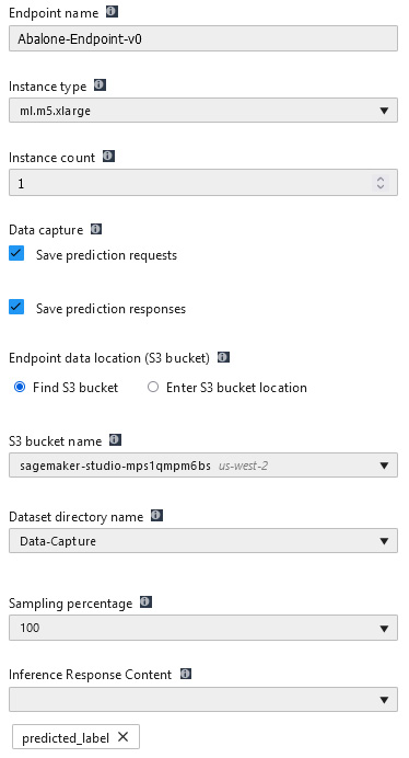
Figure 2.19 – Deployment options

Enabling the Data capture settings configures the endpoint to capture all incoming requests for prediction as well as the prediction responses from the deployed model. The captured data can be used by SageMaker's Model Monitor feature to monitor the production model in real time, continuously assessing its performance on unseen requests and looking for concept deviations.

Tip

For more information on the types of monitoring that SageMaker Model Monitor performs, you can refer to the SageMaker documentation (https://docs.aws.amazon.com/sagemaker/latest/dg/model-monitor.html).

From this example, you can see that by utilizing the Studio UI to create and manage an AutoML experiment (with Autopilot), a software developer or novice ML practitioner can easily produce a production-grade ML model with little to no experience and without writing any code.

However, some experienced ML practitioners may prefer documents and codify the experiment using a Jupyter notebook so that it is reproducible. In the next section, we will look at how to codify the AutoML experiment.

Using the SageMaker SDK to automate the ML experiment

In Chapter 1, Getting Started with Automated Machine Learning on AWS, you were provided with sample code to walk through the manual and iterative ML process. Since SageMaker is an AWS web service, we can also use code to interact with its various modules using the Python SDK for AWS, or boto3. More importantly, AWS also provides a dedicated Python SDK for SageMaker, called the SageMaker SDK.

In essence, the SageMaker SDK is a higher-level SDK that uses the underlying boto3 SDK with a focus on ML experimentation. For example, to deploy a model as a SageMaker hosted endpoint, an ML practitioner would have to use three different boto3 calls:

1. The ML practitioner must instantiate a trained model using the output artifact from a SageMaker training job. This is accomplished using the create_model() method from boto3's low-level SageMaker client, boto3.client("sagemaker").
2. Next, the ML practitioner must create a SageMaker hosted endpoint configuration, specifying the underlying computer resources and additional configuration settings for the endpoint. This is done using the create_endpoint_config() method from the SageMaker client.
3. Finally, the create_endpoint() method is used to deploy the trained model with the endpoint configuration settings.

Alternatively, the ML practitioner could accomplish the same objective by simply using the deploy() method on an already trained model, using the SageMaker SDK. The SageMaker SDK creates the underlying model, endpoint configuration, and automatically deploys the endpoint.

Using the SageMaker SDK makes ML experimentation much easier for the more experienced ML practitioner. In this next section, you will start familiarizing yourself with the SageMaker SDK by working through an example to codify the AutoML experiment.

Codifying the Autopilot experiment

In the same way that an ML practitioner uses a Jupyter notebook to execute a manual and interactive ML experiment, the Studio UI can also be used to accomplish these same tasks. The Studio IDE provides basic Jupyter Notebook functionality and comes pre-installed with all the Python libraries and deep learning frameworks an ML practitioner might use, in the form of AWS engineered Jupyter kernels.

Tip

If you are unfamiliar with the concept of a Jupyter Kernel and how they are used, you can refer to the Jupyter documentation website (https://jupyter-notebook-beginner-guide.readthedocs.io/en/latest/what_is_jupyter.html#kernel).

Let's see how this works by using a Jupyter notebook to execute the following sample code:

1. Using the Studio UI menu bar, select File | New | Notebook to open a blank Jupyter notebook.
2. As Figure 2.20 shows, you will be prompted to select an appropriate kernel from the selection of pre-installed kernels. From the drop-down list, select Python 3 (Data Science):

Figure 2.20 – Jupyter kernel selection

3. In the background, Studio will initialize a dedicated compute environment, called a KernelGateway. This compute environment, with 2 x vCPUs and 4 GB of RAM, is in essence the engine that executes the various code cells within the Jupyter notebook. It may take 2–3 minutes to initialize this compute environment.
4. Once the Kernel has started, we can create the first code cell, where we import the SageMaker SDK and configure the SageMaker session by initializing the Session() class. The Session() class is a wrapper for the underlying boto3 client, which governs all interactions with the SageMaker API, as well as other necessary AWS services:

   import sagemaker

   import pandas as pd

   role = sagemaker.get_execution_role()

   session = sagemaker.session.Session()

   Tip

   If you are new to navigating through a Jupyter notebook, to execute a code cell, you can either click on the run icon or press the Shift + Enter keys on the highlighted cell.

5. Next, we can use the same code we used in Chapter 1, Getting Started with Automated Machine Learning on AWS, to download the raw abalone dataset from the UCI repository, add the necessary column headings, and then save the file as a CSV file called abalone_with_headers.csv:

   column_names = ["sex", "length", "diameter", "height", "whole_weight", "shucked_weight", "viscera_weight", "shell_weight", "rings"]

   abalone_data = pd.read_csv("http://archive.ics.uci.edu/ml/machine-learning-databases/abalone/abalone.data", names=column_names)

   abalone_data.to_csv("abalone_with_headers.csv", index=False)

6. Now, we can configure the Autopilot experiment, using the AutoML() class and using the following example code to create a variable called automl_job:

   from sagemaker.automl.automl import AutoML

   automl_job = AutoML(

       role=role,

       target_attribute_name="rings",

       output_path=f"s3://{session.default_bucket()}/abalone-v1/output",

       base_job_name="abalone",

       sagemaker_session=session,

       max_candidates=250

   )

This variable will interact with the Autopilot experiment. As we did in the previous section, we also supply the important parameters for the experiment:

• target_attribute_name: The name of the feature column within the raw dataset on which Autopilot will learn to make accurate predictions. Recall that this is the rings attribute.
• output_path: Where any artifacts that are produced by the experiment are stored in S3. In the previous example, we used the default S3 bucket that was created during the Studio onboarding process. However, in this example, we will use the default bucket provided by the SageMaker Session() class.
• base_job_name or the name of the Autopilot experiment. Since we already have a version zero, we will name this experiment abalone-v1.

  Note

  No versioning information has been supplied to the base_job_name parameter. This is because the SDK automatically binds the current date and time for versioning.

7. To initiate the Autopilot experiment, we call the fit() method on the automl_job variable, supplying it with the S3 location of the raw training data. We also call the SageMaker session upload() method, as a parameter to the fit() method since the data has not yet been uploaded to the default S3 bucket. The upload() method takes the bucket name (the SageMaker default bucket) and the prefix (the folder structure) as parameters to automatically upload the raw data to S3. The following code shows an example of how to correctly call the fit() method:

   automl_job.fit(inputs=session.upload_data("abalone_with_headers.csv", bucket=session.default_bucket(), key_prefix="abalone-v1/input"), wait=False)

At this point, the Autopilot experiment has been started and, as was shown in the previous section, the experiment can be monitored using the Experiments and trials dropdown in the SageMaker Components and registries section of the Studio UI. Right-click on the current Autopilot experiment and select Describe AutoML Job.

Alternatively, we can use the describe_auto_ml_job() method on the automl_job variable to programmatically get the current overview of the Autopilot job.

Note

Make a note of the automatically generated versioning information that the SDK appends to the job name. As you will see later, this job name is used to programmatically explore the experiment as well as to clean it up.

To make the experiment reproducible, some ML practitioners might want to include a visual comparison of the resultant models. Now that the AutoML experiment is underway, we can wait for it to complete to see how the models compare and explore how the SageMaker SDK enables experiment analysis.

Analyzing the Autopilot experiment with code

Once the Autopilot experiment has been completed, we can use the analytics() class from the SageMaker SDK to programmatically explore the various model candidates (or trials) to compare candidate evaluation results, in the same way we used the Studio UI in the previous section.

Let's analyze the experiment by using the same Jupyter notebook to execute the following sample code:

1. The first thing we need to do is load the ExperimentAnalytics() class from the SageMaker SDK to get the trial component data and make them available for analysis. By providing the name of the Autopilot experiment, the following sample code instantiates the automl_experiment variable, whereby we can interact with the experiment results. Additionally, since the SageMaker SDK automatically generates the versioning information for the experiment name, we can once again use the describe_auto_ml_job() method to find the AutoMLJobName:

   from sagemaker.analytics import ExperimentAnalytics

   automl_experiment = ExperimentAnalytics(

       sagemaker_session=session,

       experiment_name="{}-aws-auto-ml-job".format(automl_job.describe_auto_ml_job()["AutoMLJobName"])

   )

2. Next, the following sample code converts the returned experiment analytics object into a pandas DataFrame for easier analysis:

   df = automl_experiment.dataframe()

3. An example of such analysis might be to visually compare the evaluation results of the top five trials. The following sample code filters the DataFrame by the latest evaluation accuracy metrics, validation:accuracy – Last and train:accuracy - Last, on both the training dataset and validation dataset respectively, and then sorts these values in ascending order:

   df = df.filter(["TrialComponentName","validation:accuracy - Last", "train:accuracy - Last"])

   df = df.sort_values(by="validation:accuracy - Last", ascending=False)[:5]

   df

Figure 2.21 shows what an example of this DataFrame would look like:

Figure 2.21 – Sample top 5 trials

4. We can further visualize the comparison using a plot by means of the matplotlib library:

   import matplotlib.pyplot as plt

   %matplotlib inline

   legend_colors = ["r", "b", "g", "c", "m"]

   ig, ax = plt.subplots(figsize=(15, 10))

   legend = []

   i = 0

   for column, value in df.iterrows():

       ax.plot(value["train:accuracy - Last"], value["validation:accuracy - Last"], "o", c=legend_colors[i], label=value.TrialComponentName)

       i +=1

   plt.title("Training vs.Testing Accuracy", fontweight="bold", fontsize=14)

   plt.ylabel("validation:accuracy - Last", fontweight="bold", fontsize=14)

   plt.xlabel("train:accuracy - Last", fontweight="bold", fontsize=14)

   plt.grid()

   plt.legend()

   plt.show()

Figure 2.22 shows an example of the resultant plot:

Figure 2.22 – Plot of the top 5 trials

Using the ExperimentAnalytics() class is a great way to interact with the various trials of the experiment, however, you want to simply see which trial produces the best candidate. By calling the best_candidate() method on the Autopilot job, we can not only see which trial produced the best candidate, but also the value of the candidate's final evaluation metric. For example, the following sample code produces the name of the best candidate:

automl_job.best_candidate()["CandidateName"]

When executing the preceding code in the Jupyter notebook, you will see an output similar to the following:

'abalone-2021-07-05-17-07-15-99Qg-240-9bfa065e'

Likewise, the following sample code can be executed in an additional notebook cell to see the best candidate's evaluation metrics:

automl_job.best_candidate()["FinalAutoMLJobObjectiveMetric"]

The results of this code will be similar to the following:

{'MetricName': 'validation:accuracy', 'Value': 0.292638897895813}

Additionally, just as with the example in the previous section, you can also programmatically view the S3 location of the Data Exploration notebook, Candidate Definition notebook, and the Explainability Report.

The following code samples can be used to get this information:

• Data Exploration Notebook:

  automl_job.describe_auto_ml_job()["AutoMLJobArtifacts"]["DataExplorationNotebookLocation"]

• Candidate Definition Notebook:

  automl_job.describe_auto_ml_job()["AutoMLJobArtifacts"]["CandidateDefinitionNotebookLocation"]

• Explainability Report:

  automl_job.describe_auto_ml_job()["BestCandidate"]["CandidateProperties"]["CandidateArtifactLocations"]["Explainability"]

Using the analytics() class of the SageMaker SDK and, the various Autopilot output artifacts has allowed us to gain further insight into the experiment. All that's left is to deploy the production model.

Deploying the best candidate

The last part of the AutoML process is to deploy the best model as a production API, as a SageMaker hosted endpoint. To provide for this functionality, the SageMaker SDK once again provides a simple method, called deploy().

Note

Hosting the best model on SageMaker will incur AWS usage costs that exceed what is provided by the free tier.

Let's run the following code to deploy the best model:

automl_job.deploy(

    initial_instance_count=1,

    instance_type="ml.m5.xlarge",

    candidate=automl_job.best_candidate(),

    sagemaker_session=session,

    endpoint_name="-".join(automl_job.best_candidate()["CandidateName"].split("-")[0:7])

)

As was the case with the fit() method, simply calling the deploy() method and providing some important parameters will create a hosted endpoint:

• We need to supply the type of computer resources to process inference requests by supplying the instance_type parameter. In this case, we selected the ml.m5.xlarge instance.
• We then need to specify the number of instances. In this case, we are specifying one instance.
• We can either deploy a specific candidate, by providing the Python dictionary for the specific candidate or, if no candidate is provided, the deploy() method will automatically use the best candidate.
• Lastly, we need to provide the unique name for the endpoint. This name will be used to provide model predictions to the business application.

  Tip

  When naming the endpoint, it is a good practice to use the versioning information supplied to the experiment in order to tie specific endpoints to the experiment that produced them. From the preceding sample Python code, you can see that we derived endpoint_name by using the best_candidate() method and filtering the response by "CandidateName".

Once the code cell is executed, SageMaker will automatically deploy the best model on the specific compute resources and make the endpoint API available for inference requests, thus completing the experiment.

Note

Unlike the preceding example, where the Studio UI is used to deploy the model, using the AutoML() class from the SageMaker SDK does not include the ability to enable data capture when deploying a model. Recall that the ability to capture both inference requests and inference responses enables the ML practitioner to use this data to continuously monitor a production model. It is recommended that you use the SageMaker SDK's Model() class to deploy the model. This class allows you to specify the data_capture_config parameter, should you wish to close the loop on continuous model monitoring. You can learn more about the Model() class in the SageMaker SDK documentation (https://sagemaker.readthedocs.io/en/stable/api/inference/model.html#sagemaker.model.Model.deploy).

As was the case with the typical ML process, highlighted in Chapter 1, Getting Started with Automated Machine Learning on AWS, the deployed model can now be handed over to the application development owners for them to test and integrate the model into the production application. However, since the intended purpose of this example was to simply demonstrate how to make the required SageMaker SDK calls to execute the AutoML experiment, we are not going to use the model to test inferences. Instead, the next section demonstrates how to delete the endpoint.

Cleaning up

To avoid unnecessary AWS usage costs, you should delete the SageMaker hosted endpoint. This can be accomplished by using the AWS SageMaker console (https://console.aws.amazon.com/sagemaker) or by using the AWS CLI. Run the following commands in the Jupyter notebook to clean up the deployment:

1. Using the AWS CLI, delete the SageMaker hosted endpoint:

   !aws sagemaker delete-endpoint --endpoint-name {"-".join(automl_job.best_candidate()["CandidateName"].split("-")[0:7])}

2. Then use the AWS CLI to also delete the endpoint configuration:

   !aws sagemaker delete-endpoint-config --endpoint-config-name {"-".join(automl_job.best_candidate()["CandidateName"].split("-")[0:7])}

   Tip

   If you wish to further clean up the various trials from the experiment, you can refer to the Clean Up section of the SageMaker documentation (https://docs.aws.amazon.com/sagemaker/latest/dg/experiments-cleanup.html).

From the perspective of automating the ML process, you should now be acquainted with how the Autopilot module can be used to realize an AutoML methodology, and how the SageMaker SDK can be used to create a codified and documented AutoML experiment.

Summary

This chapter introduced you to some of AWS's AI and ML capabilities, specifically Amazon SageMaker's. You saw how to interact with the service via the SageMaker Studio UI and the SageMaker SDK. Using hands-on examples, you learned how Autopilot's implementation of the AutoML methodology addresses not only the two challenges imposed by the typical ML process but also the overall criteria for automation. Particularly, how using Autopilot ensures that the ML process is reliable and streamlined. The only task required to be done by the ML practitioner is to upload the raw data to Amazon S3.

This chapter also highlights an important aspect of the AutoML methodology. While the AutoML process is repeatable in the sense that it will always produce an optimized model, once you have the model in production, there is no real need to recreate it, unless, of course, the business use case changes. Nevertheless, Autopilot creates a solid foundation to help an ML practitioner continuously optimize the production model, by providing Candidate Notebooks, model Explainability Reports, and enabling Data Capture to monitor the model for concept drift. So, using the AutoML methodology is a great way for ML practitioners to automate their initial ML experiments.

Worth noting is a drawback of Autopilot's implementation of the AutoML methodology. Autopilot only supports Supervised Learning use cases – ones that use Regression or Classification models.

In the next chapter, you will learn how to apply the AutoML methodology to more complicated ML use cases that require advanced deep learning models, using the AutoGluon package.