
Optimization is more than finding the best simulation results. It is itself a complex and evolving field that, subject to certain information constraints, allows data scientists, statisticians, engineers, and traders alike to perform reality checks on modeling results. We will discuss common ideological pitfalls and how to avoid them. We will talk about cross validation and its specific application to time series, and we will use our simulator from Chapter 7 to project trading performance with confidence and validity.
We will discuss the best optimization methods and performance metrics. Our simulator takes a considerable amount of time to run, so it is in our best interest to condense parameters and minimize calls to the function within an optimizer.
Cross Validation in Time Series
In Chapter 7, we built a simulator. The simulator tells us how a given strategy with certain account constraints performs over a period of time. Developers can manually test and reconfigure strategies to learn which strategies and configurations perform best over a certain period of time. Developers will be tempted to assume that a configuration that performs well in one period will perform similarly in another. As a basic principle of statistics, we know that good performance in the past does not guarantee good performance in the future. The vast majority of people will avoid this ideological pitfall.
There are less obvious ideological pitfalls we need to avoid. A developer may feel some sense of accomplishment when he discovers a strategy and configuration that performs well over a long period of time. Naturally, there is reason to get excited about a strategy that makes solid returns over years or decades and avoids catastrophic losses during recessions. Unfortunately, this is a substantial ideological pitfall.
The developer has tinkered with the strategy and parameters to optimize performance over a long period of time. He assumes that this strategy will perform well in the future because it weathered many business cycles and made consistent gains. He is excited to put the strategy into production and start generating profits, but important logistics questions remain. How will he determine the best strategy a year from now? Will he keep using the current strategy? Or will he repeat the process of optimizing over all available data and use the best new strategy in the following year? Important projection questions remain. If the strategy made 30 percent in 2016, how much can the developer expect to make 2017?
Any performance projections of a strategy optimized in this manner are invalid because of the use of information in the future to adjust parameters in the past. In classical statistics, optimization in this manner is called curve fittingand is solved by cross validation.
In statistics, the concepts of tests and models correspond to the concepts of simulations and strategies in trading. The motivating idea behind cross validation is that test results are not valid unless there is (at minimum) a weakly deterministic process for arriving at the parameterization of the model using information outside and independent of the test data set .
In trading terms, simulation performance is not valid unless there is (at minimum) a weakly deterministic process for arriving at the parameterization of the trading strategy using only data available before data in the test data set.
A weakly deterministic process is one that relies on strictly deterministic processes and constrained randomness. A strictly deterministic process is a deliberate and repeatable functional mapping of one set of information to another. Constrained randomness is the generation of random numbers per a strictly deterministic probability distribution. The inclusion of weak determinism in addition to strict determinism exists to allow optimization procedures to declare search points and initial values at random.
Notice in our definition how “outside and independent” in statistics terms equates to “available before” in trading terms. This is a translation from the more general statistical definition of cross validation to the application-specific time-series definition. In most statistical applications, observations are assumed independent, so we can separate training and testing data by randomly sampling observations. In time series, if we want to simulate performance starting at time t, all data before t is our training data and all data after t is our testing data.
In short, simulation results for data occurring any time after t are trivial acts of curve fitting unless they use only information both occurring and available before t to determine the strategy. To generate performance simulations for the duration of our data, we will move through time, generating a given year’s performance simulation with a strategy determined by data available prior to it. This will necessarily exclude the performance simulation for the first year of our data, the year 2000, and include everything up to the present.
Numerical vs. Analytical Optimization
In general, the goal of an optimization problem for objective function ![]()
is to find the parameter vector θ such that
![]()
Ultimately, we may find the actual value of θ, or we might find an estimate ![]() because of natural constraints of the problem. We touched on the difference between analytical and numerical optimization in the introduction of this text. We will delineate further here.
because of natural constraints of the problem. We touched on the difference between analytical and numerical optimization in the introduction of this text. We will delineate further here.
In analytical optimization, we know the form and gradient of the objective function. Note that a gradient is a vector of derivatives in each dimension of the candidate parameter vector. To find the minimum of a function in analytical optimization, we solve for the points where the derivative is equal to zero and test them, keeping the arguments of the minimum value as the global minimum of the function. In almost every case, analytical optimization will find θ rather than ![]() . Analytical optimization is a problem commonly found in calculus and other advanced mathematics that is seldom seen again by practitioners in data science, statistics, and algorithmic trading.
. Analytical optimization is a problem commonly found in calculus and other advanced mathematics that is seldom seen again by practitioners in data science, statistics, and algorithmic trading.
Numerical optimization involves algorithmically searching for the minimum of a function with a known form but an unknown gradient. Claiming to know the form of the objective function is a mathematical technicality. We may know how to compute the objective function but find it too computationally expensive to examine its form comprehensively. We not only aim to find the minimum of a function with an undefined gradient but minimize the steps and time taken to find a reasonable estimate for a minimum.
We will only be dealing with numerical optimization in this text. The output of our objective function is a performance metric computed from the results of a simulation, and our simulations are very computationally expensive to run. We will cover a handful of optimization algorithms including Exhaustive, Genetic, Pattern Search, Nelder-Mead, and BFGS. Numerous functions and packages exist to run these algorithms given data and an objective function, but they typically assume near-instantaneous computation of the objective function and strictly continuous inputs. There is a clear necessity to program our own optimizers and adapt them to handle common problems and constraints of trading strategy optimization .
Note that we seek the minimum as opposed to the maximum of the objective function purely as convention. Most performance metrics in finance are designed to be maximized, so we minimize the negative of the performance metric in practice.
Numerical Optimization Overview
We will outline major concepts in numerical optimization and explain their uses.
Gradient optimizationinvolves approximating the gradient of the objective function with respect to its parameters to point the algorithm in the direction of a minimum value. These procedures perform best finding the minima of smooth functions with a medium to large number of parameters (ten or more). The algorithm generally takes steps in the parameter space proportional to the negative gradient in search of minima. Gradient optimization requires the objective function be relatively smooth. Substantial research efforts have sought to generalize gradient optimization to work with nonsmooth objective functions.
While it is possible to implement gradient procedures in trading strategy optimization, we will generally avoid them. Sophisticated gradient optimization algorithms are capable of efficiently locating minima of nonsmooth objective functions, but our objective function has the added challenge of taking integer parameters. Search methods are typically designed to find the minima of objective functions with continuous inputs, so integer inputs must be rounded after declaration to give the objective function a real-valued domain. This is a problem for gradient optimization because the objective function becomes stepwise with respect to integer-valued parameters. Gradients are computed to estimate the magnitude of parameter changes required to find the minimum. Numerical gradient estimates throw unwieldy and misleading values in stepwise functions because the gradient is technically undefined at every step. If we are rounding integer inputs before simulation, the true gradient is undefined at every point x+0.5 where x is any integer. Particularly unwieldy and misleading behavior occurs when calculating the gradient near or within steps, leading to unrealistically large or zero-valued gradients, respectively. Figure 8-1 illustrates this phenomenon for a one-dimensional parameter vector θ and the objective function ![]() .
.

Figure 8-1. Misleading gradient estimation in stepwise objective functions
We will avoid gradient search methods in favor of direct search methods . Direct search methods use searching algorithms to iteratively discover minima in the objective function. Direct search methods typically take an intuitive search procedure in a one- or two-dimensional parameter space and generalize them to n-dimensional parameter vectors. We will cover exhaustive search, generalized pattern search, and Nelder-Mead optimization. We will make preparations to run these algorithms in the next sections .
Parameter Transform for Unbounded Search Algorithms
The generalized pattern search and Nelder-Mead algorithms
assume continuous real-valued parameters on the domain of ![]() . We will take the logistic transform of the parameters when optimizing with these algorithms. Even in algorithms
that do not strictly require continuous unbounded inputs, transforming the parameters improves search robustness in general. Where x represents the input to the logistic function and p represents the logistic transform,
. We will take the logistic transform of the parameters when optimizing with these algorithms. Even in algorithms
that do not strictly require continuous unbounded inputs, transforming the parameters improves search robustness in general. Where x represents the input to the logistic function and p represents the logistic transform,

with the inverse

The output of the logistic function is bounded by (0,1). In practice, the optimizer will generate candidate vectors that are continuous on the domain ![]() . The purpose of the logistic transform is clearer from the manner in which we compute inputs into the simulator. Where θ
sim
is the candidate parameter vector of logically bounded inputs to the simulator, θ
min
is a vector of logical minima of the parameter vector, θ
max
is a vector of logical maxima of the parameter vector, and θ
opt
is the unbounded candidate vector generated by the optimization algorithm that exists on the domain
. The purpose of the logistic transform is clearer from the manner in which we compute inputs into the simulator. Where θ
sim
is the candidate parameter vector of logically bounded inputs to the simulator, θ
min
is a vector of logical minima of the parameter vector, θ
max
is a vector of logical maxima of the parameter vector, and θ
opt
is the unbounded candidate vector generated by the optimization algorithm that exists on the domain
![]() ,
,

This process maps the unbounded candidate vectors generated by optimizers to logically bounded domains specific to each parameter.
Declaring an Evaluator
Optimization algorithms are fairly plug-and-play given a compact evaluator function. An optimization algorithm needs to be able to evaluate the objective function given any valid candidate parameter vector. For our use case, we will declare an evaluator that takes a named parameter vector, transforms the inputs based on rectangular bounds (two constant named vectors) on the parameter vector, subsets our data for a given year, and returns a performance metric for the strategy.
The evaluator function , declared in Listing 8-1, will look sloppier than much of the code we have written up to this point. Any given evaluator function is not part of our code base, but it is a flexible outline of a specific strategy of interest. This function and declaration of inputs to the simulator, which will look strikingly similar, are the most fluid pieces of code presented in this text. They will be changed frequently while researching strategies.
Note:
The code for generating inputs to the long-only MACD has been optimized for speed within the evaluator. It does not match Listing 7-2. In this case, it was found that the runmean() function from the caTools package computes means faster than mcTimeSeries() because of internal algorithmic improvements. This sacrifices the ability to fine-tune NA-handling at the indicator level, but this is not an issue given the structure of our stock data as established in this text. Users with alternate data containing periodic or regular NA values should explore the ability of mcTimeSeries() and rollapply() to handle NA values at the indicator level.
Listing 8-1: Pseudocode
If requested, transform unbounded parameters to their original domains bounded between minVal and maxVal. This allows optimizers that require continuous unbounded inputs to communicate with our simulator that requires bounded and often integer-only values. If transformOnly = TRUE is specified, exit the function by returning the bounded parameters after transformation. This is a helpful shortcut for transforming unbounded parameters back into their practical domains without going through the lengthy simulation step.
Regardless of whether the supplied parameters underwent transformation in the first step, this step enforces numeric type and bounding rules as to not break the simulator. For example, we enforce that n1 is an integer greater than or equal to 2. Then we enforce that n2 is an integer greater than or equal to both n1 and 3. This code should be modified as new strategies are built into the evaluator. Incorrect bounding conditions during optimization is a large source of run-time errors .
We subset the data according to the argument y. This can be a range of years or a single year. The simulator will run over the range of years supplied.
The subset requires elements of the DATA object according to the previous step.
Compute the ENTRY, EXIT, and FAVOR matrix according to the strategy specified. This and step 2 are the most variable sections of code. They will change often as you research and develop new strategies.
Simulate the strategy and store the results in a list. If account parameters are passed to the evaluator, supply them to the simulator.
Compute the performance metric and return it. By default, we have supplied the High-Frequency Sharpe Ratio. This will change frequently as users explore new performance metrics. Return the negative of the performance metric if requested. Return the data from simulation rather than the performance metric if requested.
Listing 8-1: Explanation of Inputs and User Guide
PARAM is a named vector of inputs. These can be bounded according to minVal and maxVal or unbounded on the domain
 depending on the value of transform. PARAM must have names matching minVal and maxVal if they are supplied.
minVal and maxVal are named vectors of logical bounds on the values of parameters inputted to the strategy. They need to be supplied if transform or transformOnly is set to TRUE.
y is a single number, pair of numbers, or range of numbers corresponding to the years to evaluate over. y = 2016 will evaluate performance in 2016. y = 2011:2016 and y = c(2011,2016) will both evaluate performance from 2011 up to and through 2016.
transform specifies if PARAM is supplied as unbounded parameters subject to our domain transformation based on the logistic transform. If transform = TRUE, minVal and maxVal are required inputs. An example of PARAM input when transform = TRUE could be c(n1 = -0.23, nFact = 3.6, nSharpe = -2.5, shThresh = 3.1). An example of PARAM input with transform = FALSE could be c(n1 = 21, nFact = 3, nSharpe = 43, shThresh = 0.80).
verbose is the same as in Listing 7-1. This parameter is passed to the simulator if the user desires run-time diagnostics .
negative specified whether to return the negative value of the performance metric. This assumes that all performance metrics are coded such that greater values correspond to a better assessment of performance. This is useful for extending the evaluator to algorithms that perform minimization as opposed to algorithms that perform maximization.
transformOnly is set to TRUE if the user desires to use the evaluator as a shortcut to transform to unbounded parameters back to their logically bounded domains. It simply performs the transformation and halts the function early to return the logically bounded parameters.
returnData is set to TRUE if the user desires to bypass computation of the performance metric and return the list of account variables normally output from the simulator.
accountParams is set if the user desires to pass positions and cash data of the account across evaluations. This will come into play in Listing 8-6 when we cross validate using the optimization algorithms discussed in the chapter. The list provided to this argument must contain the final row of P, the final row of p, and the final element of C as defined in the Listing 7-1 pseudo-code and as seen in the output of Listing 7-1. See Listing 8-6 for an implementation example.
Listing 8-1. Declari ng the Evaluator Function
y <- 2014minVal <- c(n1 = 1, nFact = 1, nSharpe = 1, shThresh = .01)maxVal <- c(n1 = 150, nFact = 5, nSharpe = 200, shThresh = .99)PARAM <- c(n1 = -2, nFact = -2, nSharpe = -2, shThresh = 0)# Declare entry function for use inside evaluatorentryfunc <- function(v, shThresh){cols <- ncol(v)/2as.numeric(v[1,1:cols] <= 0 &v[2,1:cols] > 0 &v[2,(cols+1):(2*cols)] >quantile(v[2,(cols+1):(2*cols)],shThresh, na.rm = TRUE))}evaluate <- function(PARAM, minVal = NA, maxVal = NA, y = 2014,transform = FALSE, verbose = FALSE,negative = FALSE, transformOnly = FALSE,returnData = FALSE, accountParams = NULL){# Step 1# Convert and declare parameters if they exist on unbounded (-inf,inf) domainif( transform | transformOnly ){PARAM <- minVal +(maxVal - minVal) * unlist(lapply( PARAM, function(v) (1 + exp(-v))^(-1) ))if( transformOnly ){return(PARAM)}}# Step 2# Declare n1 as itself, n2 as a multiple of n1 defined by nFact,# and declare the length and threshold in sharpe ratio for FAVOR.# This section should handle rounding and logical bounding# in movingn1 <- max(round(PARAM[["n1"]]), 2)n2 <- max(round(PARAM[["nFact"]] * PARAM[["n1"]]), 3, n1+1)nSharpe <- max(round(PARAM[["nSharpe"]]), 2)shThresh <- max(0, min(PARAM[["shThresh"]], .99))maxLookback <- max(n1, n2, nSharpe) + 1# Step 3# Subset data according to range of years yperiod <-index(DATA[["Close"]]) >= strptime(paste0("01-01-", y[1]), "%d-%m-%Y") &index(DATA[["Close"]]) < strptime(paste0("01-01-", y[length(y)]+1), "%d-%m-%Y")period <- period |((1:nrow(DATA[["Close"]]) > (which(period)[1] - maxLookback)) &(1:nrow(DATA[["Close"]]) <= (which(period)[sum(period)]) + 1))# Step 4CLOSE <- DATA[["Close"]][period,]OPEN <- DATA[["Open"]][period,]SUBRETURN <- RETURN[period,]# Step 5# Compute inputs for long-only MACD as in Listing 7.2# Code is optimized for speed using functions from caTools and zoorequire(caTools)INDIC <- zoo(runmean(CLOSE, n1, endrule = "NA", align = "right") -runmean(CLOSE, n2, endrule = "NA", align = "right"),order.by = index(CLOSE))names(INDIC) <- names(CLOSE)RMEAN <- zoo(runmean(SUBRETURN, n1, endrule = "NA", align = "right"),order.by = index(SUBRETURN))FAVOR <- RMEAN / runmean( (SUBRETURN - RMEAN)^2, nSharpe,endrule = "NA", align = "right" )names(FAVOR) <- names(CLOSE)ENTRY <- rollapply(cbind(INDIC, FAVOR),FUN = function(v) entryfunc(v, shThresh),width = 2,fill = NA,align = "right",by.column = FALSE)names(ENTRY) <- names(CLOSE)EXIT <- zoo(matrix(0, ncol=ncol(CLOSE), nrow=nrow(CLOSE)),order.by = index(CLOSE))names(EXIT) <- names(CLOSE)# Step 6# Max shares to holdK <- 10# Simulate and store resultsif( is.null(accountParams) ){RESULTS <- simulate(OPEN, CLOSE,ENTRY, EXIT, FAVOR,maxLookback, K, 100000,0.001, 0.01, 3.5, 0,verbose, 0)} else {RESULTS <- simulate(OPEN, CLOSE,ENTRY, EXIT, FAVOR,maxLookback, K, accountParams[["C"]],0.001, 0.01, 3.5, 0,verbose, 0,initP = accountParams[["P"]], initp = accountParams[["p"]])}# Step 7if(!returnData){# Compute and return sharpe ratiov <- RESULTS[["equity"]]returns <- ( v[-1] / v[-length(v)] ) - 1out <- mean(returns, na.rm = T) / sd(returns, na.rm = T)if(!is.nan(out)){if( negative ){return( -out )} else {return( out )}} else {return(0)}} else {return(RESULTS)}}# To test value of objective functionobjective <- evaluate(PARAM, minVal, maxVal, y)
Exhaustive Search Optimization
It is wise to start your research on a new strategy with a wide-spanning exhaustive search. Exhaustive searches involve scanning an n-dimensional grid of parameters, where n is the number of parameters tested. Exhaustive testing is computationally expensive. If testing k
i
points for each parameter ![]() , the number of calls to the
evaluate() function
required to complete the optimization is
, the number of calls to the
evaluate() function
required to complete the optimization is
![]()
Exhaustive searches are helpful because they allow us to view surface plots of the objective function, informing more detailed exhaustive searches or initial values for other search methods. Listing 8-2 performs an exhaustive search by declaring every possible combination of the test points in the OPTIM data frame. Throughout this chapter, the OPTIM data frame will make a point of storing the inputs and results of every call to the evaluate function made by an algorithm, even when the algorithm does not call for or depend on this data.
Listing 8-2 includes a simple clock for estimating time to completion. It assumes the average completion time is constant throughout the optimization process, which is not necessarily true when parameters increase the maximum lookback and computational complexity as the search progresses. Nonetheless, it will give a rough estimate of time to completion for an optimization. Careless declaration of bounds and step sizes can initialize an optimization process that takes weeks or years.
Notice in Listing 8-2 that we declare equal lower and upper bounds on nFact and nSharpe. This is intentional in order to declare these values in the optimization but prevent the search procedure from scanning through different values of nFact and nSharpe.
We will declare transform = FALSE in our evaluator function to let it know we are not giving it transformed inputs. In Listing 8-2, we optimize with constant step size. You may want to specify transform = TRUE to test with a nonconstant step size in an unbounded parameter space. You can step into the beginning of this code and replace the elements of the POINTS list with any desired sequence of test points without disrupting the rest of the code.
Listing 8-2. Exhaustive Optimization
# Declare bounds and step size for optimizationlowerBound <- c(n1 = 5, nFact = 3, nSharpe = 22, shThresh = 0.05)upperBound <- c(n1 = 80, nFact = 3, nSharpe = 22, shThresh = 0.95)stepSize <- c(n1 = 5, nFact = 1, nSharpe = 1, shThresh = 0.05)pnames <- names(stepSize)np <- length(pnames)# Declare list of all test pointsPOINTS <- list()for( p in pnames ){POINTS[[p]] <- seq(lowerBound[[p]], upperBound[[p]], stepSize[[p]])}OPTIM <- data.frame(matrix(NA, nrow = prod(unlist(lapply(POINTS, length))),ncol = np + 1))names(OPTIM)[1:np] <- names(POINTS)names(OPTIM)[np+1] <- "obj"# Store all possible combinations of parametersfor( i in 1:np ){each <- prod(unlist(lapply(POINTS, length))[-(1:i)])times <- prod(unlist(lapply(POINTS, length))[-(i:length(pnames))])OPTIM[,i] <- rep(POINTS[[pnames[i]]], each = each, times = times)}# Test each row of OPTIMtimeLapse <- proc.time()[3]for( i in 1:nrow(OPTIM) ){OPTIM[i,np+1] <- evaluate(OPTIM[i,1:np], transform = FALSE, y = 2014)cat(paste0("## ", floor( 100 * i / nrow(OPTIM)), "% complete "))cat(paste0("## ",round( ((proc.time()[3] - timeLapse) *((nrow(OPTIM) - i)/ i))/60, 2)," minutes remaining "))}
Listing 8-3 gives examples of useful visualizations of exhaustive search results. There are many 3D visualization packages in R. The lattice package typically comes with base-R and is lightweight and easy to use. For wireframes, users will have to play with the visualization axes to view the surface plot properly. I suggest keeping x negative and y unchanged so that the plot is oriented with the objective function pointing upward. Adjust the z access to rotate the plot clockwise and counterclockwise to get the best angle.
I suggest the rgl package in R for manually rotating and viewing 3D plots in an interactive GUI.
Listing 8-3. Surface Plots and Level Plots for Exhaustive Optimization
library(lattice)wireframe(obj ∼ n1*shThresh, data = OPTIM,xlab = "n1", ylab = "shThresh",main = "Long-Only MACD Exhaustive Optimization",drape = TRUE,colorkey = TRUE,screen = list(z = 15, x = -60))levelplot(obj ∼ n1*shThresh, data = OPTIM,xlab = "n1", ylab = "shThresh",main = "Long-Only MACD Exhaustive Optimization")
Figures 8-2 and 8-3 show surface and level plots of the same optimization. In these figures, nFact and nSharpe were held constant at 3 and 22, respectively.

Figure 8-2. Long-only MACD surface plot

Figure 8-3. Long-only MACD level plot
Figures 8-4 and 8-5 show surface and level plots of the same optimization. In these figures, nSharpe and shThresh were held constant at 22 and 0.8, respectively.

Figure 8-4. Long-only MACD Sharpe Ratio : surface

Figure 8-5. Long-Only MACD Sharpe Ratio : level
The two optimizations shown in Figures 8-2 through 8-5 took 304 and 208 calls to the evaluator function and found the maxima of the objective function to be about 1.77 and 1.74, respectively. After this lengthy analysis, we have left much of the parameter space unsearched because time constraints forced us to search only two parameter spaces at a time, while fixing the remaining two. A solution to this problem may be to perform many small exhaustive optimizations where sections of the parameter space with high values of the objective function are searched with more granularity for higher maxima. Fortunately, this logic can be automated through generalized pattern search algorithms.
Pattern Search Optimization
The concept of the pattern search optimizer is simple and flexible. There are many proprietary variations to pattern searches. Tailoring a pattern search optimizer to its application domain can be very powerful for discovering the minima of highly nonlinear objective functions.
Similarly to exhausting searches, a pattern search will go through a maximum of K iterations searching the vicinity of the candidate point θ k in a grid with distance Δ k between each adjacent node. The node distance and candidate point will change iteratively in a logical searching fashion, shrinking the node distance if it believes the minima is within the neighborhood and expanding the node distance if it believes it should cast a wider net. The details of point movement and node distance changes are application-specific. We will discuss generalized pattern search and tailor it to a known characteristic of our optimization goals and objective function.
Pattern search algorithms generally require the parameters be continuous on ![]() , so we will use the default transform = TRUE argument in our evaluator function. We will use the negative = TRUE argument in our evaluator function, treating the optimization as a minimization problem, to maintain consistency with traditional optimization literature. We will give pseudocode for our algorithm and then discuss the R code.
, so we will use the default transform = TRUE argument in our evaluator function. We will use the negative = TRUE argument in our evaluator function, treating the optimization as a minimization problem, to maintain consistency with traditional optimization literature. We will give pseudocode for our algorithm and then discuss the R code.
Generalized Pattern Search Optimization
Given range-bound sigmodial inputs to objective function
 , define K maximum iterations, iteration k, n-dimensional candidate parameter vector θ
k
, the i-th element of the k-th candidate parameter vector θ
k,i
, initial step size
, define K maximum iterations, iteration k, n-dimensional candidate parameter vector θ
k
, the i-th element of the k-th candidate parameter vector θ
k,i
, initial step size  , iterative step size vector Δ
k
, completion threshold Δ
T
, and scale factor σ such that σ>1.
, iterative step size vector Δ
k
, completion threshold Δ
T
, and scale factor σ such that σ>1.Set k = 0. Set θ 0,i = 0 for all
 .
.Evaluate f(θ k ). Store the result as f min . Start SEARCH subroutine.
Define the SEARCH subroutine :
Perform n random searches at dual test points
 where B(p) and U(a,b) represent two n-dimensional vectors of n independent Bernoulli distributed and uniformly distributed random numbers, respectively. The evaluator function will be called a total of 2n times.
If any test points evaluate to less than f min , store the new minimum value as f min , store the responsible parameter vector as θ k+1, and increase the step size such that
 . Set k=k+1 and repeat the SEARCH subroutine.
If no test points evaluate to less than f min , begin the POLL subroutine.
If k=K, return f min and θ k , end the optimization.
Define the POLL subroutine:
For
 , search at dual test points generated as
  , where v
i
is an n-dimensional vector with 1 in position i and 0s elsewhere. The evaluator function will be called a total of 2n times.
, where v
i
is an n-dimensional vector with 1 in position i and 0s elsewhere. The evaluator function will be called a total of 2n times.If any test points evaluate to less than f min , store the new minimum value as f min , store the responsible parameter vector as θ k+1, and increase the step size such that
 . Set k=k+1 and run the SEARCH subroutine.
If no test points evaluate to less than f min , decrease the step size such that
 . Set k=k+1.
If k = K, return f min and θ k , end the optimization.
If
 , set
, set  ,
,  , and
, and  . Run the SEARCH subroutine.
Else run the SEARCH subroutine .
We will define a box to be the n-dimensional analog to a square or cube in this discussion. The algorithm will begin with the SEARCH subroutine, which will test n randomly selected points inside a box with side length 2σ Δ k but outside a box with side length 2Δ k , both centered at θ k . This region will be referred to as the search region given θ k , Δ k , and σ. The SEARCH subroutine also tests the reflections of the n randomly selected points about θ k , which will naturally also lie in the search region. This process is exemplified in Figure 8-6. Figures 8-6 and 8-7 plot θ k as a hollow circular point and test points as triangles. The gray-shaded area represents the random search region.

Figure 8-6. Example of search subroutine for n = 2

Figure 8-7. Example of poll subroutine for n = 2
The SEARCH subroutine either will establish a better θ k , grow the search region, and repeat, or will trigger the POLL subroutine. The POLL subroutine will search adjacent points by picking a parameter θ k,i and adjusting it by Δ k in both the positive and negative directions. The POLL subroutine will either establish a better θ k , grow the search region, and trigger the SEARCH subroutine, or will shrink the search region and trigger the SEARCH subroutine. This process is exemplified in Figure 8-7.
Listing 8-4 is a flexible algorithm for generalized pattern search optimization. Some practical considerations are required to allow it to run efficiently without errors. It will aggressively search extrema of the parameters in the early stages of optimization, so it is important that the evaluator function cannot return any NA or NaN values. Place controls in the input and output steps of the evaluator function, and make sure the minVal and maxVal vectors cover operable extrema rather than theoretical extrema.
This algorithm is vulnerable to getting stuck in the boundless flat zones in the extrema of the logistic-transformed parameters. At some point, when the absolute value of the continuous input transform is around ten or greater, adjustments to the parameter vector of around up to two or three units in any direction will have inconsequential or no effect on the objective function because of internal rounding in the evaluator and tail flatness of the logistic transform. Adjusting for this behavior is a double-edged sword, because while we do not like to see the optimizer puttering around near-equal extrema, it arrives at that area of the parameter space because there is evidence of global minima and nontrivial local minima.
We will exploit the randomness of the SEARCH subroutine and restart the algorithm with a randomly generated initial parameter vector. This will move the initial search box of the SEARCH algorithm, ideally introducing a new path to local minimization. Whether the path is superior and results in a better minima is trivial, because the information will be stored in the OPTIM data frame along with the previous optimization.
If studying the search path of the optimization repeatedly shows parameters butting up against their extrema, the user should expand the bounds of minVal and maxVal such that they are still functionally logical but allow the optimization to settle somewhere other their extrema. This will make time-consuming calls to the evaluator function more efficient.
It is important to note that pattern search optimizers in general are guaranteed to converge to a local minima but not necessarily guaranteed to converge to a global minimum of the objective function. We randomly initialize new starting points after detecting convergence by the size of Δ k for this reason. Even where we have successfully avoided allowing the parameters to drift into similar maxima, the algorithm promises to find us only local minima. It is important that we are aware of this so that we can correctly interpret the results of our research.
In any numerical optimization problem, we are only guaranteed to locate a local minimum. We study many optimization problems with a goal of finding the most significant local minima quickly.
Listing 8-4. Generalized Pattern Search Optimization
# Maximum iterations# Max possible calls to evaluator is K * (4 * n + 1)K <- 100# Restart with random init when delta is below thresholddeltaThresh <- 0.05# Set initial deltadelta <- deltaNaught <- 1# Scale factorsigma <- 2# Vector theta_0PARAM <- PARAMNaught <- c(n1 = 0, nFact = 0, nSharpe = 0, shThresh = 0)# boundsminVal <- c(n1 = 1, nFact = 1, nSharpe = 1, shThresh = 0.01)maxVal <- c(n1 = 250, nFact = 10, nSharpe = 250, shThresh = .99)np <- length(PARAM)OPTIM <- data.frame(matrix(NA, nrow = K * (4 * np + 1), ncol = np + 1))names(OPTIM) <- c(names(PARAM), "obj"); o <- 1fmin <- fminNaught <- evaluate(PARAM, minVal, maxVal, negative = TRUE, y = y)OPTIM[o,] <- c(PARAM, fmin); o <- o + 1# Print function for reporting progress in loopprintUpdate <- function(step){if(step == "search"){cat(paste0("Search step: ", k,"|",l,"|",m, " "))} else if (step == "poll"){cat(paste0("Poll step: ", k,"|",l,"|",m, " "))}names(OPTIM)cat(" ", paste0(strtrim(names(OPTIM), 6), " "), " ")cat("Best: ",paste0(round(unlist(OPTIM[which.min(OPTIM$obj),]),3), " "), " ")cat("Theta: ",paste0(round(unlist(c(PARAM, fmin)),3), " "), " ")cat("Trial: ",paste0(round(as.numeric(OPTIM[o-1,]), 3), " "), " ")cat(paste0("Delta: ", round(delta,3) , " "), " ")}for( k in 1:K ){# SEARCH subroutinefor( l in 1:np ){net <- (2 * rbinom(np, 1, .5) - 1) * runif(np, delta, sigma * delta)for( m in c(-1,1) ){testpoint <- PARAM + m * netftest <- evaluate(testpoint, minVal, maxVal, negative = TRUE, y = y)OPTIM[o,] <- c(testpoint, ftest); o <- o + 1printUpdate("search")}}if( any(OPTIM$obj[(o-(2*np)):(o-1)] < fmin ) ){minPos <- which.min(OPTIM$obj[(o-(2*np)):(o-1)])PARAM <- (OPTIM[(o-(2*np)):(o-1),1:np])[minPos,]fmin <- (OPTIM[(o-(2*np)):(o-1),np+1])[minPos]delta <- sigma * delta} else {# POLL Subroutinefor( l in 1:np ){net <- delta * as.numeric(1:np == l)for( m in c(-1,1) ){testpoint <- PARAM + m * netftest <- evaluate(testpoint, minVal, maxVal, negative = TRUE, y = y)OPTIM[o,] <- c(testpoint, ftest); o <- o + 1printUpdate("poll")}}if( any(OPTIM$obj[(o-(2*np)):(o-1)] < fmin ) ){minPos <- which.min(OPTIM$obj[(o-(2*np)):(o-1)])PARAM <- (OPTIM[(o-(2*np)):(o-1),1:np])[minPos,]fmin <- (OPTIM[(o-(2*np)):(o-1),np+1])[minPos]delta <- sigma * delta} else {delta <- delta / sigma}}cat(paste0(" Completed Full Iteration: ", k, " "))# Restart with random initiateif( delta < deltaThresh ) {delta <- deltaNaughtfmin <- fminNaughtPARAM <- PARAMNaught + runif(n = np, min = -delta * sigma,max = delta * sigma)ftest <- evaluate(PARAM, minVal, maxVal,negative = TRUE, y = y)OPTIM[o,] <- c(PARAM, ftest); o <- o + 1cat(" Delta Threshold Breached, Restarting with Random Initiate ")}}# Return the best optimization in untransformed parametersevaluate(OPTIM[which.min(OPTIM$obj),1:np], minVal, maxVal, transformOnly = TRUE)
The pattern search in Listing 8-4 is much more effective than exhaustive optimization at locating meaningful minima of the objective function. In about 475 calls to the evaluator, at iteration 31, it located a point with a Sharpe Ratio of 0.227. This is far superior to our exhaustive optimization where we made 512 calls to the evaluator over two separate optimizations to find a maximum Sharpe Ratio of 0.177. Both of these optimizations will take between one and two hours on a home computer. Figure 8-8 shows the running minimum of the negative Sharpe Ratio in a run of the pattern search optimizer. Note that the x-axis represents the number of calls to the evaluator (equivalently row number in OPTIM) rather than iteration number k. A single iteration can make between 2n and 4n+1 calls to the evaluator.

Figure 8-8. Running minimum of objective function for pattern search
Notice how we manually set up two separate runs of the exhaustive optimizer, but we simply let the pattern search optimizer run with no user input. A good approach to using the pattern search optimizer in Listing 8-4 is to set K extremely high and let the optimizer run over the night, day, or week. Plan on manually stopping the optimizer when the output is showing no improvements for a significant amount of time.
Nelder-Mead Optimization
The final optimization method we will discuss is Nelder-Mead. This algorithm is a direct search process in a class of optimizers called simplex methods. Simplex methods iteratively transform an n-dimensional simplex to locate minima of the objective function. In the same way we defined a box to be an n-dimensional analog to a square or cube, the term simplex is a more formal one that defines the n-dimensional analog of a triangle or triangular pyramid. It can be simply defined as a set of n+1 points that form a polyhedron with finite nonzero n-volume in an n-dimensional space.
Nelder-Mead with Random Initialization
Given range-bound sigmodial inputs to objective function
 , define K maximum iterations, iteration k, n+1 vertices of an n-dimensional simplex that represents candidate parameter vectors θ
i
for
, define K maximum iterations, iteration k, n+1 vertices of an n-dimensional simplex that represents candidate parameter vectors θ
i
for  . The j-th element of the i-th simplex point as θ
i,j
for
. The j-th element of the i-th simplex point as θ
i,j
for  .
.Define reflection factor α such that α>0, expansion factor γ such that γ>0, contraction factor ρ such that 0<ρ<1, and shrink factor σ such that 0<σ<1, initial simplex size Δ such that
 , and convergence threshold δ such that δ>0.
Set
 for all
  and all
  , where v
j
represents an
n-dimensional vector with 1 in the j-th position and 0 elsewhere. v
0
is a zero vector.
, where v
j
represents an
n-dimensional vector with 1 in the j-th position and 0 elsewhere. v
0
is a zero vector.Set k=0. Define θ 0 to be centroid of the vertices θ i for
 computed as the mean of each dimension such that

Evaluate f(θ i ) and store as f i for all
 .
.Define the ORDER subroutine:
Set k = k + 1.
Order the evaluations f i . Reassign indices to θ i and f i for
 such that
  .
.Run the CONVERGENCE subroutine.
Compute the updated centroid θ 0.
Start the REFLECT subroutine.
Define the REFLECTION subroutine:
Compute the reflected point
 . Evaluate
  .
.If
 , set
, set  and
and  . Start the ORDER subroutine.
If
 , start the EXPAND subroutine.
Define the EXPAND subroutine:
Compute the expansion point
 . Evaluate
  .
.If
 , set
, set  and
and  . Start the ORDER subroutine.
If
 , set
, set  and
and  . Start the ORDER subroutine.
Define the CONTRACT subroutine:
Compute contraction point
 . Evaluate
  .
.If
 , set
, set  and
and  . Start the ORDER subroutine.
If
 , set
, set  and
and  . Start the ORDER subroutine.
Define the SHRINK subroutine :
Set
 and compute
  for
for  .
.Start the ORDER subroutine.
Define the CONVERGENCE subroutine:
Define s, a proxy for the size of a simplex, to be the maximum of a scaled 1-norm distance from θ i to θ 0 for all
 such that
![$$ s={displaystyle underset{i}{ max }}left[frac{1}{n}{displaystyle sum_{j=1}^n}left|{ heta}_{i,j}-{ heta}_{0,j}
ight|
ight]. $$](http://images-20200215.ebookreading.net/19/5/5/9781484221785/9781484221785__automated-trading-with__9781484221785__A421454_1_En_8_Chapter_Equg.gif)
If s<δ, declare the new simplex as
 where U(a,b) represents an independent pull from a uniform distribution and compute
  for all
  .
.If k=K, end the optimization. Return f 1 and θ 1.
The motivations behind the steps taken in this algorithm are very intuitiv e. The original Nelder-Mead algorithm was created in 1965 when researchers had far less computing power to work with. Naturally, the test functions for numerical optimization algorithms were generally more theoretical and smooth. The prevailing logic for direct search minimization in this context was that it is better to move directly away from maxima than directly toward a minima. This logic provides a robust framework for direct search minimization.
The motivation behind the REFLECT subroutine is to take the point with the highest value θ n+1 and test a value opposite to it, or to reflect away from it. The motivation behind the EXPAND subroutine is that if reflecting produced a new minimum in the simplex, there are likely interesting points further in the same direction. If the reflection produced a very poor value, there are likely interesting points within the simplex, so we run CONTRACT and move away from θ n+1 toward the centroid. If none of these subroutines produces values better than f n+1, we push for convergence with the SHRINK subroutine by moving all other θ i toward θ 1. Figures 8-9 and 8-10 give visual representations of the subroutines in a two-dimensional space.

Figure 8-9. Reflect, extend, and contract steps

Figure 8-10. Shrink step
Nelder-Mead is effective at discovering local minima but is guaranteed only to converge to a local minimum under certain conditions. For this reason, as with the pattern search algorithm, we make heuristic improvements to the algorithm such as testing for convergence by simplex size and random initialization after first restart. Random initialization helps substantially in quickly discovering unique and important local minima but makes the optimization weakly deterministic. Listing 8-5 is a lightweight algorithm for Nelder-Mead optimization as outlined at the beginning of this section. Similarly to the pattern search algorithm, the Nelder-Mead optimizer is best utilized by setting K very high and stopping manually later.
Listing 8-5. Nelder-Mead Optimization
K <- maxIter <- 200# Vector theta_0initDelta <- 6deltaThresh <- 0.05PARAM <- PARAMNaught <-c(n1 = 0, nFact = 0, nSharpe = 0, shThresh = 0) - initDelta/2# boundsminVal <- c(n1 = 1, nFact = 1, nSharpe = 1, shThresh = 0.01)maxVal <- c(n1 = 250, nFact = 10, nSharpe = 250, shThresh = .99)# Optimization parametersalpha <- 1gamma <- 2rho <- .5sigma <- .5randomInit <- FALSEnp <- length(initVals)OPTIM <- data.frame(matrix(NA, ncol = np + 1, nrow = maxIter * (2 * np + 2)))o <- 1SIMPLEX <- data.frame(matrix(NA, ncol = np + 1, nrow = np + 1))names(SIMPLEX) <- names(OPTIM) <- c(names(initVals), "obj")# Print function for reporting progress in loopprintUpdate <- function(){cat("Iteration: ", k, "of", K, " ")cat(" ", paste0(strtrim(names(OPTIM), 6), " "), " ")cat("Global Best: ",paste0(round(unlist(OPTIM[which.min(OPTIM$obj),]),3), " "), " ")cat("Simplex Best: ",paste0(round(unlist(SIMPLEX[which.min(SIMPLEX$obj),]),3), " "), " ")cat("Simplex Size: ",paste0(max(round(simplexSize,3)), " "), " ")}# Initialize SIMPLEXfor( i in 1:(np+1) ) {SIMPLEX[i,1:np] <- PARAMNaught + initDelta * as.numeric(1:np == (i-1))SIMPLEX[i,np+1] <- evaluate(SIMPLEX[i,1:np], minVal, maxVal, negative = TRUE,y = y)OPTIM[o,] <- SIMPLEX[i,]o <- o + 1}# Optimization loopfor( k in 1:K ){SIMPLEX <- SIMPLEX[order(SIMPLEX[,np+1]),]centroid <- colMeans(SIMPLEX[-(np+1),-(np+1)])cat("Computing Reflection... ")reflection <- centroid + alpha * (centroid - SIMPLEX[np+1,-(np+1)])reflectResult <- evaluate(reflection, minVal, maxVal, negative = TRUE, y = y)OPTIM[o,] <- c(reflection, obj = reflectResult)o <- o + 1if( reflectResult > SIMPLEX[1,np+1] &reflectResult < SIMPLEX[np, np+1] ){SIMPLEX[np+1,] <- c(reflection, obj = reflectResult)} else if( reflectResult < SIMPLEX[1,np+1] ) {cat("Computing Expansion... ")expansion <- centroid + gamma * (reflection - centroid)expansionResult <- evaluate(expansion,minVal, maxVal, negative = TRUE, y = y)OPTIM[o,] <- c(expansion, obj = expansionResult)o <- o + 1if( expansionResult < reflectResult ){SIMPLEX[np+1,] <- c(expansion, obj = expansionResult)} else {SIMPLEX[np+1,] <- c(reflection, obj = reflectResult)}} else if( reflectResult > SIMPLEX[np, np+1] ) {cat("Computing Contraction... ")contract <- centroid + rho * (SIMPLEX[np+1,-(np+1)] - centroid)contractResult <- evaluate(contract, minVal, maxVal, negative = TRUE, y = y)OPTIM[o,] <- c(contract, obj = contractResult)o <- o + 1if( contractResult < SIMPLEX[np+1, np+1] ){SIMPLEX[np+1,] <- c(contract, obj = contractResult)} else {cat("Computing Shrink... ")for( i in 2:(np+1) ){SIMPLEX[i,1:np] <- SIMPLEX[1,-(np+1)] +sigma * (SIMPLEX[i,1:np] - SIMPLEX[1,-(np+1)])SIMPLEX[i,np+1] <- c(obj = evaluate(SIMPLEX[i,1:np],minVal, maxVal,negative = TRUE, y = y))}OPTIM[o:(o+np-1),] <- SIMPLEX[2:(np+1),]o <- o + np}}centroid <- colMeans(SIMPLEX[-(np+1),-(np+1)])simplexSize <- rowMeans(t(apply(SIMPLEX[,1:np], 1,function(v) abs(v - centroid))))if( max(simplexSize) < deltaThresh ){cat("Size Threshold Breached: Restarting with Random Initiate ")for( i in 1:(np+1) ) {SIMPLEX[i,1:np] <- (PARAMNaught * 0) +runif(n = np, min = -initDelta, max = initDelta)SIMPLEX[i,np+1] <- evaluate(SIMPLEX[i,1:np],minVal, maxVal, negative = TRUE, y = y)OPTIM[o,] <- SIMPLEX[i,]o <- o + 1SIMPLEX <- SIMPLEX[order(SIMPLEX[,np+1]),]centroid <- colMeans(SIMPLEX[-(np+1),-(np+1)])simplexSize <- rowMeans(t(apply(SIMPLEX[,1:np], 1, function(v) abs(v - centroid))))}}printUpdate()}# Return the best optimization in untransformed parametersevaluate(OPTIM[which.min(OPTIM$obj),1:np], minVal, maxVal, transformOnly = TRUE)
The optimization performs worse than the pattern search optimizer for our Sharpe Ratio test on the long-only MACD. Figure 8-11 shows the running minimum against calls to the evaluator. Intuitively, this algorithm should perform better with smoother objective functions like many of those discussed in Chapter 1. You are encouraged to try to compare.
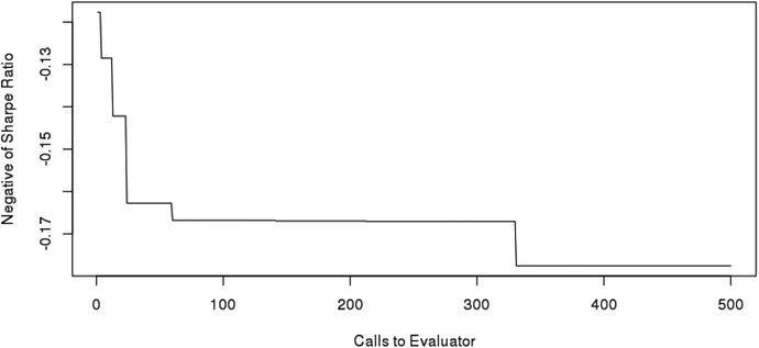
Figure 8-11. Running minimum of objective function for Nelder-Mead
Projecting Trading Performance
Now that we have a sturdy optimization toolbox, we can start using our optimized parameters to simulate real trading performance. The beginning of this chapter discussed the difference between cross validation and curve fitting. If we were to use our optimization algorithms to generate the best parameters for a given time period and then claim we could replicate that performance in production trading, we would be falling victim to curve fitting logic. To project valid and honest results of a strategy, we need to generate optimal parameters in one period and then evaluate them in the following period. The performance of the strategy from the following period is what can be validly and honestly expected in production trading because the means to arriving at such performance figures are replicable in real time. This does not mean we are forced to test purely the optimal parameters in the previous period on the following period. We are allowed to create arbitrarily complex rules for establishing the parameters used in simulation as long as they adhere to the principles of cross validation.
We will define a heuristic using the language of this text for generating valid performance projections.
Define time t where
 , where 1 represents the beginning of the data and T the last time period in the data.
Define D(a,b) as all data and A(a,b) as all account variables such that
 . Define f(θ; D(a, b)) to be the objective function that takes parameter vector θ and data as arguments. Define the optimizer
  such that
![$$ gleft(Dleft(a,b
ight)
ight)=underset{ heta }{argmin}left[fleft( heta; Dleft(a,b
ight)
ight)
ight]. $$](http://images-20200215.ebookreading.net/19/5/5/9781484221785/9781484221785__automated-trading-with__9781484221785__A421454_1_En_8_Chapter_Equh.gif)
Define the simulator
 that returns account variables such that

Define longitudinal step values for optimization and projection as δ O and δ P , respectively, such that 0<δ O ,δ P <T.
Initialize A(0,T) with logical starting values, reflecting holding all cash and no assets for 1,..., T.
For integers i∈[δ O /δ P ],...,[T/δ P ]
Set
![$$ t= minleft[i{delta}_P,T-{delta}_P
ight] $$](http://images-20200215.ebookreading.net/19/5/5/9781484221785/9781484221785__automated-trading-with__9781484221785__A421454_1_En_8_Chapter_IEq68.gif) .
.Calculate
 .
.Calculate
 .
.
Calculate equity curve, return series, performance metrics, and other desired metrics for
 from data contained in A(0,T).
We will use the functions we have built thus far to write a brief listing performing this heuristic . We have discussed many optimizers but have not wrapped them in functions in order to allow users to experiment with their various outputs and results. For this heuristic, we will wrap our generalized pattern in a function that returns only untransformed parameter values. There is information loss in not keeping the optimization variables in the parent R environment, but this is a necessary sacrifice to incorporate it into this heuristic. You are encouraged to modify any of the functions utilized here to output desired auxiliary information in R list objects for later use .
We will not repeat code here for declaration of the optimize() function. You should wrap any of the three optimization algorithms covered in this chapter in a function and pass parameters y,
minVal, and maxValto it. Add the following return line to end of the function call to evaluate ![]() as defined in our heuristic.
as defined in our heuristic.
optimize(y, minVal, maxVal){# Insert Listing 8.2, 8.4, or 8.5# passing y, minval, and maxval# as parameters.# Make sure y, minVal, and maxVal are not# overwritten anywhere inside the function.# They should remain unaltered from their# supplied values.# Finally, return the named vector of# optimal parameters. This return() statement# will work for any listing you include.return(evaluate(OPTIM[which.min(OPTIM$obj),1:np],minVal, maxVal, transformOnly = TRUE))}
Additionally, when wrapping the optimization, it is suggested users lower the maximum iterations value of K to something more manageable.
Listing 8-6 executes the heuristic with δ O =δ P =1year. The equity curve assembled from this process is a valid cross validation for time series that validly and responsibly estimates the performance of your strategy in the future.
This is a key step often ignored in commercial trading platforms. It is usually possible but strenuous to implement this type of cross validation in a commercial platform.
This heuristic is best left to run overnight. It is the final version of many nested functions and loops developed throughout the book. The final output is a list object of the portfolio, cash, and equity curve information for each year. We have added code at the end to consolidate the equity curve information for quick analysis. Otherwise, this is where post-optimization analysis can get arbitrarily complex based on users’ desire to study trade frequency, recession performance, effects of drawdown schedules, and so on .
Note that we started our simulation in 2004 because our parameters can reach as far back as 150*5 days according to the minVal and maxVal in Listing 8-6.
Listing 8-6. Generating Valid Performance Projections with Cross Validation
minVal <- c(n1 = 1, nFact = 1, nSharpe = 1, shThresh = .01)maxVal <- c(n1 = 150, nFact = 5, nSharpe = 200, shThresh = .99)RESULTS <- list()accountParams <- list ()testRange <- 2004:2015# As defined in heuristic with delta_O = delta_P = 1 yearfor( y in testRange ){PARAM <- optimize(y = y, minVal = minVal, maxVal = maxVal)if( y == testRange[1] ){RESULTS[[as.character(y+1)]] <-evaluate(PARAM, y = y + 1, minVal = minVal, maxVal = maxVal,transform = TRUE, returnData = TRUE, verbose = TRUE )} else {# Pass account parameters to next simulation after first yearstrYear <- as.character(y)aLength <- length(RESULTS[[strYear]][["C"]])accountParams[["C"]] <-(RESULTS[[strYear]][["C"]])[aLength]accountParams[["P"]] <- (RESULTS[[strYear]][["P"]])[aLength]accountParams[["p"]] <- (RESULTS[[strYear]][["p"]])[aLength]RESULTS[[as.character(y+1)]] <-evaluate(PARAM, y = y + 1, minVal = minVal, maxVal = maxVal,transform = TRUE, returnData = TRUE, verbose = TRUE,accountParams = accountParams)}}# extract equity curvefor( y in (testRange + 1) ){strYear <- as.character(y)inYear <- substr(index(RESULTS[[strYear]][["P"]]), 1, 4) == strYearequity <- (RESULTS[[strYear]][["equity"]])[inYear]date <- (index(RESULTS[[strYear]][["P"]]))[inYear]if( y == (testRange[1] + 1) ){equitySeries <- zoo(equity, order.by = date)} else {equitySeries <- rbind(equitySeries, zoo(equity, order.by = date))}}
Figure 8-12 shows the equity curve for our cross-validated trading simulation . The strategy suffered going into 2008, perhaps because it was long-only and had no exit criteria. It is likely the Sharpe Ratio is not a robust enough performance metric for generating optimal parameters at t+1 from information in t.

Figure 8-12. Cross-validated equity curve for long-only MACD
Most importantly, this is an accurate representation of how the strategy would have performed if running from 2005 through 2016 in real time. Fitting a successful strategy to all the data at once simply proves existence of a solution. Discovering an optimization process and a strategy framework that work together to generate consistently good results in cross validation is a significant feat of financial engineering .
Conclusion
Optimization can be a daunting field. We have presented large volumes of code in this chapter that will make up the most flexible and research-centered parts of the code base. Before we move to production trading, Chapter 9 will discuss APIs for sending trades to brokerages. Chapter 10 and on will focus on practical considerations for running your platform daily.