Chapter 14: Computing Power and Sample Size
Computing Sample Size for a t Test
Calculating the Sample Size for a Test of Proportions
Computing Sample Size for a One-Way ANOVA Design
Introduction
In my 26 years as a biostatistician at the Rutgers Robert Wood Johnson Medical School in New Jersey, the most frequent question I was asked was "I'm doing an experiment, how many subjects do I need?" Just about any study, especially one for which you are asking for funding or applying for a grant, will require detailed power and sample size calculations.
For those readers a bit rusty on this subject, the power of a study is the probability that the study will result in a statistically significant finding if the drug or treatment that you are studying is different (hopefully better) than either a placebo or an alternate drug or treatment. For many studies conducted at research labs or universities, powers of 80% or 90% are typical. Very large-scale studies may strive for a power of 95%. Small exploratory studies may be satisfied with powers closer to 70%. The bottom line is that it is unethical and wasteful to begin a study with low power. You will have a low probability of demonstrating the superiority of your drug or intervention, and this negative result may dissuade others from investigating the same drug or intervention when it may actually be beneficial.
Depending on the type of study (comparing means or comparing proportions, for example), there is a set of questions that need to be answered before you can determine the number of subjects you will need for a particular study. SAS Studio includes a Power and Sample Size task that performs this analysis for many of the popular study designs.
Computing Sample Size for a t Test
Let's start with a simple study to compare blood pressure in a group of borderline hypertensive subjects. You want to see if a low dose of a beta blocker will reduce blood pressure. Because these subjects are borderline hypertensive and the trial will be relatively short, you decide that it is ethical to use a placebo as your control.
What information do you need to decide how many subjects you need to recruit in order to have a power of 80%? Let's open up the Power and Sample Size tab. It looks like this:
Figure 1: Power and Sample Size Menu

Use the t Tests selection to begin the sample size calculation for comparing two means. Double-clicking t Tests brings up the following:
Figure 2: Select Type of Test and Sample Size or Power

The pull-down list under Type of t test allows you to select from a one-sample test or a two-sample test (either paired or unpaired). Because your study design called for two unpaired groups, select the two-sample option. Next, you can choose to compute power (for a given sample size) or sample size (for a given power). In addition, you can request the total sample size or the sample size per group. It is the latter choice that is shown in Figure 2.
The next section of the Properties tab asks you to decide if the test is one or two-sided. Most studies of this type are two-sided. You can also decide if you want to assume equal variances in the two groups. Figure 3 shows selections for a two-sided test with equal (pooled) variances.
Figure 3: Select Distribution, 1- or 2-Tailed, and Variance Assumption

The calculation for power requires you to either estimate the means of the two groups or the difference between the two means. The screen shot in Figure 4 shows the different ways that you can enter this information.
Figure 4: Select Ways to Specify Means or Differences

For this example, you are choosing to enter the group means you expect. With this selection, the menu system opens boxes for you to enter the expected mean for each group (Figure 5):
Figure 5: Entering Means for Each Group

By clicking the plus sign above the location where you enter your choices for means, you can calculate sample size for different choices of sample means. Figure 6 shows that you want to compute sample sizes for means of 130 versus 120 (a 10-point difference) and 130 versus 125 (a 5-point difference).
Figure 6: Entering Another Pair of Means

Your final two decisions are to estimate the standard deviation and the desired power. As with other choices in this task, you can enter several selections for each. In Figure 7, you see an estimate of 10 for the standard deviation and two powers: .8 and .9. Note that powers are entered as probabilities (values between 0 and 1) and not as percentages.
Figure 7: Enter the Desired Power

Before you run the task, click the Plots tab and make sure that the box Power by sample size plot is checked. You can let the task scale the power axis or you can specify minimum and maximum powers by checking the two boxes under Range of values (Figure 8):
Figure 8: Requesting a Plot of Power by Sample Size

You are ready to run the task. Figure 9 shows the results in table form, and Figure 10 shows the results in graphical form.
Figure 9: Sample Size per Group in Table Form

Notice the large sample sizes necessary to detect a small difference of 5 points. The lowest sample size per group (n per group = 17) is for the largest difference (130 versus 120) and the lowest power (80%).
The graph of sample size by power will contain a line for each combination of means, standard deviations, and powers that you entered. The final decision of sample size is sometimes a compromise between how many subjects you can recruit (and pay for) and how large a difference you would like to be able to detect.
Figure 10: Plot of Power versus Sample Size

Calculating the Sample Size for a Test of Proportions
What information do you need to compute sample sizes for test of proportions? The decisions for this calculation are simpler than the decisions that you made for comparing means. The reason is that once you select a proportion, the standard deviation can be computed.
The information that you need to perform this calculation is listed below:
• Is the test to be conducted as a one-sided or two-sided test? (Usually two-sided)
• What is your alpha level? (Usually ⍺ = .05)
• What is the proportion in the first group (usually a control group)? If unsure, lean toward .5 (maximum variance)
• How large a difference in proportions do you want to be able to detect? (Or the proportion in group two)
• What power do you want? (You often enter several values such as .8, .85, and .9)
You are now ready to run the Test of proportions task. Double-click this selection in the Power and Sample Size menu to bring up the following screen (as before, the Properties screen is shown in pieces):
Figure 11: Select Type of Test and Solve for Power or Sample Size

For the selection "Type of Test," select Two independent proportions. Next, decide if you want to test for power or sample size. In most cases, you will want to know how many subjects you need to obtain a desired power. You have a choice of calculating total sample size or sample size per group. Here, you chose sample size per group.
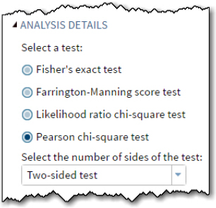
The next part of the Properties screen asks you to select the statistical test that you plan to use in the analysis. For most studies, especially with fairly large n's, the Pearson chi-square test is a good choice. If you believe that you will have small expected values in the study, you may choose Fisher's exact test. Finally, indicate if the test is to be conducted as a one-sided or two-sided test. In Figure 12, you see selections for a Pearson chi-square test conducted as a two-sided test.
Figure 12: Choose the Statistical Method That You Will Be Using
Moving farther down the menu, you see a choice for alpha (the default value of .05 is already entered) and whether you want to enter group proportions or other ways of comparing proportions such as odds ratios or relative risk. The choices in Figure 13 are alpha = .05 and Group proportions. As with the previous calculation where you were comparing means, you can also enter several choices for proportions in the two groups. You decide to compute sample sizes for two different scenarios: one with proportions of .7 and .8, the other with proportions of .7 and .9.
Figure 13: Select Alpha Level and Proportions in the Two Groups

The last entry in the properties tab is to enter one or more values for power. In Figure 14, powers of .8, .85, and .9 were selected.
Figure 14: Select One or More Power Values

Before you run the task, click the Plots tab to request a plot of power by sample size.
Figure 15: Select Plot

It's time to run the task. Click the Run icon to obtain the table and graph displayed in Figure 16 and Figure 17.
Many researchers are shocked when they see the large sample sizes needed to compare proportions. If you look at the N per Group for comparing proportions of .7 and .8 with a power of 90%, you see that you need 392 subjects per group. The smallest number of subjects per group (62) is for proportions of .7 versus .9 with 80% power.
Figure 16: Table of Results

You may find it more instructive to examine the sample size calculations in graphical form. As with the previous situation where you were comparing means, when you compare proportions, you may have to lower your expectations of detecting small differences and design the study with larger differences in the two proportions and, perhaps, slightly lower power.
Figure 17: Graph of Results

Computing Sample Size for a One-Way ANOVA Design
In the current version of SAS Studio, sample size calculations for ANOVA designs are not included in the Power and Sample size task, but they are planned for future releases. If your version of SAS Studio does not include power calculations for ANOVA designs, you can fall back on the "old way" of doing these calculations. That is, run PROC POWER, using the keyword ONEWAYANOVA along with your choices of group means, standard deviations, and power.
The program in Figure 18 computes sample size for a one-way ANOVA design, and you can use this example to help you run PROC POWER for any other one-way design.
In this example, you have made the following decisions:
• There are 3 means estimated to be 20, 25, and 30.
• You have two estimates for standard deviation: 8 and 10
• You want to compute sample size for powers of 80% and 90%.
• You want to compute the n-per-group (as compared to power for a given sample size).
• You would like a plot of Power (x-axis) versus sample size and the axes scaled to show powers from .7 to .9.
Figure 18: Using PROC POWER to Compute Power in an ANOVA Design
title "Computing the Power for an ANOVA Model";
proc power;
onewayanova
groupmeans = 20 | 25 | 30
stddev = 8 10
power = .80 .90
npergroup = .;
plot x = power min = .70 max = .90;
run;
You enter the group means following the key word GROUPMEANS, separating them using a vertical bar (also called a pipe symbol). Follow the keyword STDDEV with one or more estimates of the pooled standard deviation.
You have a choice of computing power or sample size. If you want to compute sample size, enter one or more values for your desired power, and enter a SAS numeric missing value (coded as a period) for the number of subjects per group. If you want to compute power for a given sample size, enter a period for the power and one or more values of sample size.
Use a PLOT statement to indicate that you want power on the x axis, with values of power ranging from .7 to .9. It is time to run the procedure.
The table and graphical output from this procedure are shown in the final two figures:
Figure 19: Table of N per Group for ANOVA Design

Figure 20: Graphical Display of Sample Size Calculations

Conclusions
The SAS Studio statistics tasks include power and sample size calculations for several statistical tests, such as comparing means or comparing proportions. By seeing how to enter data for the two scenarios in this chapter, you should be able to perform calculations for the other designs in the Power and Sample size menu.
Problems
14-1: Compute the sample size per group for the following study:
Two-sample t test.
Two-tailed
Alpha = .05
Mean of group 1: 50
Mean of group 2: 60
Estimated pooled standard deviation: 10
Powers: 80% and 90%
14-2: Compute the sample size per group for the following study:
Two-sample t test.
Two-tailed
Alpha = .05
Mean of group 1: 50
Mean of group 2: 65
Estimated pooled standard deviations: 12 and 15
Powers: 80% and 90%
14-3: Compute the sample size per group for the following study:
ANOVA
Two-tailed
Alpha = .05
Mean of group 1: 50
Mean of group 2: 60
Mean of group 3: 70
Estimated pooled standard deviation: 10
Powers: 80% and 90%
14-4: Compute the sample size per group for the following study:
ANOVA
Two-tailed
Alpha = .05
Mean of group 1: 50
Mean of group 2: 60
Mean of group 3: 65
Estimated pooled standard deviation: 8
Power: 90%
14-5: Compute the sample size per group for the following study:
Test of two proportions
Two-tailed
Alpha = .05
p1 = .7
p2 = .8
Powers: 80% and 90%
14-6: Compute the sample size per group for the following study:
Test of two proportions
Two-tailed
Alpha = .05
p1 = .5
p2 = .75
Power: 80%