Chapter 2
Scalable Data Warehouse Architecture
Abstract
Scalable data warehouses, as a desired solution to some of the problems introduced in the previous chapter, have specific architectural dimensions that are explained in this chapter, including workload, data complexity, query complexity, availability and data latency.
This chapter introduces the architecture of a Data Vault-based data warehouse, including the stage, data warehouse, and information mart layers. In addition, it shows how to use a business vault and other components of the proposed architecture.
Keywords
data complexity
query complexity
data latency
data warehouse
data vault
data architecture
Today’s data warehouse systems make it easy for analysts to access integrated data. In order to achieve this, the data warehouse development team had to process and model the data based on the requirements from the user. The best approach for developing a data warehouse is an iterative development process [1]. That means that the functionality of the data warehouse, as requested by the business users, is designed, developed, implemented and deployed in iterations (sometimes called a sprint or a cycle). In each iteration, more functionality is added to the data warehouse. This is opposite to a “big-bang” approach where all functionality is developed in one large process and finally deployed as a whole.
However, when executing the project, even when using an iterative approach, the effort (and the costs tied to it) to add another functionality usually increases because of existing dependencies that have to be taken care of.
Figure 2.1 shows that the effort to implement the first information mart is relatively low. But when implementing the second information mart, the development team has to maintain the existing solution and take care of existing dependencies, for example to data sources integrated for the first information mart or operational systems consuming information from existing tables. In order to make sure that this previously built functionality doesn’t break when deploying the new functionality for the second information mart, the old functionality has to be retested. In many cases, the existing solution needs to be refactored to maintain the functionality of the individual information marts when new sources are added to the overall solution. All these activities increase the effort for creating the second information mart and, equally, any subsequent information mart or other new functionality. This additional effort is depicted as the rise of the graph in Figure 2.1: once the first information mart is produced, the solution falls into a maintenance mode for all existing functionality. The next project implements another information mart. To implement the second information mart, the effort includes adding the new functionality and maintaining the existing functionality. Because of the dependencies, the existing functionality needs to be refactored and retested regularly.

In other words, the extensibility of many data warehouse architectures, including those presented in Chapter 1, Introduction to Data Warehousing, is not optimal. Furthermore, typical data warehouse architectures often lack dimensions of scalability other than the described dimension of extensibility. We discuss these dimensions in the next section.
2.1. Dimensions of Scalable Data Warehouse Architectures
Business users of data warehouse systems expect to load and prepare more and more data, in terms of variety, volume, and velocity [3]. Also, the workload that is put on typical data warehouse environments is increasing more and more, especially if the initial version of the warehouse has become a success with its first users. Therefore, scalability has multiple dimensions.
2.1.1. Workload
The enterprise data warehouse (EDW) is “by far the largest and most computationally intense business application” in a typical enterprise. EDW systems consist of huge databases, containing historical data on volumes from multiple gigabytes to terabytes of storage [4]. Successful EDW systems face two issues regarding the workload of the system: first, they experience rapidly increasing data volumes and application workloads and, second, an increasing number of concurrent users [5]. In order to meet the performance requirements, EDW systems are implemented on large-scale parallel computers, such as massively parallel processing (MPP) or symmetric multiprocessor (SMP) system environments and clusters and parallel database software. In fact, most medium- to large-size data warehouses could not be implementable without larger-scale parallel hardware and parallel database software to support them [4].
2.1.2. Data Complexity
Another dimension of enterprise data warehouse scalability is data complexity. The following factors contribute to the growth of data complexity [9]:
• Variety of data: nowadays, enterprise organizations capture more than just traditional (e.g., relational or mainframe) master or transactional data. There is an increasing amount of semi-structured data, for example emails, e-forms or HTML and XML files and unstructured data, such as document collections, social network data, images, video and sound files. Another type of data is sensor- and machine-generated data, which might require specific handling. In many cases, enterprises try to derive structured information from unstructured or semi-structured data to increase the business value of the data. While the files may have a structure, the content of the files doesn’t have one. For example, it is not possible to find the face of a specific person in a video without fully processing all frames of the video and building metadata tags to indicate where faces appear in the content.
• Volume of data: the rate at which companies generate and accumulate new data is increasing. Examples include content from Web sites or social networks, document and email collections, weblog data and machine-generated data. The increased data volume leads to much larger data sets, which can run into hundreds of terabytes or even into petabytes of data or beyond.
• Velocity of data: not only the variety and volume of data increases, but the rate at which the data is created also increases rapidly. One example is financial data from financial markets such as the stock exchange. Such data is generated at very high rates and immediately analyzed in order to respond to changes in the market. Other examples include credit card transactions data for fraud detection and sensor data or data from closed-circuit television (CCTV), which is captured for automated video and image analysis in real-time or near-real-time.
• Veracity (trustworthiness) of data: in order to have confidence in data, it must have strong data governance lineage traceability and robust data integration [10].
2.1.3. Analytical Complexity
Due to the availability of large volumes of data with high velocity and variety, businesses demand different and more complex analytical tasks to produce the insight required to solve their business problems. Some of these analyses require that the data be prepared in a fashion not foreseen by the original data warehouse developers. For example, the data that should be fed into a data mining algorithm should have different characteristics regarding the variety, volume and velocity of data.
Consider the example of retail marketing: the campaign accuracy and timeliness need to be improved when moving from retail stores to online channels where more detailed customer insights are required [11]:
• In order to determine customer segmentation and purchase behavior, the business might need historical analysis and reporting of customer demographics and purchase transactions
• Cross-sell opportunities can be identified by analyzing market baskets that show products that can be sold together
• To understand the online behavior of their customers, click-stream analysis is required. This can help to present up-sell offers to the visitors of a Web site
• Given the high amount of social network data and user-generated content, businesses tap into the data by analyzing product reviews, ratings, likes and dislikes, comments, customer service interactions, and so on.
These examples should make it clear that, in order to solve such new and complex analytical tasks, data sources of varying complexity are required. Also, mixing structured and unstructured data becomes more and more common [11].
2.1.4. Query Complexity
When business intelligence (BI) vendors select a relational database management system (RDBMS) for the storage and management of warehouse data, it is a natural choice. Relational databases provide simple data structures and high-level, set-oriented languages that make them ideal for data warehouse applications. The SQL language processors within the database engine map SQL statements into parallel low-level operations to achieve improved query performance (speedup) and enable incremental growth for increased workloads while meeting required levels of performance (scale-up) [12]. Many RDBMSs, such as Microsoft SQL Server, are optimized for data warehouse applications, for example by applying heuristic methods to identify star schema query patterns that are used by the SQL optimizer to improve the query performance of data warehouse applications [13]. Microsoft SQL Server also uses advanced filter techniques to improve query performance by using features such as the bitmap showplan operator [14]. However, some of these features are only available when query statements follow some guidelines (such as using equi-join conditions on INNER joins only) [15].
However, in some cases, queries against the data warehouse can become complex and, given the sheer size of the data warehouse, can take a very long time to complete. Examples include time-series analysis and queries against relational OLAP cubes. For the business analyst, slow response times from the data warehouse are not acceptable because this severely limits productivity [16].
2.1.5. Availability
The data warehouse team is responsible for the availability of the whole data warehouse, including the data marts, reports, OLAP cubes and any other front-end that is used by the business users. In most cases, both parties sign a service level agreement (SLA) that documents the requirements of the business and is the basis for any availability planning of the data warehouse team [17].
The availability of a data warehouse system might be affected by added functionality. One example is the addition of new data sources that have to be loaded and integrated into a new data mart. This, however, would extend the time needed to load all data sources and build the data marts. Parallelization of loads is one solution to the problem because adding more computing resources might ensure the availability of the system. However, the capability to “just add new computing power” must be designed into the data warehouse.
In addition, all major relational database management systems, including the Enterprise edition of Microsoft SQL Server 2014, offer many features, such as partitioning and snapshots, that can help you to meet the availability requirements of the business users. Another option is to create a fail-over cluster to provide an alternative server in the event of an emergency [18].
2.1.6. Security
As data sets grow, the need to secure the data also grows – in fact, the need to secure the data grows exponentially relative to the data set size and variety of data. Security increases the complexity of the system, both in storing the data and in retrieving the data. The larger the data set, the more likely someone can breach the security unnoticed by the rest of the world. The proper and most scalable data warehouses of today and tomorrow will have the right level of security applied from the start of the project. Simply throwing NoSQL at this space doesn’t solve these issues; in fact, it exacerbates them.
The Data Vault 2.0 system of business intelligence aims to assist in solving security, by providing direct integration points in the data model, through the implementation layers, all the way to the architecture and the project components.
2.2. Data Vault 2.0 Architecture
The Data Vault 2.0 architecture addresses the extensibility and dimensions of scalability as defined in the previous section by modifying a typical three-layer data warehouse architecture, which has been introduced in the previous chapter.
As we have outlined in Chapter 1, the primary purpose of an enterprise data warehouse is to provide and present information – that is, aggregated, summarized and consolidated data put into context. To emphasize this ultimate EDW goal, we prefer the term information mart over data mart (which is the term typically used in the BI community).
Other modifications to the typical architecture from Chapter 1 include:
• A staging area which does not store historical information and does not apply any changes to the data, except ensuring the expected data type.
• A data warehouse layer modeled after the Data Vault modeling technique.
• One or more information mart layers that depend on the data warehouse layer.
• An optional Metrics Vault that is used to capture and record runtime information.
• An optional Business Vault that is used to store information where the business rules have been applied. In many cases, the business rules change or alter the data when transforming it into useful information. This is another type of information mart.
• An optional Operational Vault that stores data fed into the data warehouse from operational systems.
• Capabilities for managed self-service BI to allow business users to perform their own data analysis tasks without involvement of IT, including write-back of information into the enterprise data warehouse layer.
All optional Vaults – the Metrics Vault, the Business Vault and the Operational Vault – are part of the Data Vault and are integrated into the data warehouse layer. The reference architecture in the Data Vault 2.0 standard is presented in Figure 2.2.

The Data Vault 2.0 architecture is based on three layers: the staging area, which collects the raw data from the source systems; the enterprise data warehouse layer, modeled as a Data Vault 2.0 model; and the information delivery layer, with information marts as star schemas and other structures. The architecture supports both batch loading of source systems and real-time loading from the enterprise service bus (ESB) or any other service-oriented architecture (SOA). But it is also possible to integrate unstructured NoSQL database systems into this architecture. Due to the platform independence of Data Vault 2.0, NoSQL can be used for every data warehouse layer, including the stage area, the enterprise data warehouse layer, and information delivery. Therefore, the NoSQL database could be used as a staging area and load data into the relational Data Vault layer. However, it could also be integrated both ways with the Data Vault layer via a hashed business key. In this case, it would become a hybrid solution and information marts would consume data from both environments.
However, real-time and NoSQL systems are out of the scope of this book. Therefore, we will concentrate on the relational pieces of the architecture.
One of the biggest differences from typical data warehouse architectures is that most business rules are enforced when building the information marts, and by that are moved towards the end-user. In the Data Vault, there is a distinction between hard and soft business rules. This distinction is discussed in the next section.
2.2.1. Business Rules Definition
In Data Vault 2.0 we distinguish between hard and soft business rules. Generally stated, business rules modify the incoming data to fit the requirements of the business. The distinction between hard and soft business rules is that hard business rules are the technical rules that align the data domains, so-called data type matching. For example, a typical hard business rule is the truncation of source strings that are longer than defined in the stage table. Hard business rules are enforced when the data is extracted from the source systems and loaded into the staging area. These business rules affect only the enforcement of data types (such as string length or Unicode characters) but don’t convert any values to fit the analytical requirements of the business (such as converting between US units and metric units). Other examples of hard business rules include the normalization of hierarchical COBOL copybooks from mainframe systems or XML structures. Also system column computations are examples of hard business rules. As a rule of thumb, hard business rules never change the meaning of the incoming data, only the way the data is stored.
Opposite from hard business rules, soft business rules enforce the business requirements that are stated by the business user. These business rules change the data or the meaning of the data, for example by modifying the grain or interpretation. Examples include the aggregation of data, e.g. allocating the data into categories like income-band, age groups, customer segments, etc., or the consolidation of data from multiple sources. Soft business rules define how the data is aggregated or consolidated. They also define how the data is transformed to meet the requirements of the business.
2.2.2. Business Rules Application
Because we have to align the data types of the source system to those of the staging area tables, we have to enforce hard business rules when loading the staging area (Figure 2.3). This is performed at the latest when inserting the data into the staging area tables because the database management server will check the data types of the inserted data and raise an exception if it is not possible to convert the incoming data to the data type specified in the data definition of the column. This is the case if we try to insert an alphanumeric customer number into an integer-based column, for example, because we expected customer numbers of type “integer.” We can support this process by adding data type conversion logic into the ETL data flow that loads the data into the staging area. By doing so, we’re also implementing hard business rules.

Figure 2.3 Application of hard and soft business rules in a Data Vault enterprise data warehouse.
Hard business rules pose a risk to our ETL routines because if the data violate the rule and this case has not been accounted for, the ETL routine will stop and break the loading process. This is different from soft business rules, which only change the data or the data meaning. Therefore, we need to treat hard business rules differently from soft business rules. We achieve this by separating both rule types from each other.
In typical data warehouse systems, for example the two- and three-layer architectures described in the previous chapter, soft rules are also applied early in the loading process of the data warehouse. This is due to the fact that the data warehouse layer is either a Kimball style star-schema or a normalized data warehouse in third-normal form. In order to fit the data into such structures, the loading ETL data flows have to transform the data to meet the business requirements of the user. This transformation is in effect the implementation of the soft business rules, including required aggregations or consolidation of incoming data. The early implementation of business rules improves the common application of the rules and generally improves the data quality [20].
The problem, however, arises with changes to those business rules. The earlier the business rules are implemented in the architecture of a data warehouse, the more dependencies it has in higher layers of the data warehouse.
Consider the following example from the aviation industry: the aircraft registration number is a standardized alphanumeric identifier for aircraft and is used world-wide. Each number has a prefix that indicates the country where the aircraft is registered. For example, the registration number “D-EBUT” originates from Germany (because of the prefix “D”). Numbers from Germany are actually “smart keys,” a concept that is described in more detail in Chapter 4, Data Vault Modeling. In the case of the German aircraft with the registration “D-EBUT”, the second character indicates that the plane is a single-engine aircraft. In the US, the prefix “N” is common. Until December 31, 1948, there was also a second prefix (the second letter in the number) that was used to indicate the category of the aircraft (see Table 2.1).
Table 2.1
Category Prefixes in the USA until December 1948
| Category | |
| C | Commercial and private airline |
| G | Glider |
| L | Limited |
| R | Restricted (e.g., cropdusters and racing aircrafts) |
| S | State |
| X | Experimental |
For example, the aircraft with the registration number N-X-211 is registered in the experimental category.
However, the FAA decided to stop using the second prefix and now issues numbers between 3 (N1A) and 6 characters (N99999) without any other meaning, except for the first prefix which indicates the origination country. In fact, the second letter is always a number between 1 and 9.
Now, consider the effect of this change on your data warehouse. If the category has been extracted from the (now historic) N-Number, the second letter would be used to identify the aircraft category just after loading the data from the stage area into the normalized data warehouse, where the category would most probably be a column in the aircraft table. Once the numbers change, however, there would be only a number between 1 and 9 in the second position of the registration number, which has no meaning. In order to update the business rule, the easiest approach would be to introduce a new category (“Unknown category”) where those aircraft are mapped to if the second letter in the registration number is from 1 to 9. However, because there will be no new aircraft with a category other than the unknown, it is reasonable to remove the category completely (unless you focus on the analysis of historic aircraft). That makes even more sense if you consider that today’s aircraft are categorized by the operation code, air-worthiness class, and other categories at the same time, making the categorization in Table 2.1 obsolete.
Therefore, this change in the business rule requires the replacement of the category by multiple new categories. In the normalized data warehouse, we would have to remove the old category column and add multiple category references to the aircraft. After changing the ETL jobs that load the data from the stage into the normalized data warehouse, we can change the information mart that is built on top of the data warehouse layer and modify the data mart ETL routines. A couple of questions arise when using this approach:
• How do we deal with historic data in the normalized data warehouse?
• Where do we keep the historic data for later analysis (if required by the business at a later time)?
• How do we analyze both historic aircraft and modern aircraft (a business decision)?
• Will there be multiple dimensions (for the historic category and the modern categories) in the same information mart or multiple information marts for historic and modern aircraft?
• What is the default value for the historic category in modern aircraft?
• What are the default values for the modern categories in ancient aircraft?
In the Data Vault 2.0 architecture, the categorization of an aircraft would be loaded into a table called a satellite that contains descriptive data (we explain the base entities of Data Vault 2.0 modeling in Chapter 4 in detail). When the logic in the source system changes – in this case, the format of the N-Number – the old satellite is closed (no new data is loaded into the current satellite). All new data is loaded into a new satellite with an updated structure that meets the structure of the source data. In this process, there are no business rules implemented. All data is loaded. Because there are now two tables, one holding historic data and the other new data, it is easy to implement the business rule when loading the data from the Data Vault into the information mart. It is also easy to build one information mart for the analysis of historic, older aircraft and another information mart for the analysis of modern aircraft that have been built after 1948.
But the real advantage of separating hard and soft rules becomes clear when thinking about the ETL jobs that need to be adapted to fit the new categorization: none. The ETL jobs that load the historic data remain unchanged and are ready to load more historic data if required (for example, to reload flat files from the archive). The new data is loaded to another target (the second satellite) and is therefore a modified copy of the “historic” ETL routine. Nothing needs to be changed, except the information mart (and its loading routines).
2.2.3. Staging Area Layer
The staging layer is used when loading batch data into the data warehouse. Its primary purpose is to extract the source data as fast as possible from the source system in order to reduce the workload on the operational systems. In addition, the staging area allows the execution of SQL statements against the source data, which might not be the case with direct access to flat files, such as CSV files or Excel sheets.
Note that the staging area does not contain historical data, unlike the traditional architectures described in the previous chapter. Instead only the batch that has to be loaded next into the data warehouse layer is present in the staging area. However, there is an exception to this rule: if there are multiple batches to be loaded, e.g., when an error happened on the weekend and the data from the last couple of days has to be loaded into the data warehouse, there might be multiple batches in the staging area. The primary purpose of having no history in the staging area is not to have to deal with changing data structures. Consider the fact that a source table might change over time. If the staging area kept historic data, there would have to be logic in place for defining the loading procedures into the data warehouse. This logic, in fact business rules, would become more and more complex over time. As we have described in the previous section, the goal of the Data Vault 2.0 architecture is to move complex business rules towards the end-user in order to ensure quick adaption to changes.
The staging area consists of tables that duplicate the structures of the source system. This includes all the tables and columns of the source, including the primary keys. However, indexes and foreign keys, which are used to ensure the referential integrity in the source system, are not duplicated. In addition, all columns are nullable because we want to allow the data warehouse to load the raw data from the source system, including bad data that might exist in the source (especially in flat files). The only business rules that are applied to the incoming data are so-called hard business rules. It is common practice to keep the original names from the source system for naming tables and columns; however, this is not a must.
In addition to the columns from the source system, each table in the stage area includes:
• A sequence number
• A timestamp
• A record source
• Hash key computations for all business keys and their combinations
These fields are metadata information that is required for loading the data into the next layer, the Data Warehouse layer, later on. The sequence number identifies the order of the data in the source system. We can use it when the order within the source is important for loading the data into the data warehouse, e.g., RSS news feeds or transactional data without timestamp information included. The timestamp is the date and time when the record arrives in the data warehouse. The record source indicates the source system from which the data record originates and the hash key is used for identification purposes. A detailed description of these columns is provided in Chapter 4.
2.2.4. Data Warehouse Layer
The second layer in the Data Vault 2.0 architecture is the data warehouse, the purpose of which is to hold all historical, time-variant data. The data warehouse holds raw data, not modified by any business rule other than hard business rules. Therefore, the data is stored in the granularity as provided by the source systems. The data is nonvolatile and every change in the source system is tracked by the Data Vault structure. Data from multiple source systems, but also within a source system, is integrated by the business keys, discussed in Chapter 4. Unlike the information mart, where the information is subject-oriented, the data in the Data Vault is function-oriented.
In batch loading, the data is fed from the staging area, but in real-time loading the data is fed directly from the enterprise service bus (ESB) into the data warehouse. However, as stated before, real-time data warehousing is beyond the scope of this book. We cover the loading of operational data in Chapter 12, which is also applied directly to the data warehouse and follows similar patterns.
2.2.5. Information Mart Layer
Unlike traditional data warehouses, the data warehouse layer of the Data Vault 2.0 architecture is not directly accessed by end-users. Typically, the end-user accesses only the information mart which provides the data in a way that the end-user feels most comfortable with. Because the goal of the enterprise data warehouse is to provide valuable information to its end-users, we use the term information instead of data for this layer. The information in the information mart is subject oriented and can be in aggregated form, flat or wide, prepared for reporting, highly indexed, redundant and quality cleansed. It often follows the star schema and forms the basis for both relational reporting and multidimensional OLAP cubes. Because the end-user accesses only this layer of the data warehouse, having a Data Vault model in the data warehouse layer is transparent to the end-user. If the end-user requires a normalized data warehouse in third-normal form, we can also provide an information mart that meets those needs. Front-end tools are also able to write-back information into the enterprise data warehouse layer.
Other examples for information marts include the Error Mart and the Meta Mart. They are the central location for errors in the data warehouse and the metadata, respectively. Being the central location of this data is also the difference of these two special marts from standard information marts: unlike information marts, the Error and Meta Marts cannot be rebuilt from the Raw Data Vault or any other data source. However, they are similar because end-users, such as administrators, use these marts to analyze errors in the loading process or other problems in the data warehouse, or the metadata that is stored for the data warehouse, its sources and transformations that lead to the information presented in the information marts. Chapter 14, Loading the Dimensional Information Mart, provides an extensive discussion about how to load the information mart for dimensional OLAP cubes from the Data Vault 2.0 structures in the data warehouse.
2.2.6. Metrics Vault
While the three previous layers (the staging area, the data warehouse layer, and the information marts) are mandatory in the Data Vault 2.0 architecture (except for real-time cases which are not covered in this book), the Metrics Vault (covered in this section), the Business Vault (covered in section 2.2.7) and the Operational Vault (covered in section 2.2.8) are optional extensions to the Data Vault 2.0 architecture.
The Metrics Vault is used to capture and record runtime information, including the run history, process metrics, and technical metrics, such as CPU loads, RAM usage, disk I/O metrics and network throughput. Similar to the data warehouse, the Metrics Vault is modeled after the Data Vault 2.0 modeling technique. The data is in its raw format, system or process driven and nonauditable. It might include technical meta-data and technical metrics of the ETL jobs or the data warehouse environment. On top of the Metrics Vault, the Metrics Mart provides the performance metrics information to the user.
Chapter 10, Metadata Management, includes an example of how to track audit information during ETL loads and store the data into a Metrics Vault.
2.2.7. Business Vault
Because some business rules that are applied to the Data Vault 2.0 structures tend to become complex, there is the option to add Business Vault structures to the data warehouse layer. The Business Vault is a sparsely modeled data warehouse based on Data Vault design principles, but houses business-rule changed data. In other words, the data within a Business Vault has already been changed by business rules. In most cases, the Business Vault is an intermediate layer between the Raw Data Vault and the information marts and eases the creation of the end-user structures.
Figure 2.4 shows the Business Vault on top of the Data Vault enterprise data warehouse. This is because the Business Vault is preloaded before the information marts are loaded and eases their loading processes. The complex business rules (the soft rules) source their data from both the Raw Data Vault and the Business Vault entities.
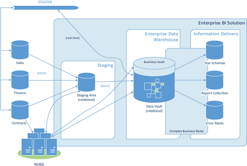
Figure 2.4 Business Vault is located within the Data Vault enterprise data warehouse.
While the Business Vault is modeled after Data Vault 2.0 design principles, it doesn’t have the same requirements regarding the auditability of the source data. Instead, it is possible to drop and regenerate the Business Vault from the Raw Data Vault at any time. The Business Vault provides a consolidated view of the data in the Raw Data Vault to the developers who populate the information marts.
Similar to the Metrics Vault, the Business Vault is not stored in a separate layer. Instead, it is stored as an extension to the Data Vault model within the data warehouse layer. Chapter 14, Loading the Dimensional Information Mart, shows how to use a Business Vault to populate an information mart.
2.2.8. Operational Vault
The Operational Vault is an extension to the Data Vault that is directly accessed by operational systems (Figure 2.5). There are occasions when such systems need to either retrieve data from the enterprise data warehouse or when they need to write data back to it. Examples include master data management (MDM) systems, such as Microsoft Master Data Services (MDS) or metadata management systems. In both cases, there is an advantage of directly operating on the data warehouse layer instead of using an information mart or staging area. Other cases include data mining applications that directly analyze the raw data stored within the data warehouse layer. Often, whenever the interfacing application requires real-time support, whether reading or writing, direct access to the Operational Vault is the best option.

For that reason, integration of real-time data from a service-oriented architecture (SOA) or enterprise service bus (ESB) directly writes into the Operational Vault. While we have defined the Operational Vault as an extension to the Data Vault in the opening of this section, interfacing applications read directly from existing Data Vault structures. Thus, the Data Vault structures become, to some extent, Operational Vault structures.
2.2.9. Managed Self-Service BI
A common experience in data warehousing projects is that, after initial success of the data warehousing initiative, business demands more and more features. However, due to limited team resources in IT, not all requests by the business can be met. In many cases, the requested functionality is only important or applicable to a limited number of business users or has a low business impact. Yet, it is important for those who demand it. But IT has to prioritize their requests in order to use their own IT resources responsibly, with the effect of delayed or completely discarded new features. This low responsiveness to business requests increases discomfort among business users.
An approach called self-service BI allows end-users to completely circumvent IT due to its unresponsiveness. In this approach, business users are left on their own with the whole process of sourcing the data from operational systems, integration, and consolidation of the raw data. There are many problems with this self-service approach that lacks the involvement of IT:
• Direct access to source systems: end-users should not directly access the data from source systems. This exposes raw data that is potentially private and allowing access to this data might circumvent security access, which is implemented in access control lists (ACLs).
• Unintegrated raw data: when sourcing data from multiple source systems, business users are left alone with raw data integration. This can become a tedious and error-prone task if performed manually (e.g., in Microsoft Excel).
• Low data quality: data from source systems often have issues regarding the data quality. Before using the data for analysis, it requires clean up. Again, without the right tools, this can become a burden to the end-user. Or, and that is the worst case, it just doesn’t happen.
• Unconsolidated raw data: in order to analyze the data from multiple source systems, the data often requires consolidation. Without this consolidation, the results from business analysis will be meaningless.
• Nonstandardized business rules: because end-users are dealing with only the raw data in self-service BI, they have to implement all business rules that transform the raw data into meaningful information. But who checks whether this implementation is consistent with the rest of the organization?
In many cases, end-users – even if they are power users with knowledge of SQL, MDX, and other techniques – don’t have the right tools available to solve the tasks. Instead, much work is done manually and is error-prone.
But from our experience, it is not possible to completely prevent such power users from obtaining data from source systems, preparing it, and eventually reporting the data to upper management. What organizations need is a compromise between IT agility and data management that allows power users to obtain the data they need quickly, in a usable quality.
To overcome these problems, the Data Vault 2.0 standard allows experienced or advanced business users to perform their own data analysis tasks on the raw data of the data warehouse. In fact, a Data Vault 2.0 powered IT welcomes business users to take the data that is available in the enterprise data warehouse (either in the Raw Data Vault or in the Business Vault) and use their own tools to transform the data into meaningful information. This is because IT just cannot deliver the requested functionality in the given time frame. Instead, IT sources the raw data from operational systems or other data sources and integrates it using the business key for the Raw Data Vault. IT might also create Business Vault structures to provide a consolidated view on parts of the model or precalculate key performance indicators (KPIs) to ensure consistency among such calculations.
The business user then uses the raw data (from the Raw Data Vault) and the business data (from the Business Vault) to create local information marts using specialized tools. These tools retrieve the data from the enterprise data warehouse, apply a set of user-defined business rules and present the output to the end-user.
This approach is called managed self-service BI and is part of the Data Vault 2.0 standard. In this approach, IT evolves to a service organization that provides those power users with the data they want, in the timeframe they need. The data is integrated by its business key, and, if the end-user wants it, can be consolidated and quality checked. Consolidation and quality checks occur on the way into the Business Vault, as we will show later in this book. The Business Vault also implements some of the most important business rules. The power user has direct access to both the Raw Data Vault and the Business Vault and can, depending on the task at hand, select the raw data or the consolidated, cleaned data. In fact, both types of data are already integrated, so the business user can also join consolidated data with raw data from specific source systems.
This book will demonstrate that loading the raw data into the Raw Data Vault is very easy, including integration using the business keys. In fact, it can be accomplished in short sprint iterations, as we will explain in Chapter 3, Data Vault 2.0 Methodology. When users ask for more data, and this data is not available in the data warehouse, it is possible to source and integrate the data into the Raw Data Vault to provide it to the power user for a managed self-service BI task.
2.2.10. Other Features
The Data Vault 2.0 architecture offers additional capabilities to support real-time (RT) and near-real-time (NRT) environments, unstructured data and NoSQL environments. However, a description of these options is out of the scope of this book.
This chapter introduced the Data Vault 2.0 architecture, a fundamental item in the Data Vault 2.0 standard. The next two chapters will focus on the project methodology and Data Vault modeling, two other fundamental pillars of the Data Vault 2.0 standard.
..................Content has been hidden....................
You can't read the all page of ebook, please click here login for view all page.