Cassandra, by design, can work in a huge cluster across multiple data centers all over the globe. In such a distributed environment, network bandwidth and latency must be critically considered in the architecture, and careful planning in advance is required, otherwise it would lead to catastrophic consequences. The most obvious issue is the time clock synchronization—the genuine means of resolving transaction conflicts that can threaten data integrity in the whole cluster. Cassandra relies on the underlying operating system platform to provide the time clock synchronization service. Furthermore, a node is highly likely to fail at some time and the cluster must be resilient to this typical node failure. These issues have to be thoroughly considered at the architecture level.

Cassandra adopts data replication to tackle these issues, based on the idea of using space in exchange of time. It simply consumes more storage space to make data replicas so as to minimize the complexities in resolving the previously mentioned issues in a cluster.

Data replication is configured by the so-called replication factor in a keyspace. The replication factor refers to the total number of copies of each row across the cluster. So a replication factor of 1 (as seen in the examples in previous chapters) means that there is only one copy of each row on one node. For a replication factor of 2, two copies of each row are on two different nodes. Typically, a replication factor of 3 is sufficient in most production scenarios.

All data replicas are equally important. There are neither master nor slave replicas. So data replication does not have scalability issues. The replication factor can be increased as more nodes are added. However, the replication factor should not be set to exceed the number of nodes in the cluster.

Another unique feature of Cassandra is its awareness of the physical location of nodes in a cluster and their proximity to each other. Cassandra can be configured to know the layout of the data centers and racks by a correct IP address assignment scheme. This setting is known as replication strategy and Cassandra provides two choices for us: SimpleStrategy and NetworkTopologyStrategy.

SimpleStrategy is used on a single machine or on a cluster in a single data center. It places the first replica on a node determined by the partitioner, and then the additional replicas are placed on the next nodes in a clockwise fashion without considering the data center and rack locations. Even though this is the default replication strategy when creating a keyspace, if we ever intend to have more than one data center, we should use NetworkTopologyStrategy instead.

NetworkTopologyStrategy becomes aware of the locations of data centers and racks by understanding the IP addresses of the nodes in the cluster. It places replicas in the same data center by the clockwise mechanism until the first node in another rack is reached. It attempts to place replicas on different racks because the nodes in the same rack often fail at the same time due to power, network issues, air conditioning, and so on.

As mentioned, Cassandra knows the physical location from the IP addresses of the nodes. The mapping of the IP addresses to the data centers and racks is referred to as a snitch. Simply put, a snitch determines which data centers and racks the nodes belong to. It optimizes read operations by providing information about the network topology to Cassandra such that read requests can be routed efficiently. It also affects how replicas can be distributed in consideration of the physical location of data centers and racks.

There are many types of snitches available for different scenarios and each comes with its pros and cons. They are briefly described as follows:

The following figure illustrates an example of a cluster of eight nodes in four racks across two data centers using RackInferringSnitch and a replication factor of three per data center:

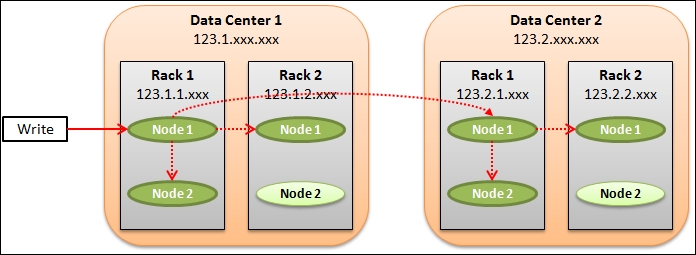
Let us look at the IP address assignment in Data Center 1 first. The IP addresses are grouped and assigned in a top-down fashion. All the nodes in Data Center 1 are in the same 123.1.0.0 subnet. For those nodes in Rack 1, they are in the same 123.1.1.0 subnet. Hence, Node 1 in Rack 1 is assigned an IP address of 123.1.1.1 and Node 2 in Rack 1 is 123.1.1.2. The same rule applies to Rack 2 such that the IP addresses of Node 1 and Node 2 in Rack 2 are 123.1.2.1 and 123.1.2.2, respectively. For Data Center 2, we just change the subnet of the data center to 123.2.0.0 and the racks and nodes in Data Center 2 are then changed similarly.

The RackInferringSnitch deserves a more detailed explanation. It assumes that the network topology is known by properly assigned IP addresses based on the following rule:

IP address = <arbitrary octet>.<data center octet>.<rack octet>.<node octet>

The formula for IP address assignment is shown in the previous paragraph. With this very structured assignment of IP addresses, Cassandra can understand the physical location of all nodes in the cluster.

Another thing that we need to understand is the replication factor of the three replicas that are shown in the previous figure. For a cluster with NetworkToplogyStrategy, the replication factor is set on a per data center basis. So in our example, three replicas are placed in Data Center 1 as illustrated by the dotted arrows in the previous diagram. Data Center 2 is another data center that must have three replicas. Hence, there are six replicas in total across the cluster.

We will not go through every combination of the replication factor, snitch and replication strategy here, but we should now understand the foundation of how Cassandra makes use of them to flexibly deal with different cluster scenarios in real-life production.

Let us return to the Stock Screener Application. The cluster it runs on in Chapter 6, Enhancing a Version, is a single-node cluster. In this section, we will set up a cluster of two nodes that can be used in small-scale production. We will also migrate the existing data in the development database to the new fresh production cluster. It should be noted that for quorum reads/writes, it's usually best practice to use an odd number of nodes.

Global settings

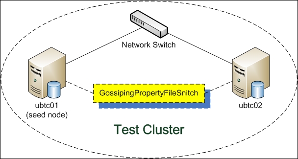
The cluster is named Test Cluster, in which both the ubtc01 and ubtc02 nodes are in the same rack, RACK1, and in the same data center, NY1. The logical architecture of the cluster to be set up is depicted in the following diagram:

In order to configure a Cassandra cluster, we need to modify a few properties in the main configuration file, cassandra.yaml, for Cassandra. Depending on the installation method of Cassandra, cassandra.yaml is located in different directories:

• Package installation: /etc/cassandra/
• Tarball installation: <install_location>/conf/

The first thing to do is to set the properties in cassandra.yaml for each node. As the system configuration of both nodes is the same, the following modification on cassandra.yaml settings is identical to them:

-seeds: ubtc01
listen_address:
rpc_address: 0.0.0.0
endpoint_snitch: GossipingPropertyFileSnitch
auto_bootstrap: false

The reason for using GossipingPropertyFileSnitch is that we want the Cassandra cluster to automatically update all nodes with the gossip protocol when adding a new node.

Apart from cassandra.yaml, we also need to modify the data center and rack properties in cassandra-rackdc.properties in the same location as cassandra.yaml. In our case, the data center is NY1 and the rack is RACK1, as shown in the following code:

dc=NY1
rack=RACK1

Configuration procedure

The configuration procedure of the cluster (refer to the following bash shell scripts: setup_ubtc01.sh and setup_ubtc02.sh) is enumerated as follows:

1. Stop Cassandra service:

   ubtc01:~$ sudo service cassandra stop
   ubtc02:~$ sudo service cassandra stop
   

2. Remove the system keyspace:

   ubtc01:~$ sudo rm -rf /var/lib/cassandra/data/system/*
   ubtc02:~$ sudo rm -rf /var/lib/cassandra/data/system/*
   

3. Modify cassandra.yaml and cassandra-rackdc.properties in both nodes based on the global settings as specified in the previous section
4. Start the seed node ubtc01 first:

   ubtc01:~$ sudo service cassandra start
   

5. Then start ubtc02:

   ubtc02:~$ sudo service cassandra start
   

6. Wait for a minute and check if ubtc01 and ubtc02 are both up and running:

   ubtc01:~$ nodetool status
   

A successful result of setting up the cluster should resemble something similar to the following screenshot, showing that both nodes are up and running:

# -*- coding: utf-8 -*-
# program: chapter07_001.py

# other functions are not shown for brevity

def testcase003():
    ## create Cassandra instance with multiple nodes
    cluster = Cluster(['ubtc01', 'ubtc02'])
    
    ## establish Cassandra connection, using local default
    session = cluster.connect('packtcdma')
    
    start_date = datetime.datetime(2012, 6, 28)
    end_date = datetime.datetime(2013, 9, 28)
    
    ## load the watch list
    stocks_watched = load_watchlist(session, "WS01")
    
    for symbol in stocks_watched:
        ## retrieve data
        data = retrieve_data(session, symbol, start_date, end_date)
        
        ## compute 10-Day SMA
        data = sma(data, 10)
        
        ## generate the buy-and-hold signals
        alerts = signal_close_higher_than_sma10(data)
        
        ## save the alert list
        for index, r in alerts.iterrows():
            insert_alert(session, symbol, index, 
                         Decimal(r['close_price']), 
                         r['stock_name'])
    
    ## close Cassandra connection
    cluster.shutdown()

testcase003()