
Chapter 10
MARGIN ANALYSIS: RISKS
Costs are not like problems, people do not like them to be fixed
In Chapter 9, we compared the respective growth rates of revenues and costs. In this chapter, we will compare all company costs and key profit indicators as a percentage of sales (or production for companies that experience major swings in their inventories of finished goods and work in progress).
The purpose of this analysis is to avoid extrapolating into the future the rate of earnings growth recorded in the past. Just because profits grew by 30% p.a. for two years as a result of a number of factors does not mean they will necessarily keep growing at the same pace going forward.
Earnings and sales may not grow at the same pace owing to the following factors:
- structural changes in production;
- the scissors effect (see Chapter 9);
- simply a cyclical effect accentuated by the company's cost structure. This is what we will be examining in more detail in this chapter.
Section 10.1 HOW OPERATING LEVERAGE WORKS
Operating leverage links variation in activity (measured by sales) with changes in result (either operating profit or net income). Operating leverage depends on the level and nature of the breakeven point.
1/ DEFINITION
Breakeven is the level of activity at which total revenue covers total costs. With business running at this level, earnings are thus zero.
Put another way:
- if the company does not reach breakeven (i.e. insufficient sales), the company posts losses;
- if sales are exactly equal to the breakeven point, profits are zero;
- if the company exceeds its breakeven point, it generates a profit.
2/ CALCULATING THE BREAKEVEN POINT
Before the breakeven point can be calculated, it is vital for costs to be divided up into fixed and variable costs. This classification depends on the period under consideration. For instance, it is legitimate to say that:
- in the long term, all costs are variable, irrespective of their nature. If a company is unable to adjust its cost base, it is not a viable company;
- in the very short term (less than three months), almost all costs are fixed, with the exception of certain direct costs (i.e. certain raw materials);
- from a medium-term perspective, certain costs can be considered variable, e.g. indirect personnel cost.
Before starting to calculate a company's breakeven point, it is wise to define which type of breakeven point is needed. This obvious step is all too commonly forgotten.
For instance, we may want to assess:
- the projected change in the company's earnings in the event of a partial recession with or without a reduction in the company's output;
- the sensitivity of earnings to particularly strong business levels at the end of the year;
- the breakeven point implied by a strategic plan, particularly that resulting from the launch of a new business venture.
The breakeven point can be presented graphically:

The breakeven point is the level of sales at which fixed costs are equal to the contribution margin, which is defined as the difference between sales and variable costs. At the breakeven point, the following equation therefore holds true:
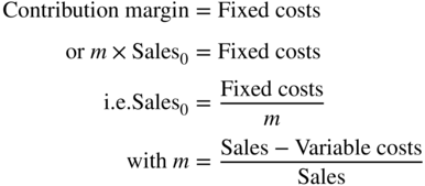
where Sales0 is the level of sales at the breakeven point and m is the contribution margin expressed as a percentage of sales.
In 2021, Exane BNP Paribas estimated that the typical European listed group with a revenue of €100 had €28.5 of fixed costs, €61.1 of variable costs and an operating profit of €10.4. Accordingly, a decrease of 1% in turnover results in a decrease of 3.7% in operating profit. The operating leverage measures the sensitivity of operating result to changes in sales. In this example it is 3.7% / 1% = 3.7.

The above figure rather simplifies things. In fact, fixed costs are not fixed regardless of the level of activity, they are fixed by range of activity and rise or decline in stages.
Some use the term break-even point to measure the moment in the year when a company starts to make profits. Thus, a company with a net income representing 1.1% of its sales will be deemed to start working for its shareholders only from 28 December, i.e. 4 days (1.1% × 365) before the end of the year. This is at most a colourful way of speaking, especially to people with no management skills. In fact, the sales made in the last four days of the year in our example do not constitute full profit because the company still incurs expenses. This is therefore a second abuse of language!
3/ THREE DIFFERENT BREAKEVEN POINTS
The breakeven point may be calculated before or after payments to the company's providers of funds. As a result, three different breakeven points may be calculated:
- operating breakeven, which is a function of the company's fixed and variable production costs that determine the stability of operating profit1;
- financial breakeven, which takes into account the interest costs incurred by the company that determine the stability of profit before tax and non-recurring items;
- total breakeven, which takes into account all the returns required by the company's lenders and shareholders.
Operating breakeven is a dangerous concept because it disregards any return on capital invested in the company, while financial breakeven understates the actual breakeven point because it does not reflect any return on equity, which is the basis of all value creation.
Consequently, we recommend that readers calculate the breakeven point at which the company is able to generate not a zero net income but a positive net income high enough to provide shareholders with the return they require. To this end, we need to adjust the company's cost base by the profit before tax expected by shareholders. Below this breakeven point, the company might generate an accounting profit but will not (totally) satisfy the profitability requirements of its shareholders.
Interest charges represent a fixed cost at a given level of sales (and thus capital requirement). A company that experiences significant volatility in its operating profit may thus compensate partially for this instability through modest financial expense, i.e. by pursuing a strategy of limited debt. In any event, earnings instability is greater for a highly indebted company owing to its financial expense, which represents a fixed cost.
To illustrate these concepts in concrete terms, we have prepared the following table calculating the various breakeven points for ArcelorMittal:2
| 2016 | 2017 | 2018 | 2019 | 2020 | ||
|---|---|---|---|---|---|---|
| Sales | 56,791 | 68,679 | 76,033 | 70,615 | 53,270 | |
| Operating Fixed Costs | FC | 12,495 | 13,979 | 14,474 | 14,418 | 12,606 |
| Financial Fixed Costs | FiC | 1,441 | 427 | 1,558 | 1,207 | 956 |
| Variable Costs | VC | 39,930 | 49,060 | 54,235 | 54,799 | 40,081 |
| Contribution margin as % of sales | 29.7% | 28.6% | 28.7% | 22.4% | 24.8% | |
| Operating breakeven | 42,085 | 48,935 | 50,486 | 64,373 | 50,915 | |
| Position of the company relative to operating breakeven as a % |  | 35% | 40% | 51% | 10% | 5% |
| Financial breakeven | 46,939 | 50,430 | 55,921 | 69,762 | 54,777 | |
| Position of the company relative to financial breakeven |  | 21% | 36% | 36% | 1% | –3% |
| Total breakeven3 | 66,486 | 77,039 | 77,525 | 94,146 | 76,880 | |
| Position of the company relative to total breakeven |  | –15% | –11% | –2% | –25% | –31% |
Based on these considerations, we see that the operating leverage depends on four key parameters:
- the three factors determining the stability of operating profit, i.e. the stability of sales, the structure of production costs and the company's position relative to its breakeven point;
- the level of interest expense, which is itself a function of the debt policy pursued by the company.
From our experience we have seen that, in practice, a company is in an unstable position when its sales are less than 10% above its financial breakeven point. Sales 20% above the financial breakeven point reflect a relatively stable situation and sales more than 20% above the financial breakeven point for a given business structure indicate an exceptional and comfortable situation.
The 2008–2009 and the Covid-19 economic crisis have demonstrated that being 20% above the breakeven point is not enough in cyclical sectors where activity can suddenly collapse by 20%, 30% or 40% as in the cement, steel or car industries.
Section 10.2 A MORE REFINED ANALYSIS PROVIDES GREATER INSIGHT
1/ ANALYSIS OF PAST SITUATIONS
Breakeven analysis (also known as cost–volume–profit analysis) may be used for three different purposes:
- to analyse earnings stability taking into account the characteristics of the market and the structure of production costs;
- to assess a company's real earnings power;
- to analyse the difference between forecasts and actual performance.
(a) Analysis of earnings stability
Here the level of the breakeven point in absolute terms matters much less than the company's position relative to its breakeven point.
When a company is close to its breakeven point, a small change in sales triggers a steep change in its net income, so a strong rate of earnings growth may simply reflect a company's proximity to its breakeven point.
Consider a company with the following manufacturing and sales characteristics:
| Total fixed costs | = | €200,000 |
| Variable costs per unit | = | €50 |
| Unit selling price | = | €100 |
Its breakeven point stands at 4,000 units. To make a profit, the company therefore has to sell at least 4,000 units.
The following table shows a comparison of the relative increases (or reductions) in sales and earnings at five different sales volumes:
| Sales volumes | Net income | Sensitivity | ||||
|---|---|---|---|---|---|---|
| Number of units sold | % Increase compared to previous level (A) | % Decrease compared to previous level | Amount | % Increase compared to previous level (B) | % Decrease compared to previous level | (B)/(A) |
| 4,000 | 20% | 0 | 100% | |||
| 5,000 | 25% | 16.7% | 50,000 | Infinite | 50% | Infinite |
| 6,000 | 20% | 16.7% | 100,000 | 100% | 37.5% | 5 |
| 7,200 | 20% | 16.7% | 160,000 | 60% | 31% | 3 |
| 8,640 | 20% | 232,000 | 45% | 2.25 | ||
This table clearly shows that the closer the breakeven point, the higher the sensitivity of a company's earnings to changes in sales volumes. This phenomenon holds true both above and below the breakeven point.
Consequently, breakeven analysis helps put into perspective a very strong rate of earnings growth during a good year. Rather than getting carried away with one good performance, analysts should attempt to assess the risks of subsequent downturns in reported profits.
For instance, the two spirits groups Pernod Ricard and Remy Cointreau posted similar sales trends but different earnings trends during 2020 because their proximity to breakeven point was very different. Question 8 on page 178 will ask for your comment on this table:
| Sales | Operating income | |
|---|---|---|
| Pernod Ricard | €8,448m (–8.0%) | €2,260m (–12%) |
| Remy Cointreau | €1,025m (–9.0%) | €214m (–22%) |
Likewise, the sensitivity of a company's earnings to changes in sales depends, to a great extent, on its cost structure. The higher a company's fixed costs, the greater the volatility of its earnings,
For example, in 2020, the decrease in earnings of Nestlé was similar to its turnover (–8.3% vs. –8.9% respectively). This seems consistent for an industry where costs are mainly variable.
| Sales | Operating income | |
|---|---|---|
| Nestlé | CHF 84.3bn (–8.9%) | CHF14.9bn (–8.3%) |
| Bureau Veritas | €4.6bn (–9.8%) | €615m (–26.0%) |
| Vinci | €43.2bn (–10.0%) | €2.9bn (–50.1%) |
In contrast, Vinci posted a drop by 50% in operating income for a sales decrease of only 10%; this is because fixed costs are much higher for construction companies. Bureau Veritas's situation, –26% for operating income with a sales decrease of 10%, is sandwiched between the two extremes of packaged food and construction.
In the event of a jump in activity, Vinci's results will increase much faster than Nestlé's, given the importance of fixed costs for the construction company. Vinci therefore has a high level of operating leverage (or operational leverage).
(b) Assessment of normal earnings power
The operating leverage, which accelerates the pace of growth or contraction in a company's earnings triggered by changes in its sales performance, means that the significance of income statement-based margin analysis should be kept in perspective.
The reason for this is that an exceptionally high level of profits may be attributable to exceptionally good conditions that will not last. In such conditions good performance does not necessarily indicate a high level of structural profitability. This held true for a large number of steel companies in 2021.
Consequently, an assessment of a company's earnings power deriving from its structural profitability drivers needs to take into account the operating leverage and cyclical trends, i.e. are we currently in an expansion phase of the cycle?
(c) Variance analysis
Breakeven analysis helps analysts account for differences between the budgeted and actual performance of a company over a given period.
The following table helps illustrate this:
| Value in absolute terms | Structure | ||||||||||
|---|---|---|---|---|---|---|---|---|---|---|---|
| Budget | Actual (A) | Change | % Difference | Theoretical cost structure (B) | Difference (B) − (A) | ||||||
| Sales | 240 | 180 | −60 | −25% | 180 | − | |||||
| Variable costs | 200 | 156 | −44 | −22% | 150 | −6 | |||||
| Contribution margin | 40 | 24 | −16 | −40% | 30 | −6 | |||||
| Margin | 16.7% | 13.3% | 16.7% | ||||||||
| Fixed costs | 20 | 24 | +4 | +20% | 20 | +4 | |||||
| Earnings | 20 | 0 | -20 | −100% | 10 | −10 | |||||
This table shows the collapse in the company's earnings of 20 is attributable to:
- the fall in sales (−25%);
- the surge in fixed costs (+20%);
- the surge in variable costs as a proportion of sales from 83.33% to 86.7%.
The cost structure effect accounts for 50% of the earnings decline (4 in higher fixed costs and 6 in lower contribution margin), with the impact of sales contraction accounting for the remaining 50% of the decline (10 lost in contribution margin: 30 against 40).
2/ STRATEGIC ANALYSIS
(a) Industrial strategy
A large number of companies operating in cyclical sectors made a mistake by raising their breakeven point through heavy investment. In fact, they should have been seeking to achieve the lowest possible operating leverage and, above all, the most flexible possible cost structure to curb the effects of major swings in business levels on their profitability.
For instance, integration has often turned out to be a costly mistake in the construction sector. Only companies that have maintained a lean cost structure through a strategy of outsourcing have been able to survive the successive cycles of boom and bust in the sector.
In highly capital-intensive sectors and those with high fixed costs (pulp, metal tubing, cement, etc.), it is in companies' interests to use equity financing. Such financing does not accentuate the impact of ups and downs in their sales on their bottom line through the leverage effect of debt, but in fact attenuates their impact on earnings.
When a company finds itself in a tight spot, its best financial strategy is to reduce its financial breakeven point by raising fresh equity rather than debt capital, since the latter actually increases its breakeven point, as we have seen. As an example of this policy, ArcelorMittal raised equity in May 2020.
If the outlook for its market points to strong sales growth in the long term, a company may decide to pick up the gauntlet and invest. In doing so, it raises its breakeven point, while retaining substantial room for manoeuvre. It may thus decide to take on additional debt.
As we shall see in Chapter 35, the only real difference in terms of cost between debt and equity financing can be analysed in terms of a company's breakeven point.
(b) Restructuring
When a company falls below its breakeven point, it sinks into the red. It can return to the black only by increasing its sales, lowering its breakeven point or boosting its margins.
Increasing its sales is only a possibility if the company has real strategic clout in its marketplace. Otherwise, it is merely delaying the inevitable: sales will grow at the expense of the company's profitability, thereby creating an illusion of improvement for a while but inevitably precipitating cash problems.
Lowering the breakeven point entails restructuring industrial and commercial operations, e.g. modernisation, reductions in production capacity, cuts in overheads. The danger with this approach is that management may fall into the trap of believing that it is only reducing the company's breakeven point when actually it is shrinking its business. In many cases, a vicious circle sets in, as the measures taken to lower breakeven trigger a major business contraction, compelling the company to lower its breakeven point further, thereby sparking another business contraction, and so on. See Blackberry or Yahoo as examples.
(c) Analysis of cyclical risks
As we stated earlier, there is no such thing as an absolute breakeven point – there are as many breakeven points as there are periods of analysis. But first and foremost, the breakeven point is a dynamic rather than static concept. If sales fall by 5%, the mathematical formulas will suggest that earnings may decline by 20%, 30% or more, depending on the exact circumstances. In fact, experience shows that earnings usually fall much further than breakeven analysis predicts.
A contraction in market volumes is often accompanied by a price war, leading to a decline in the contribution margin. In this situation, fixed costs may increase as customers are slower to pay; inventories build up leading to higher interest costs and higher operating provisions. All these factors may trigger a larger reduction in earnings than that implied by the mathematical formulae of breakeven analysis.
Consequently, breakeven point increases while sales decline, as many recent examples show. Any serious forecasting thus requires modelling based on a thorough analysis of the situation. There are a number of examples of this (Toys “R” Us, JCPenney, etc.).
Businesses such as shipping and sugar production, which require substantial production capacity that takes time to set up, periodically experience production gluts or shortages. As readers are aware, if supply is inflexible, a volume glut (or shortage) of just 5% may be sufficient to trigger far larger price reductions (or hikes) (i.e. 30%, 50% and sometimes even more). Europeans witnessed this in 2018, where sugar production capacity increased following the elimination of quotas.
Here again, an analysis of competition (its strength, patterns and financial structure) is a key factor when assessing the scale of a crisis.
Section 10.3 FROM ANALYSIS TO FORECASTING: THE CONCEPT OF NORMATIVE MARGIN
A great deal of the analysis of financial statements for past periods is carried out for the purpose of preparing financial projections. These forecasts are based on the company's past and the decisions taken by management. This section contains some advice about how best to go about this type of exercise.
All too often, it is not sufficient to merely set up a spreadsheet, click on the main income statement items determining EBITDA (or operating profit if depreciation and amortisation are also to be forecast) and then grow all of these items at a fixed rate. This may be reasonable in itself, but implies unreasonable assumptions when applied systematically. Trees do not grow to the sky!
Instead, readers should:
- gain a full understanding of the company and especially the key drivers impacting margins;
- build growth scenarios, as well as possible reactions by the competition, the environment, international economic conditions, etc.;
- draw up projections and analyse the coherence of the company's economic and strategic policy. For example, is its investment sufficient?
To this end, financial analysts have developed the concept of normalised earnings, i.e. a given company in a given sector should achieve an operating margin of x%.
This type of approach is entirely consistent with financial theory, which states that in each sector profitability should be commensurate with the sector's risks and that, sooner or later, these margins will be achieved, even though adjustments may take considerable time (i.e. five years or even more, in any case much longer than they do in the financial markets).
What factors influence the size of these margins? This question can be answered only in qualitative terms and by performing an analysis of the strategic strengths and weaknesses of a company, which are all related to the concept of barriers to entry:
- the degree of maturity of the business;
- the strength of competition and quality of other market players;
- the importance of commercial factors, such as market share, brands, distribution networks, etc.
- the type of industrial process and incremental productivity gains.
This approach is helpful because it takes into consideration the economic underpinnings of margins. Its drawback lies in the fact that analysts may be tempted to overlook the company's actual margin and concentrate more on idealised future theoretical margins.
We cannot overemphasise the importance of explicitly stating and verifying the significance of all forecasts.
Section 10.4 CASE STUDY: ARCELORMITTAL4
The information4 published by ArcelorMittal does not allow the external analyst to break down costs precisely into fixed and variable costs, despite the breakdown given in the appendix to the accounts of the cost of sales item (which accounts for between 88% and 95% of revenues). We have therefore assumed in the table on page 170 that raw material consumption (about 65% of cost of sales), logistics costs and other costs are variable, which does not seem shocking for a processing company. Other expenses were considered fixed (production personnel, administrative and commercial costs, depreciation).
According to our estimates, ArcelorMittal managed to reduce its fixed costs in parallel with the decrease in its turnover until 2016 (–35% for the former and –33% for the latter), which is an excellent industrial performance. The group was getting dangerously close to its operating breakeven point in 2015 (only 4% above) due to an erosion of its contribution margin that went from 25% to 24% over the period between 2012 and 2015. But in 2016, the group launched a major cost reduction programme over three years. As a result, its contribution margin climbed back to 29/30% in 2016–2018, before falling back to 22% in 2019 and 25% in 2020. It is true that the economic context was initially also more favourable with an increase in steel prices in Europe and the United States, thanks to the implementation of customs barriers against Chinese dumping and the reduction of Chinese exports, before deteriorating again with the Covid-19 crisis.
In 2020 ArcelorMittal remains above its operating breakeven point (+5%). The group is, however, below its financial breakeven point and does not cover the profitability requirement of its shareholders (the group is loss making).
SUMMARY
QUESTIONS
EXERCISES
ANSWERS
BIBLIOGRAPHY
NOTES
- 1 A cash operating breakeven point can be computed for which EBITDA equals zero, as only cash operating expenses are taken into account.
- 2 We analyse the table for ArcelorMittal in Section 10.4 of this chapter. We have assumed that costs of sales and selling and marketing costs are all variable costs and that other operating costs are fixed. This is evidently a rough cut but nevertheless gives a reasonable estimate.
- 3 For ArcelorMittal, we have assumed a cost of equity (see Chapter 19) of 15% in 2016–2017 12% thereafter, and a tax rate between 25% and 28%.
- 4 The breakeven table for ArcelorMittal is on page 170.