Data analysts need to use a variety of tools, methods and techniques from the computing, statistics, machine learning, project management and change management disciplines to do their jobs. This chapter provides an introduction and overview of them.

TOOLS

The data analysis area is crowded with tools, and there is constant innovation in existing tools as well as new tools appearing every year. In this section, tools have been grouped into three main categories, databases, programming tools and visualisation packages, but some tools have functionality in more than one category. Although there are some named examples of popular types of tools in this section, there are many more available.

Databases

Databases are systems that store collections of data, which can then be accessed and manipulated as required. The most common type has, for many decades, been RDBMSs, which store information efficiently and are structured according to the relational model.

Although many alternative types of systems have been developed to deal with data that cannot easily fit into this structure, such as those described in the section in this chapter on NoSQL databases, the relational database remains the most popular type.

Relational databases

Relational databases are built on the principles of the relational model which organises data according to the entities that the data belongs to; each entry is typically represented by a separate table.

To organise business data into entities, the properties and relationships of each entity are recorded. This is called data modelling and will be covered in more detail later in this chapter. More information on data modelling can also be found in the books listed for this chapter in the references at the end of this book.

In a relational system, data about employees, for example, would be stored in an Employee table, where each row represents a separate employee and the columns would represent all the attributes of each employee. The entities will be linked together so that it is possible to connect entities, such as connecting an employee with the department that they are allocated to. This would be done by using a common column in both the Employee and Department tables, such as the employee having the department code as one of its values.

There are numerous large, small, proprietary and free/open-source relational database systems available. Popular examples of relational database systems include IBM Db2, Oracle RDBMS, Microsoft Access, Microsoft SQL Server and MySQL.

NoSQL databases

The previous section described relational database systems that are designed to store structured data and be manipulated with SQL. However, these systems do not deal very well with data that cannot easily be structured according to the relational model. This includes data that is structured according to the object-oriented model: transactional data, social media data and textual data such as books, articles, blogs and social media posts. The last few decades have seen a rise in these types of data, and alternative database systems that are designed to deal with these types of data have been gaining popularity. Collectively they have been referred to as NoSQL.

Graph databases One of the alternatives to relational databases is a graph database where individual data elements are connected together to form a mathematical graph – see Figure 3.1. This type of database is designed with a focus on the connection between the individual elements that are stored. It is very suitable for analysis that deals with social interaction between individuals. It is extensively used in analysis of social media where the primary focus is the connections between people, but it can be used in any area where the relationships between elements are the primary focus.

There is extensive mathematical theory about such graphs, but statistical analysis of them and computational processing are not as well established as they are for relational databases. There is not a widely adopted language for querying and manipulating graphs either and each system therefore uses its own proprietary languages.

Figure 3.1 Simple graph data model

Popular examples of graph database systems include GraphDB and Neo4j.

Object-oriented databases In the object-oriented model, each entity is organised according to its attributes, relationships with other entities and the actions that it can undertake. Object-oriented databases are designed to directly support this data model. Although they have been in use for many decades, they are not yet as effective or as popular as relational database systems. However, they do enable more intuitive storage and retrieval of data that is organised in this way.

These databases might not support SQL, and typically use object-oriented programming languages such as Java, C# and Python to retrieve and manipulate the data that they hold.

Examples of object-oriented databases are ObjectDatabase++, Perst, ObjectDB and db4o.

Programming tools

Although code can be written using only a text editor, such as Microsoft’s Notepad, most programmers will use a programming tool that provides many helpful features. Programming tools are also known as software development environments (SDEs) and usually consist of an integrated development environment (IDE).

This environment typically provides the programmer with a number of features such as a software code editor, debugging functionality, a code interpreter and a compiler.

Examples of popular programming languages for data analysis are Java, Python, R, SPSS, SAS and Matlab. The tools used for SPSS, SAS and Matlab are proprietary, specific to the languages and are usually referred to by the same names.

The Java language is popular for use with Hadoop, which combines advanced data storage and data manipulation and is used to process Big Data. The Hadoop development tools are built specifically for this purpose and normally the IDE of choice.

The Python language is a very popular choice for data analysis and there is a vast number of IDEs that can be used to write code. The Spyder IDE is part of the Anaconda distribution and is developed to work well with a number of packages specifically designed for data analysis. Other IDEs include PyCharm, which also includes features for web development, and Jupyter Notebook, which is designed for cloud computing.

R is also a popular language, particularly when dealing with sophisticated or advanced statistical data analysis. It is supported by the Anaconda distribution mentioned above, but can also be used with the R Studio and a number of other IDEs.

There is more information about the programming languages and methods used for data analysis in the following sections.

Software code editor

This SDE feature helps the programmer to write correct code. It is common for it to contain an autocorrect functionality that will guess the words as the analyst types them, similar to what is done in smartphones and tables for dictionary words. It often also lists the different arguments that the function takes so it can be assured that they are all provided. If there are any potential errors in the code, the editor might highlight or mark the relevant code, similar to spell checkers in text documents.

Debugging functionality

This feature can assist the analyst in finding errors in the code. It will typically allow parts of the code to be executed and the intermediate values of variables and other values to be inspected at that point in the code. The IDE might also have functionality to run the code in a mode that writes detailed information about the execution of the code out to a file.

Interpreter and compiler

The detailed differences between an interpreter and a compiler are not very relevant for data analysts. However, the basic difference is that an interpreter executes the code inside a specific environment, such as the IDE, while a compiler runs it outside an environment.

These features allow the analyst to execute the code and obtain the results of the analysis. The compiler is needed to convert the code into a program that can run on computers that do not have an IDE in the programming language used.

Visualisation packages

Visualisation packages are usually referred to as an interface that can display data in a graphical format, such as graphs, maps, animations and so on. However, analysts should not forget that some types of use still require values for these to be given in a tabular format, such as a spreadsheet. Most of the popular types of visualisation package can also present the data in such tabular formats – often in addition to graphical formats.

Popular visualisation packages include Tableau, Qlikview and the Plotly library.

Interactive aggregations

The packages produced by the vendors mentioned above allow easy interaction by end users. When data analysts have created and calculated data extracts in the appropriate format, these users can often change the filters applied to the data in order to view details on specific regions, products and so on. These packages often have features to allow the end users to choose aggregation levels, to change from a count, a sum, an average and so on.

Graphical displays

The main reason for using visualisation packages is normally to allow end users to see graphical summaries of data analysis. This can be in the form of a chart with various colours showing the numbers. It can also be in the form of geographical maps showing the location of customers, or with regions coloured according to population/customer density. Some advanced packages can produce animations where lines or points on graphs move according to the time of the events.

METHODS

A data analyst needs to be familiar with a wide range of techniques to deal with the different stages of the analysis process and the different types of data that are used. Mastery of all the techniques by individual analysts is rarely possible and data analysis projects are often carried out by teams of specialists. However, effective data analysts will need to have a high level of proficiency in at least one of these skills and strong knowledge of the others.

Data manipulation

The manipulation of data to solve a business problem is the activity that data analysts spend most time doing. It is often said that at least 80 per cent of an analyst’s time is spent on this activity. It is usually the first activity undertaken in a new project, as it is required for any subsequent modelling, statistical analysis, machine learning application or presentation of the information found in the data to the stakeholders concerned.

Although they are often associated with data warehousing, all data manipulation activities can be thought of as a set of three categories of activities known under the acronym ETL: extraction, transformation and loading.

Data can be manipulated with many different programming languages and on a variety of platforms, from large database systems to small local laptops, but the techniques used on all these systems are similar, although the forms might be different.

Data manipulation alone does not reveal any information, but it is essential in transforming the data into a form that is better suited for analysis.

Extraction

Data often has to be taken from a variety of source systems, which keep data in different formats, encodings and internal models. Either a connection will need to be made to these systems to extract the information required, or the systems will need to store the information in a common format.

It is common for relational database systems to provide a connection with the Open Database Connectivity (ODBC) protocol that can serve as a bridge to many other systems and programming languages. For non-relational databases, other protocols exist that can extract information in Extensible Markup Language (XML) or JavaScript Object Notation (JSON) formats, which are a more general-purpose means of encoding data.

Converting data to a common format solves differences such as those that arise when systems from different geographical regions use different ways of representing characters in languages specific to each region; and those that exist when individual operating systems store and encode the data they hold.

Consider this example: an extract from a source system might be required as a snapshot of the relevant data values; or could be required as an initial snapshot, with subsequent extracts of only updated and new values. If the updated and new values have to be integrated with an initial snapshot, further manipulation is likely to be needed in order for the data to be amenable to analysis.

Transformation

Data transformation is the activity of changing the structure of data so that it is easier to analyse. It can cover both cleaning and reformatting of the data, and there is considerable overlap between the two activities. These two activities are often done repeatedly to get the data into a better state for analysis to be done.

Cleaning data Cleaning can improve the overall quality as it relates to data analysis, but if it is over-applied or done badly it can reduce the value of analytical results. If data is not cleaned, analysis could result in inaccurate results, which may lead stakeholders to lose trust in the analysis and also result in poor business decisions and damaged business profits.

There are many ways in which data can be ‘dirty’ and need cleaning:

Reformatting data It is often necessary to use a number of transformations to get data into a format that can be analysed. This problem often stems from the range of different ways data source systems have been designed, with each designed so that it is optimally suited for the purpose it is meant to serve. This can cause difficulties for data analysts trying to analyse data across a broad range of sources.

There can be differences between how the system designers have decided to model the data that their systems hold. An example of this could be a marketing system holding just one record per household, with the occupants identified only as ‘A & B Smith’, whereas the sales system holds two records of ‘Mr Smith’ and ‘Mrs Smith’. In this instance, the data analyst might have difficulties identifying which individual customer reacted to a marketing campaign, and would therefore have to decide to only report which household has reacted rather than which individual.

There can also be differences between how each of the systems records the same information. A system that covers multiple countries may have a free text field for capturing the address, but a system that deals only with one country may have a strict template for entering road, town and postal code in the correct format. Comparing data between the two types can be challenging, and deciding which one to use can affect the accuracy of the analysis.

In data warehousing, the transformation of data is concerned with modelling the data in a form that can be used for presenting it for further analysis. This might involve normalising the data and converting it into a common schema, and might also include building a star or snowflake model (see Figure 3.6) so that users can extract data using an online analytical processing (OLAP) cube tool, which is purpose-built for such tasks.

If the transformation is done merely to enable data to be useful for a specific analytical purpose, some of these activities can be avoided, but the data will still need to be presented in a suitable format, ready for analysis. This often needs to be a tabular format with rows as individual observations and columns as the attributes of each observation.

Loading

Once data has been extracted, cleaned and transformed, it will then need to be transferred to a system where analysis or visualisation of it can be done. Some of the same problems that are faced in the extraction phase can equally apply to the transference. For example, the data will either need to be directly transferred using a common protocol or exported into a text file that can be read by the statistical system in use.

Statistical analysis

Statistical data analysis methods use mathematical techniques to extract insights hidden in data. This involves building mathematical expressions that approximate the data and uses these expressions to generate predictions.

Statistical techniques can be broadly characterised as descriptive or predictive. Each of these statistical themes is a very broad topic and a full exploration is outside the scope of this book; in this section we will merely introduce them as they relate to data analysis.

Bias

Statistical techniques assume that the data to be analysed is a representative sample of all the values that could be generated from the process they are taken from. For the insight and predictions generated from statistical methods to be valid, it is important to ensure that the data is free from any significant bias.

There are many types of bias that originate from the collection and manipulation of data:

Descriptive analytics

Descriptive analytics is also known as summary statistics, and these techniques are used to deduce key information about a data set. They use existing data about past or known events to describe the process that generated the data. They include both simple techniques on just one variable, and more complex techniques on the interactions of several variables.

Examples of simple techniques on a single variable are:

A couple of the more complex descriptive analytics techniques on the interaction between several variables are discussed in the following subsections.

Correlation

The interaction between two variables is described by the correlation between them, and can be expressed by several different statistical measures. If the high values of one variable are often seen together with either high or low values of another variable, then the variables are said to be highly correlated. Although there are many different statistical measures to express the strength of this relationship, the one known as the Pearson coefficient, which is represented by the Greek letter rho (ρ), is the most commonly used and is illustrated in Figure 3.2.¹

Figure 3.2 Examples of correlations in different data sets

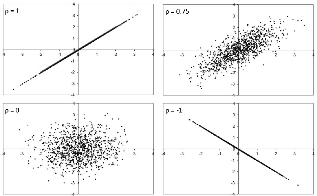
When two variables have a big positive and a big negative number for the Pearson correlation coefficient, between them they are deemed to be highly correlated because the relationship between them is strong.

Significance There are several statistical techniques that can quantify how likely it is to observe a relationship between two variables. It is normally considered significantly interesting and surprising when the observed relationship only has a 1 in 20, or 5 per cent, chance of being randomly generated. This value is normally known as the p-value and the lower this value, the more significant the result is considered.

If repeatedly rolling, say, four fair dice, it will eventually be observed that all four of them lands on a six. Even though it is an unlikely outcome, the large number of experiments (for example, each roll of the dice) will ensure that the outcome is observed and the p-value is large.

With modern computer systems it is possible to analyse many thousands of variables automatically, but when doing so it is almost inevitable that some of them have interesting or surprising relationships. It is important to understand that this might not necessarily be a feature of the variables, but could be merely a feature of the enormous number of automatic tests that the computers are doing.

Predictive analytics

Predictive analytics is used to calculate the expected values of a variable for observations that we have not seen in the data. For example, if we know that one apple costs £1, two apples costs £1.50 and three apples costs £2, then we might propose that apples cost 50p each, plus 50p – and therefore predict that four apples would cost £2.50. Existing or past observations are used to make a generalisation of the process that generates the data, and this is used to predict new values.

Regression An alternative way to represent the relationship between two variables is regression analysis. This technique can be used to describe the relationship between more than two variables where one of the variables is considered dependent on, or predicted by, the other variables. The variable that is predicted is called the dependent variable and the other variables are called independent variables. The mathematics of this model assumes that all the independent variables are uncorrelated, and the correlation technique described earlier in this chapter can be used to verify this condition.

There are a number of models of how the relationship between variables can be represented, and these are known as general linear models. The simplest of these is the linear regression model, where the dependent variable is related to the linear combination of the parameters for the independent variables. The calculation of the regression model is concerned with finding these constant parameters and analysing how well they fit the data.

Often, the data for the dependent and the independent variables needs to be transformed to conform to the requirements for the model and, in this situation, the analyst will need to go back to data manipulation tasks.

When the regression model has been built it can be used to describe what change there would be in the dependent variable given a change in one of the independent variables and assuming all other variables stay the same. This can give the data analyst a good indication of what overall effect each of the independent variables has and the strength of this relationship. It can also be used to predict what values the dependent variable will take in situations that have not been seen in the input data – such as what values it might take in future situations.

Interpolation and extrapolation Many of the statistical models that represent the relationship between different variables, such as the regression models just described, can also be used to predict what values the predicted variable would take when the independent variables take new values. When the model is used to predict new outcomes that are within the range of values for the independent variable it is called interpolation, and when it is used to predict outcomes for input values outside the range of existing values it is called extrapolation (see Figure 3.3).

The distinction between these two types of prediction is important: outcomes that are outside the range of the existing data points are more uncertain, because we have not seen how the process that generates this data behaves in these circumstances.

Figure 3.3 Example of interpolation and extrapolation

Machine learning

Machine learning uses techniques inspired by the way that natural and biological processes react to inputs and adapt to their environment. It involves the building of algorithms capable of making predictions or generalisations directly from input data, without reference to the processes that generate the data.

These techniques can be grouped into two types of algorithms: supervised learning and unsupervised learning.

Supervised learning

In supervised learning, the relationship between input variables and output variables is examined and the outcome can be used to predict likely values for the output, given new values for the input. Many of these techniques do not have the same strict restrictions on the characteristics of the input variables as traditional statistical regression has for its dependent variables. Examples of supervised learning techniques are:

Unsupervised learning

In unsupervised learning, the algorithm is not given an output variable as a target, but only a set of inputs from which it will try to find patterns. The most common type of unsupervised learning is clustering algorithms, which will attempt to group the input observations together in collections that share the same characteristics or are closely related to each other. Of these, the most common and popular type of unsupervised learning algorithms is K-means clustering (Trevino 2016). This has the benefit of being relatively easy to implement on parallel computing platforms and can therefore perform very well on large data sets.

Data visualisation

Visualisation methods make it easier for humans to see patterns in complicated data, and they are also used to communicate the results from traditional statistical or modern machine learning techniques. This approach is focused on how human decision-makers need to have analytical results presented in order to understand them efficiently.

Traditionally, Microsoft Excel has been very extensively used for graphical representations of data, but more advanced data analysis tools, such as R and Python, are becoming common. Both of these languages contain a large range of freely available modules that are able to create very advanced visualisations of data. This includes interactive visualisations in which a programmer develops template web pages which the end user can filter, zoom and rescale to fit their needs. Examples of these modules include matplotlib, seaborn and bokeh for Python and ggplot2 and Plotly for R.

TECHNIQUES

Successful data analysis requires many different techniques. Most of these techniques have been around for decades, but they are being refined for use in our modern Big Data environment. Each technique has strengths and weaknesses, which makes them suitable for specific types of problem.

Programming

Programming languages are used to manipulate data and there are many different variants available; some are designed as general-purpose languages, and some are intended to deal with specific types of problem.

Programming techniques

This section will introduce a number of popular programming techniques and some of the languages in common use in data analysis.

Imperative programming Imperative programming is the most common and widely used technique, both within the data analysis community and in the wider IT development community. This is the technique that most people associate with programming and is often the first style of programming taught in beginner level courses. It owes its popularity to its wide range of powerful applications and its relative ease of use.

In this style of programming, there are three fundamental concepts:

Declarative programming One of the alternatives to imperative programming is the declarative style, where the code will not specify how to achieve the desired outcome, but only what that outcome is.

To delete all the odd numbers from a list, for instance, an imperative program will need to specify the iteration of the list and the selection of the odd numbers, which are then deleted. In the declarative style, the program will merely have to specify the delete operation and the condition for the odd numbers. As can be seen in Figure 3.4, this can lead to very concisely written code.

Figure 3.4 Examples of imperative and declarative code

One very popular example of declarative programming is SQL mentioned earlier. In this language, the actual operations taken to compute the same SELECT statement could be different on systems that are not from the same producer.

Functional programming Using the functional programming approach, the computations never change the data, but create and store new data as a result of manipulations. This approach is inspired by the way mathematical functions operate when there are well-defined input parameters and output data and has its origins in the field of lambda calculus.

Because of its foundations in mathematical theory and extensive research connected to proving the correctness of functions, functional programming is gaining popularity among programmers. This is also because it provides much simpler and easier ways of converting code into parallel execution programs.

Modularisation Procedural languages enable the definition of separate sections of code that achieve specific purposes. A section could be a segment of code used multiple times or used by multiple programs. These individual sections of code are modules that provide specific functionality and they can each build on the functionality of other modules to enable advanced behaviour.

The pre-supplied functions that come with these languages are examples of modules that achieve such specified functionality. They provide well-defined ways to perform simple manipulations of data and are used by programmers to build more complex functionality. Many languages come with a wide library of such modules that have been built by other teams of developers. These teams often make their modules freely available to the community of programmers that use this language. This provides individual programmers with new ways to perform complex data manipulations.

It is also possible for individual programmers and analysts to separate out modules that need to be used multiple times in the same code, or need to be used by multiple pieces of code. These modules could be ones that make a specific calculation used in the organisation or transformation needed for the organisation’s types of information.

When designing and building such modules, it is important to remember the following concepts:

Good software that is well structured and is easy to maintain has a low coupling (relationship between modules) with a high cohesion (relationship within modules). Low coupling often also leads to low cohesion and vice versa, so practical software design is concerned with achieving the best balance between the two.

SQL – the database query language

One of the most popular programming languages for data analysts is SQL. It is a specialist language designed to deal with manipulation of data stored in a RDBMS. It has been an international standard since the late 1980s and has since undergone several reviews and extensions that have expanded the functionality of the language. It is an example of a declarative language.

SQL defines a number of commands that the analyst can use to modify data or change a database in various ways. This includes simple techniques to extract and manipulate data and also advanced optimisation methods and techniques to build applications that use the database to provide other functionalities, such as triggering automatic code to run when certain conditions are met, code that reverses effects when an error has occurred, user defined functions, and many more. Many of these features are not essential for data analysis, however.

A full overview of the extensive abilities of SQL is outside the scope of this book, so this section will merely provide a very short introduction to one part that is essential for data analysts. There are many websites and books which provide more comprehensive coverage of SQL.

SELECT statement The most popular SQL command for data analysts is the SELECT statement, which is used to define a new table with information derived from the existing tables contained in a database. A typical use of this statement is to define a table that is extracted for further processing inside or outside the database.

The SQL SELECT statement consists of a number of clauses that describe what the resulting table should contain. The most important clauses are:

The powerful syntax of the SELECT statement enables analysts to perform a range of advanced data manipulation tasks. The most common tasks are:

In SQL there are also many auxiliary functions that can be used to manipulate individual data values, such as functions to get the absolute value of a number, to get the difference between two dates, to get the upper case of a string and so on.

Advanced query techniques There are many techniques enabling data analysts to write efficient queries that extract data from relational database systems. Comprehensive coverage of these is outside the scope of this book; however, the extraction of information from databases is a crucial skill for data analysts and this section will provide a short introduction to one of the most common techniques.

Query daisy chains: The SELECT statement can be used to extract data from a database for use by other external software, but it can also be used to create new tables that can be stored within the database. This is done by adding a create table clause at the beginning of the statement.

This enables the analyst to use the newly created table in subsequent queries. By using this method sequentially, the analyst can chain the statements together so that each created table is subsequently used to create yet new tables. This technique is essentially daisy chains of queries and can result in complicated code that creates many intermediary tables before arriving at the final table.

An alternative to creating a table is to use the SELECT statement to define a view that is exactly like a table but does not contain any data; this can make subsequent queries perform much faster. This is done be using ‘CREATE VIEW <view_name> AS’ in the above code. A view can be used in any place where a table would be used, and when the database management system sees that a view is used it will calculate its data before continuing with the other code.

Python

The Python language and its associated development environment is becoming very popular among data analysts as it is a powerful language that is free to use and easy to learn. It is an example of a general-purpose language and can be used with a variety of programming styles.

The language consists of a core set of commands which can be extended by downloading packages from a very comprehensive, and free, online repository.² This repository has packages that enable the programmer to do a wide variety of tasks, from working with structured data sets to implementing machine learning algorithms.

Proprietary languages

There exist a number of languages that are used exclusively with particular vendor tools. The best known of these are the languages developed by SPSS, SAS and Matlab. These are suppliers of some of the most popular tools for general data manipulation and statistical calculations. Other popular proprietary languages are described below.

Excel and VBA The syntax used for advanced computations in Microsoft Excel and its companion programming language, VBA, can be used for data manipulation and statistical calculations. Although good for rudimentary data manipulations, they are widely considered to be too limited for more advanced computations where more powerful languages are needed.

Hadoop languages The Apache Hadoop system is a free and open-source system for storing and manipulating massive data sets. It works by combining many smaller computers into a cooperating system where each calculates a small subset of the problem before the results are combined to give the end result.

This system uses a set of specialist programming techniques that are specifically aimed at handling the distributed calculations. It uses the general-purpose Java language to implement the MapReduce programming model, which is a functional programming technique. The Hadoop system also provides limited support for SQL.

Testing

An important part of ensuring that developed code is correct and free from errors is the process of testing the code. Three important types of testing are:

Data modelling and business analysis

Business analysis is the process of identifying the requirements to solve a business need and designing a solution that will satisfy these requirements. The purpose of data modelling is to organise business data into entities and to describe their properties and relationships. Data analysts are often involved in both of these activities, as well as implementing the agreed solution. This is important in order to gain knowledge of the business context of the data and thereby understand the processes that generate that data. It is these processes that the analysis will describe and ultimately change, so it is crucial that data analysts are knowledgeable about them.

Data is a central aspect of most organisations today, and identifying business requirements often involves analysing relevant data about the business problem. This is a central task that involves understanding the business processes, gathering relevant data and extracting information from this data.

Understanding and mapping business processes is a large and complex subject outside the scope of this book. This section will mainly deal with the associated subject of mapping data relationships and data flows.

It is important that data analysts are able to both read and understand such models to be able to effectively extract information from the systems they describe. It is often the case that such models are not available, correct or complete, and so data analysts might need to build data models from scratch.

Relational models

When modelling data in the relational model, data is organised according to the entities that it belongs to. Entities represent anything for which information can be recorded: a physical object, such as a car or person, or an abstract concept such as an organisation or event. The items of information that are recorded for each entity are called attributes and the associations between them are called relations.

Entity-relationship diagrams When modelling data for relational models, it typical to represent these models in entity-relationship diagrams (ER diagrams, see Figure 3.5). These diagrams can be used to develop a model gradually so that it can be implemented in a RDBMS. There are three traditional types of models used:

In a fully developed model, each entry is typically represented by a separate table and its attributes are the columns in the table.

Figure 3.5 Example ER diagram showing a simplified student enrolment system

The data about student entities would be stored in a student table, for instance, where each row represents a student. The columns of the table would represent all the attributes of each student and there would be columns used to link it with entities represented by other tables; for example, a column with an identification code can be used to link to the subjects that the student has enrolled in.

Normalisation One of the advantages of the relational model is that it is capable of storing data in a way that ensures the integrity of the data. Duplication of information in the system, such as when an employee’s salary is recorded in the employee table and the total department salary is recorded in the department table, can lead to errors if the information in one place is updated, inserted or deleted but not in the other.

In relational databases it is very common to use the process of normalisation to eliminate such duplication, which can ensure better organisation, integrity and flexibility of the database. This happens through a process by which the data structures are manipulated into a form where these anomalies are not possible. It is common to talk about data that is structured in unnormalised, 1st, 2nd and 3rd normal form, which gradually reduces the number of anomalies that can occur. Each of these forms is clearly defined and there are even some that define higher forms for specific circumstances.

Data warehouse models

Database systems used to support operational business systems, such as web sales systems, are not very good at supporting analytics. It is important that they are always available and can respond quickly to requests from the users, which usually only involve a small number of records. They are also typically organised in a relational model and normalised to ensure their integrity. In contrast, analytical requests typically involve a large number of records in a batch and, since the data is updated only once a day, the integrity of it becomes less of a concern.

This difference has led to the development of data warehouse systems that read data from the operational systems overnight, when they are not busy, and can be organised to serve the organisation’s analytical needs. The main concern for analytical users is to ensure that data coming from different systems is presented in the same format; for example, in one system a sale might have transaction code 2, while in another it might be transaction code ‘TRN’.

Three-layer architecture It is very common in data warehouses to have a three-layer architecture comprising the following:

Kimball dimensional modelling An alternative to data marts that was developed by Ralph Kimball and called ‘dimensional modelling’ (Kimball and Ross 2013). In this type of model there is one or more fact table, containing one row per object/event being reported, that has a number of defined dimensions.

The customer address could be such a dimension, with a number of levels such as country, town and street. This enables the development of reporting systems known as OLAP cubes to present the total sales by country, and the user can then ‘drill down’ to individual towns, streets or house numbers.

A popular method of logically organising systems that have been modelled in this way is to create a star or snowflake schema, as shown in Figure 3.6.

Object-oriented modelling

In object-oriented modelling, data is organised into a system of interacting objects. It is a model that is used very extensively in software development, and many modern programming languages are organised according to this model. The focus of this approach is the behaviour of each object and particularly how this behaviour is achieved by the collaboration between objects.

Figure 3.6 Example of a star schema

In this model, each object owns its own data, which includes the relationship it holds with other objects. Its behaviour is defined by its public interface, which includes all the commands that it will respond to – also known as functions. Each object can be grouped into collections that will respond to the same commands. For example, a car and a lorry will both be in the group ‘Vehicle’ and therefore respond to the command ‘Drive’ – although they each might do so in different ways.

Unified Modelling Language diagrams Unified Modelling Language (UML) is a modelling language developed to provide a standard for visual representations of the models used in software engineering. The representations are very commonly used for business analysis and object-oriented models. There are 14 diagrams that can be used to represent the structure, behaviour and interactions between objects:

For data analysis, the most important diagrams are the class diagram, which contains the objects with their respective data values, and the use case diagram, which details how users can interact with a system. However, all the diagrams will give important information about a system that is valuable when analysing data.

Change management and project management

Much of the work for data analysts involves projects that change the organisations they are engaged with. Sometimes these projects are done as part of a larger team, and analysts will need to appreciate the contributions of other specialists in the team in order to collaborate effectively with them. Other times, data analysts are not supported by other specialists and will need to undertake some of these responsibilities themselves, such as project management and business change management.

This means that a data analyst needs to be aware of the common project management methods and how they contribute to the success of the change process. There are many project management methods; this section will merely introduce two of the most commonly encountered.

PRINCE2

The PRINCE2 project management method was developed by the UK government in the early 1990s as a way to develop IT projects. It has become a de facto standard for projects in the UK public sector and has been implemented outside the IT industry and gained widespread adoption outside the UK.

The acronym stands for PRojects In a Controlled Environment and the method provides a structured and adaptable framework for managing projects. There is comprehensive guidance for adhering to this framework, which includes qualifications for candidates that pass an accredited exam. The guidance includes seven principles, seven themes and seven processes, as well as 26 suggested management products which are the documentation that can be produced by a project (Bennett and AXELOS 2017).

The seven principles of PRINCE2 are:

The PRINCE2 method has many proponents, but has also attracted some criticism. Although being described by AXELOS, the owners, as suitable for any size of project, it is sometimes considered too formal and comprehensive for smaller organisations or projects. It is also sometimes criticised for not teaching the training course candidates sufficient techniques to use in projects, such as requirements gathering, stakeholder management, financial project appraisals and so on.

Agile

The Agile software development methodology was developed in the early 2000s as an alternative to the prevailing traditional waterfall methods, most notably the PRINCE2 method, that were considered too focused on documentation and following a prescribed process. It was created as a way to ensure that software could be rapidly developed with only the required focus on formality.

The signatories to the Agile Manifesto wanted to develop software that followed four values:

This group of thought leaders also agreed on 12 principles that covered the Agile Alliance. This movement has given rise to a wide variety of techniques and development methods that implement these values and principles.

More information on Agile can be found on the Agile Manifesto website³ and in Measey et al. (2015).

Time-boxing One of the most prevalent features of Agile projects is the adoption of time-boxing for development phases. As opposed to traditional project management methods, where all the features of the final software are documented and agreed before the development is started, in the time-boxing method a limited set of features is agreed to be developed in the next time-box. When a time-box is nearing completion, the features for the next iteration are agreed. This means that fully functional software is rapidly developed, although with limited functionality, and delivered to the customer. With each iteration of a time-box, the customer gets more and more of the functionality until the project completes. In traditional methods, the project’s money or time could run out without a fully functioning system having been developed. The benefit of time-boxing is that even if the requirements for features grow throughout the project, the customer still has functional software.

SUMMARY

This chapter has introduced the variety of tools, methods and techniques that a data analyst needs to use on a fairly regular basis. These come from the areas of computing and statistics, machine learning, programming, and project and change management disciplines. All these areas can fill several books and courses in their own right. It requires in-depth study and continuous improvement of these skills to master them and progress in a career as data analyst. Career development is discussed in Chapter 5.

A specialist set of skills, methods and techniques that has not been covered in this chapter is the best practice and regulatory knowledge needed to handle sensitive data securely and legally. An introduction to this topic is the subject of the next chapter.

1 For more information on the Pearson coefficient, read an introduction here: www.spss-tutorials.com/pearson-correlation-coefficient/

2 See https://pypi.org/project/pip/

3 See http://agilemanifesto.org/