Chapter 2. Framing Data Processing with ML and AI
A mix of applications and data science combined with a broad data corpus delivers powerful capabilities for a business to act on data. With a wide-open field of machine learning (ML) and artificial intelligence (AI), it helps to set the stage with a common taxonomy.
In this chapter, we explore foundational ML and AI concepts that are used throughout this book.
Foundations of ML and AI for Data Warehousing
The world has become enchanted with the resurgence in AI and ML to solve business problems. And all of these processes need places to store and process data.
The ML and AI renaissance is largely credited to a confluence of forces:
-
The availability of new distributed processing techniques to crunch and store data, including Hadoop and Spark, as well as new distributed, relational datastores
-
The proliferation of compute and storage resources, such as Amazon Web Services (AWS), Microsoft Azure, Google Cloud Platform (GCP), and others
-
The awareness and sharing of the latest algorithms, including everything from ML frameworks such as TensorFlow to vectorized queries
AI
For our purpose, we consider AI as a broad endeavor to mimic rational thought. Humans are masters of pattern recognition, possessing the ability to apply historical events with current situational awareness to make rapid, informed decisions. The same outcomes of data-driven decisions combined with live inputs are part of the push in modern AI.
ML
ML follows as an area of AI focused on applying computational techniques to data. Through exposure to sample data, machines can “learn” to recognize patterns that can be used to form predictions. In the early days of computing, data volumes were limited and compute was a precious resource. As such, human intuition weighed more heavily in the field of computer science. We know that this has changed dramatically in recent times.
Deep Learning
Today with a near endless supply of compute resources and data, businesses can go one step further with ML into deep learning (DL). DL uses more data, more compute, more automation, and less intuition in order to calculate potential patterns in data.
With voluminous amounts of text, images, speech, and, of course, structured data, DL can execute complex transformation functions as well as functions in combinations and layers, as illustrated in Figure 2-1.

Figure 2-1. Common nesting of AI, ML, and DL
Practical Definitions of ML and Data Science
Statistics and data analysis are inherent to business in the sense that, outside of selling-water-in-hell situations, businesses that stay in business necessarily employ statistical data analysis. Capital inflow and outflow correlate with business decisions. You create value by analyzing the flows and using the analysis to improve future decisions. This is to say, in the broadest sense of the topic, there is nothing remarkable about businesses deriving value from data.
The Emergence of Professional Data Science
People began adding the term “science” more recently to refer to a broad set of techniques, tools, and practices that attempt to translate mathematical rigor into analytical results with known accuracy. There are several layers involved in the science, from cleaning and shaping data so that it can be analyzed, all the way to visually representing the results of data analysis.
Developing and Deploying Models
The distinction between development and deployment exists in any software that provides a live service. ML often introduces additional differences between the two environments because the tools a data scientist uses to develop a model tend to be fairly different from the tools powering the user-facing production system. For example, a data scientist might try out different techniques and tweak parameters using ML libraries in R or Python, but that might not be the implementation of the tool used in production, as is depicted in Figure 2-2.

Figure 2-2. Simple development and deployment architecture
Along with professional data scientists, “Data Engineer” (or similarly titled positions) has shown up more and more on company websites in the “Now Hiring” section. These individuals work with data scientists to build and deploy production systems. Depending on the size of an organization and the way it defines roles, there might not be a strict division of labor between “data science” and “data engineering.” However, there is a strict division between the development of models and deploying models as a part of live applications. After they’re deployed, ML applications themselves begin to generate data that we can analyze and use to improve the models. This feedback loop between development and deployment dictates how quickly you can iterate while improving ML applications.
Automating Dynamic ML Systems
The logical extension of a tight development–deployment feedback loop is a system that improves itself. We can accomplish this in a variety of ways. One way is with “online” ML models that can update the model as new data becomes available without fully retraining the model. Another way is to automate offline retraining to be triggered by the passage of time or ingest of data, as illustrated in Figure 2-3.

Figure 2-3. ML application with automatic retraining
Supervised ML
In supervised ML, training data is labeled. With every training record, features represent the observed measurements and they are labeled with categories in a classification model or values of an output space in a regression model, as demonstrated in Figure 2-4.

Figure 2-4. Basics of supervised ML
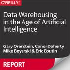
For example, a real estate housing assessment model would take features such as zip code, house size, number of bathrooms, and similar characteristics and then output a prediction on the house value. A regression model might deliver a range or likely range of the potential sale price. A classification model might determine whether the house is likely to sell at a price above or below the averages in its category (see Figure 2-5).
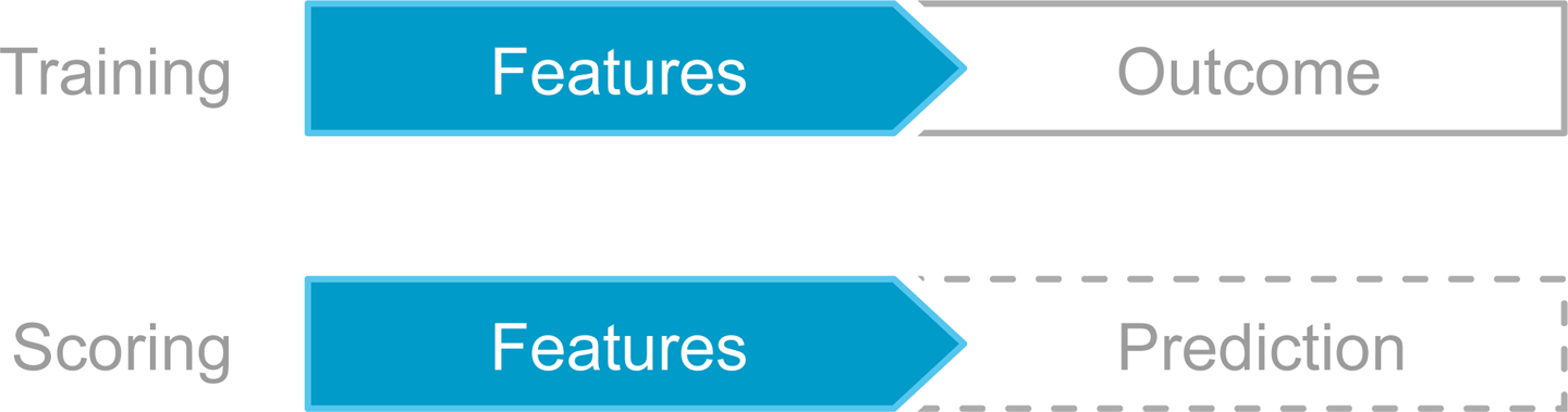
Figure 2-5. Training and scoring phases of supervised learning
A real-time use case might involve Internet of Things (IoT) sensor data from wind turbines. Each turbine would emit an electrical current that can be converted into a digital signal, which then could be analyzed and correlated with specific part failures. For example, one signal might indicate the likelihood of turbine failure, while another might indicate the likelihood of blade failure.
By gathering historical data, training it based on failures observed, and building a model, turbine operators can monitor and respond to sensor data in real time and save millions by avoiding equipment failures.
Regression
Regression models use supervised learning to output results in a continuous prediction space, as compared to classification models which output to a discrete space. The solution to a regression problem is the function that is the most accurate in identifying the relationship between features and outcomes.
In general, regression is a relatively simple way of building a model, and after the regression formula is identified, it consumes a fixed amount of compute power. DL, in contrast, can consume far larger compute resources to identify a pattern and potential outcome.
Classification
Classification models are similar to regression and can use common underlying techniques. The primary difference is that instead of a continuous output space, classification makes a prediction as to which category that record will fall. Binary classification is one example in which instead of predicting a value, the output could simply be “above average” or “below average.”
Binary classifications are common in large part due to their similarity with regression techniques. Figure 2-6 presents an example of linear binary classification. There are also multiclass identifiers across more than two categories. One common example here is handwriting recognition to determine if a character is a letter, a number, or a symbol.

Figure 2-6. Linear binary classifier
Across all supervised learning techniques, one aspect to keep in mind is the consumption of a known amount of compute resources to calculate a result. This is different from the unsupervised techniques, which we describe in the next section.
Unsupervised ML
With unsupervised learning, there are no predefined labels upon which to base a model. So data does not have outcomes, scores, or categories as with supervised ML training data.
The main goal of unsupervised ML is to discern patterns that were not known to exist. For example, one area is the identification of “clusters” that might be easy to compute but are difficult for an individual to recognize unaided (see Figure 2-7).
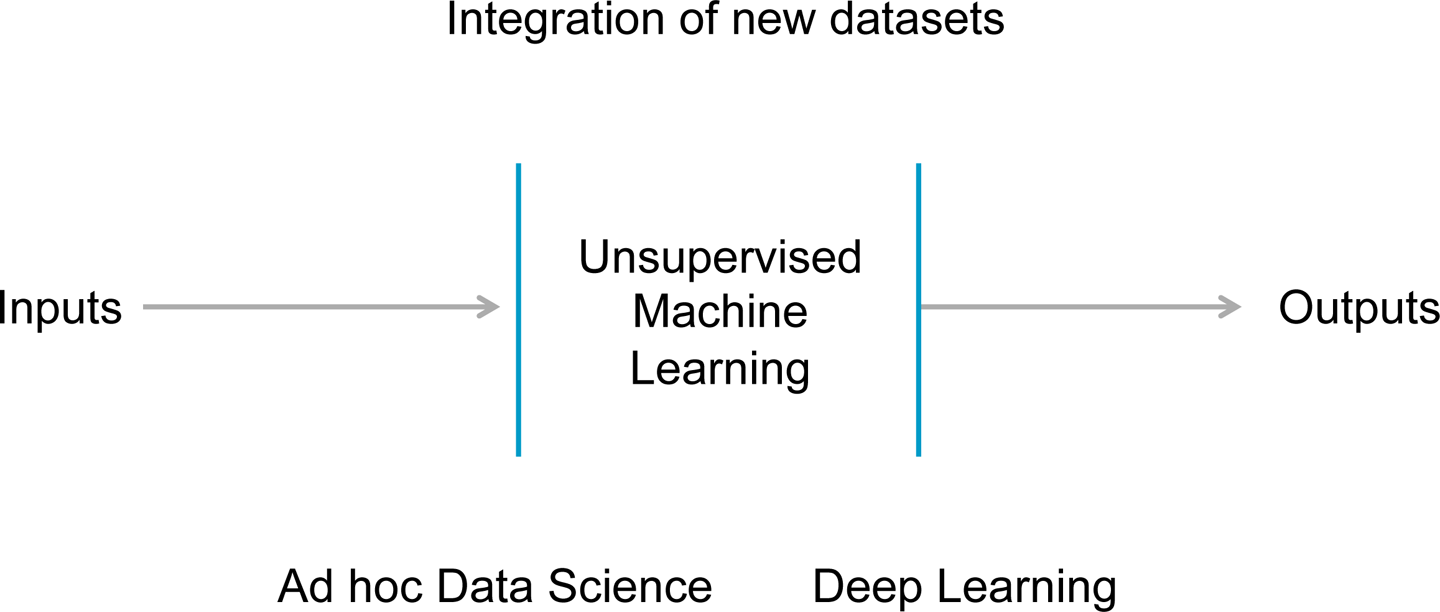
Figure 2-7. Basics of unsupervised ML
The number of clusters that exist and what they represent might be unknown; hence, the need for exploratory techniques to reach conclusions. In the context of business applications, these operations consume an unknown, and potentially uncapped, amount of compute resources putting them more into the data science category compared to operational applications.
Cluster Analysis
Cluster analysis programs detect data patterns when grouping data. In general, they measure closeness or proximity of points within a group. A common approach uses a centroid-based technique to identify clusters, wherein the clusters are defined to minimize distances from a central point, as shown in Figure 2-8.
Figure 2-8. Sample clustering data with centroids determined by k-means
Online Learning
Another useful descriptor for some ML algorithms, a descriptor somewhat orthogonal to the first two, is online learning. An algorithm is “online” if the scoring function (predictor) can be updated as new data becomes available without a “full retrain” that would require passing over all of the original data. An online algorithm can be supervised or unsupervised, but online methods are more common in supervised learning.
Online learning is a particularly efficient way of implementing a real-time feedback loop that adjusts a model on the fly. It takes each new result—for example, “David bought a swimsuit”—and adjusts the model to make other swimsuits a more probable item to show users. Online training takes account of each new data point and adjusts the model accordingly. The results of the updated model are immediately available in the scoring environment. Over time, of course, the question becomes why not align these environments into a single system.
For businesses that operate on rapid cycles and fickle tastes, online learning adapts to changing preferences; for example, seasonal changes in retail apparel. They are quicker to adapt and less costly than out-of-band batch processing.
The Future of AI for Data Processing
For modern workloads, we have passed the monolithic and moved on to the distributed era. Looking beyond, we can see how ML and AI will affect data processing itself. We can explore these trends across database S-curves, as shown in Figure 2-9.

Figure 2-9. Datastore evolution S-curves
The Distributed Era
Distributed architectures use clusters of low-cost servers in concert to achieve scale and economic efficiencies not possible with monolithic systems. In the past 10 years, a range of distributed systems have emerged to power a new S-curve of business progress.
Examples of prominent technologies in the distributed era include, but are certainly not limited to, the following:
-
Message queues like Apache Kafka and Amazon Web Services (AWS) Kinesis
-
Transformation tiers like Apache Spark
-
Orchestration systems like ZooKeeper and Kubernetes
More specifically, in the datastore arena, we have the following:
-
Hadoop-inspired data lakes
-
Key-value stores like Cassandra
-
Relational datastores like MemSQL
Advantages of Distributed Datastores
Distributed datastores provide numerous advantages over monolithic systems, including the following:
- Scale
-
Aggregating servers together enables larger capacities than single node systems.
- Performance
-
The power of many far outpaces the power of one.
- Alignment with CPU trends
-
Although CPUs are gaining more cores, processing power per core has not grown nearly as much. Distributed systems are designed from the beginning to scale out to more CPUs and cores.
Numerous economic efficiencies also come into play with distributed datastores, including these:
- No SANs
-
Distributed systems can store data locally to make use of low-cost server resources.
- No sharding
-
Scaling monolithic systems requires attention to sharding. Distributed systems remove this need.
- Deployment flexibility
-
Well-designed distributed systems will run across bare metal, containers, virtual machines, and the cloud.
- Common core team for numerous configurations
-
With one type of distributed system, IT teams can configure a range of clusters for different capacities and performance requirements.
- Industry standard servers
-
Low-cost hardware or cloud instances provide ample resources for distributed systems. No appliances required.
Together these architectural and economic advantages mark the rationale for jumping the database S-curve.
The Future of AI Augmented Datastores
Beyond distributed datastores, the future includes more AI to streamline data management performance.
AI will appear in many ways, including the following:
- Natural-language queries
-
Examples include sophisticated queries expressed in business terminology using voice recognition.
- Efficient data storage
-
This will be done by identifying more logical patterns, compressing effectively, and creating indexes without requiring a trained database administrator.
- New pattern recognition
-
This will discern new trends in the data without the user having to specify a query.
Of course, AI will likely expand data management performance far beyond these examples, too. In fact, in a 2017 news release, Gartner predicted:
More than 40 percent of data science tasks will be automated by 2020, resulting in increased productivity and broader usage of data and analytics by citizen data scientists.