Chapter 12: Advanced Techniques for Further Speed-Ups

So far, we have discussed all the mainstream distributed Deep Neural Network (DNN) model training and inference methodologies. Here, we want to illustrate some advanced techniques that can be used along with all the previous techniques we have.

In this chapter, we will mainly cover advanced techniques that can be applied generally to DNN training and serving. More specifically, we will discuss general performance debugging approaches, such as kernel event monitoring, job multiplexing, and heterogeneous model training.

Before we discuss anything further, we will list the assumptions we have for this chapter, as follows:

• By default, we will use homogenous GPUs or other accelerators for model training and serving.
• For heterogeneous model training and inference, we will use heterogeneous hardware accelerators for the same training/serving job.
• We have Windows Server so that we can directly use NVIDIA performance debugging tools.
• We will use GPUs or any other hardware accelerators exclusively, which means the hardware is used by a single job only.
• We have high communication bandwidth among all GPUs within a single machine.
• We have low bandwidth for GPU communication across different machines.
• The network between the GPUs is also used by a single training or serving job exclusively.
• If we move the training/serving job among GPUs, we assume the overhead for data movement is just a single shot.
• For model training and serving in a heterogeneous environment, we assume it is easy to achieve load balancing between different accelerators.

First, we will illustrate how to use the performance debugging tools from NVIDIA. Second, we will talk about how to conduct job migration and job multiplexing. Third, we will discuss model training in a heterogeneous environment, which means we use different kinds of hardware accelerators for a single DNN training job.

After going through this chapter, you will understand how to use NVIDIA's Nsight system to conduct performance debugging and analytics. You will also acquire the knowledge of how to do job multiplexing and migration in order to further improve the system efficiency. Last but not least, you will learn how to carry out model training in a heterogeneous environment.

In a nutshell, you will understand the following topics after going through this chapter:

• Debugging and performance analytics
• Job migration and multiplexing
• Model training in a heterogeneous environment

First, we will discuss how to use the performance debugging tools provided by NVIDIA. But before diving into the details, we'll list the technical requirements for this chapter.

Technical requirements

You should be using PyTorch and its relevant platforms for your implementation platform. The main library dependencies for our code are as follows:

• NVIDIA Nsight Graphics >= 2021.5.1
• NVIDIA drivers >=450.119.03
• pip >19.0
• numpy >=1.19.0
• python >=3.7
• ubuntu >=16.04
• cuda >=11.0
• torchvision >=0.10.0

It is mandatory to have the preceding libraries pre-installed with the correct versions.

Debugging and performance analytics

In this section, we will discuss the NVIDIA Nsight performance debugging tool. You will learn how to use this tool for GPU performance debugging.

Before using the tool, you should first download and install it. The web page for downloading is here: https://developer.nvidia.com/nsight-systems.

After downloading and successfully installing the tool, we will learn how to use it. The following is the command line for collecting NVIDIA profiling information using Nsight Systems:

# Profiling

nsys [global-option]

# or

nsys [command-switch][application]

After collecting the profiling information, the system will log all the activities on the GPUs for performance analysis later on.

If your system only has one GPU, you will get the performance information as shown in the following figure:

Figure 12.1 – Single GPU profiling details using the NVIDIA Nsight profiler

As shown in the preceding figure, we can see two devices' logs, one from the CPU and the other from the GPU.

More specifically, the top bars for Thread 3818749824 are all the instructions running on the CPU side. All the bottom bars are CUDA instructions running on Tesla V100-SXM2-16GB, which is on the GPU side.

If your system has more than one GPU, all the device logs will be shown on the same graph. The following figure shows the results of two GPUs plus one CPU profiling:

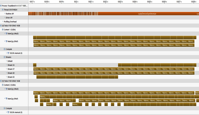
Figure 12.2 – Multi-GPU profiling results from the NVIDIA debugging tool

As shown in the preceding figure, besides the CPU instructions (that is, Thread 3818749824) as the top bars, we have two GPUs' log results.

The first GPU is [4] Tesla V100-SXM2-16GB and the second GPU is [5] Tesla V100-SXM2-16GB.

Here, we conduct some GPU data transfer, which is shown as Memc boxes in Figure 12.2. Memc in Figure 12.2 stands for mem_copy, which basically means copying one GPU's data to another GPU's on-device memory.

So far, we have had a brief overview of what these profiling results look like. Next, we will discuss the general concepts within these profiling results.

General concepts in the profiling results

Since we are focusing on the GPU performance analysis, we will ignore the CPU instruction details here. For the following sections, we will mainly focus on the GPU log results.

Basically, the NVIDIA profiler will log two main things: computation and communication. A simple example of this is as follows:

Figure 12.3 – Simple profiling example including both computation and communication

As shown in the preceding figure, we use GPUs 0, 1, and 2, which are denoted as [0] Tesla P100-SXM2-16GB, [1] Tesla P100-SXM2-16GB, and [4] Tesla P100-SXM2-16GB, separately. They are denoted as such because on the V100 GPU, the yellow bars are too short to be recognized (which means the operations take less time than P100 GPUs).

On the computation side, all the computation events will be shown under the category of Compute in Figure 12.3. Also, each GPU has a single Compute row for monitoring its local computation kernels.

As shown in Figure 12.3, there is no Compute row for GPU 0 (that is, [0] Tesla P100-SXM2-16GB), which means that no computation happens on GPU 0 while this job is running.

For GPU 1 (that is, [1] Tesla-P100-SXM2-16GB), we can see that the compute row exists. It launches four computation kernels, as follows:

• The first is at timestamp 3.869 s.
• The second is between timestamps 3.87 s and 3.871 s.
• The third is at timestamp 3.872 s.
• The fourth is at timestamp 3.873 s.

On the communication side, we can look at the rows under the Context category of each GPU.

For example, on GPU 0 (that is, [0] Tesla-P100-SXM2-16GB) in Figure 12.3, we conducted some MemCpy (PtoP) communication operations from 3.867 s to 3.874 s, which is shown as boxes under Context 1 (CUDA) on GPU 0. Similarly, MemCpy also happens on other GPUs, such as GPU 1 (that is, [1] Tesla-P100-SXM2-16GB) and GPU 4 (that is, [4] Tesla-P100-SXM2-16GB).

Next, we will discuss each category in detail. First, we will discuss the communication analysis among GPUs. Second, we will talk about the computations on each GPU.

Communication results analysis

Here, we discuss the communication patterns in detail. A simple example that covers all the communication patterns is shown in the following figure:

Figure 12.4 – Simple example that covers all communication patterns among GPUs

As shown in the preceding figure, we mainly have three types of data communication among GPUs:

• MemCpy (HtoD): This means we conduct memory copy from Host (H) to Device (D). Host means the CPU and device refers to the current GPU.
• MemCpy (DtoH): This means we conduct memory copy from D to H. It means we transfer data from the GPU to the CPU.
• MemCpy (PtoP): This means we conduct memory copy from Peer to Peer (PtoP). Here, peer means GPU. Thus, PtoP means GPU-to-GPU direct communication without involving the CPU.

Let's take Figure 12.4 as an example. GPU 0 ([0] Tesla V100-SXM2-16GB) has the following communication operations:

1. It first conducts MemCpy (HtoD) (sync), which means it receives data from the CPU side.
2. After that, it conducts MemCpy (PtoP) (async), which means it sends data to another GPU (GPU 1 in this case).
3. After that, it conducts MemCpy (DtoH) (sync), which means it sends data to the CPU side.

Similarly, the data communication pattern also happens on GPU 1.

Next, we will discuss computation results analysis.

Computation results analysis

Here, we will discuss the second main part of performance analysis, that is, computation kernel launching.

Let's first look at an example involving computation that is simpler than Figure 12.3. A simpler version of CUDA/compute kernel launching is as follows:

Figure 12.5 – A GPU job involving two computation kernels on GPU 1 and GPU 4

As shown in the preceding figure, in this simplified version, we have two computation kernels launching on GPU 1 ([1] Tesla-P100-SXM2-16GB) and GPU 4 ([4] Tesla-P100-SXM2-16GB) separately, which are shown in the Compute row.

In addition, by looking at the Streams category, we can see that two compute kernels on each GPU are launched on different streams.

For example, on GPU 1, the first compute kernel is launched on Stream 24, and the second kernel is launched on Stream 25.

Here, each stream on the GPU can be regarded as a thread on the CPU side. The reason for launching multiple streams concurrently is to use the in-parallel computation resource as much as possible.

Now, let's click on the + symbol in front of Compute on GPU 1. We get the following:

Figure 12.6 – Expanding the Compute row to see the kernel information

As shown in the preceding figure, once we expand the Compute category on GPU 1 ([1] Tesla P100-SXM2-16GB), it shows the CUDA/computation kernel name right below the Compute row.

Here, the CUDA kernel we are making a function call to is named pairAddKernel. Basically, it tries to add two large arrays together on the GPU.

If you want to know more details about the kernel information, you can click on each kernel box inside the Compute row. It will show you the detailed kernel information, as shown in the following figure:

Figure 12.7 – CUDA kernel details are shown at the bottom of the table

As shown in the preceding figure, once we click on any computation kernel inside the Compute row, the bottom table shows the details of the computation kernel. Here, it shows the following properties of the computation kernel:

• Compute utilization (4.5%)
• Kernel session (launching time) (12.99123 s)
• Kernel duration (588.02615 ns)

So far, we have discussed how to use the NVIDIA performance profiler to debug and analyze GPU performance on both the communication and computation sides.

For more details, you may refer to NVIDIA's Nsight official user manual page here: https://docs.nvidia.com/nsight-systems/2020.3/profiling/index.html.

Next, we will discuss the topic of job migration and multiplexing.

Job migration and multiplexing

Here, we'll discuss DNN training job migration and multiplexing. We will first discuss the motivation and operations for job migration.

Job migration

The first thing we will discuss here is why we need job migration. A simple example to understand this operation is shown in the following figure:

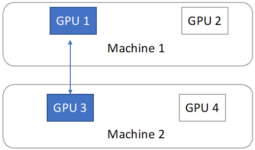
Figure 12.8 – A single training job is assigned to GPU 1 on Machine 1 and GPU 3 on Machine 2

As shown in the preceding figure, in a cloud environment, there is the case that a single DNN training job can be split across multiple machines. As per one of our assumptions at the beginning of this chapter, cross-machine communication bandwidth is low. Therefore, if we conduct frequent model synchronization between GPU 1 and GPU 3, the network communication latency is very high. Thus, the system utilization is very low.

Due to the low system efficiency, we want to move GPUs working on the same job into the minimum number of machines. Merging GPUs into the minimum number of machines is what we call job migration.

In the case of Figure 12.8, we want two GPUs on one machine rather than one GPU on one machine and the other GPU on the other machine. Thus, we conduct job migration by moving all the data and training job operations from GPU 3 to GPU 2, as shown in the following figure:

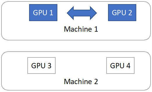
Figure 12.9 – Job migration to Machine 1

As shown in the preceding figure, after the job migration, we move the training job to two GPUs (GPU 1 and GPU 2) located on the same machine (Machine 1). Since the GPU communication bandwidth within one machine is much higher than cross-machine, we improve system efficiency by doing this job migration.

Job multiplexing

Job multiplexing is a general concept to further improve system efficiency. Basically, there are cases where a single job may not fully utilize a GPU's computation power and on-device memory. Thus, we can pack multiple jobs onto the same GPU to improve system efficiency significantly. Packing multiple jobs onto the same GPU is what we called job multiplexing.

A simple example can be when we have two identical training jobs. Each one can utilize 50% of the GPU computation power and 50% of the GPU on-device memory. Thus, instead of training one job at a time, we can pack these two jobs together onto the same GPU and train the two jobs concurrently.

Next, we will discuss how to conduct model training in a heterogeneous environment.

Model training in a heterogeneous environment

This is not a very general case. The motivation for heterogeneous DNN model training is that we may have some legacy hardware accelerators. For example, a company may have used NVIDIA K80 GPUs 10 years ago. Now the company purchases new GPUs such as NVIDIA V100. However, the older K80 GPUs are still usable and the company wants to use all the legacy hardware.

One key challenge of doing heterogeneous DNN model training is load balancing among different hardware.

Let's assume the computation power of each K80 is half of the V100. To achieve good load balancing, if we are doing data parallel training, we should assign N as the mini-batch size on K80 and 2*N as the mini-batch size on V100. If we are doing model-parallel training, we should assign 1/3 layers on K80 and 2/3 layers on V100.

Note that the preceding example for heterogeneous DNN training is simplified. In reality, it is much harder to achieve decent load balancing between different hardware accelerators.

By doing good load balancing between different types of GPUs, we can now conduct a single DNN model training job in a heterogeneous environment.

Summary

In this chapter, we discussed how to conduct performance debugging using NVIDIA profiling tools. We also introduced job migration and job multiplexing schemes to further improve hardware utilization. We also covered the topic of heterogeneous model training using different hardware simultaneously.

After reading this chapter, you should understand how to use NVIDIA Nsight for GPU performance debugging. You should also now know how to conduct job multiplexing and job migration during DNN model training or serving. Finally, you should also have acquired basic knowledge of how to conduct single-job training using different hardware concurrently.

Now, we have completed all the chapters for this book. You should understand the key concepts in distributed machine learning, such as data parallel training and serving, model-parallel training and serving, hybrid data and model parallelism, and several advanced techniques for further speed-ups.