74 6. ROLLOVER CONTROL STRATEGIES AND ALGORITHMS
Without Control
Traditional PID Control
Optimized H∞ Control
0.8
0.6
0.4
0.2
0
-0.2
-0.4
-0.6
-0/8
-1
-1.2
0 2 4 6 8 10
Time (s)
Rollover Index
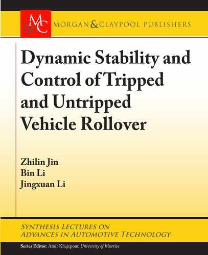
Figure 6.10: Rollover indices of the vehicle under the double-lane change maneuver.
As shown in Figure 6.11, the maximum absolute value of the rollover indices are more than
1 for the vehicle without a controller. So, the vehicle rolls over when it moves in a straight line
or at cornering with an unpredictable bump without control. However, the rollover risk can be
avoided by the differential braking force using a traditional PID control method and optimized
H-infinity control method. Also, it can be found that the maximum value of the rollover index
of vehicle with the optimized H-infinity control method is lower and varies more smoothly
than that with the traditional PID control method in a tripped rollover situation. erefore,
the optimized H-infinity controller can obviously prevent vehicle rollover in a tripped rollover
situation.
6.3 MODEL PREDICTION CONTROL METHOD
Model predictive control features good control effect, strong robustness, and low requirement
for model accuracy and it can be used to control complex process effectively. So, model predictive
control is designed to prevent vehicle rollover by many researchers [35, 64, 65].
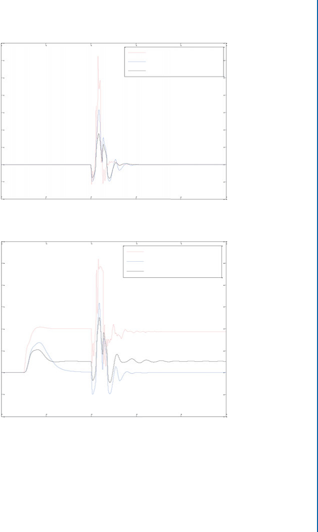
Model prediction control consists of three modules: MPC controller, controlled object,
and state solver. As shown in Figure 6.12, the MPC controller is responsible for combining
the prediction model, objective function and constraint condition to obtain the optimization
solution, getting the optimal control sequence u
.t/ of the current moment, then sending the
6.3. MODEL PREDICTION CONTROL METHOD 75
Without Control
Traditional PID Control
Optimized H∞ Control
1.4
1.2
1
0.8
0.6
0.4
0.2
0
-0.2
-0.4
0 2 4 6 8 10
Time (s)
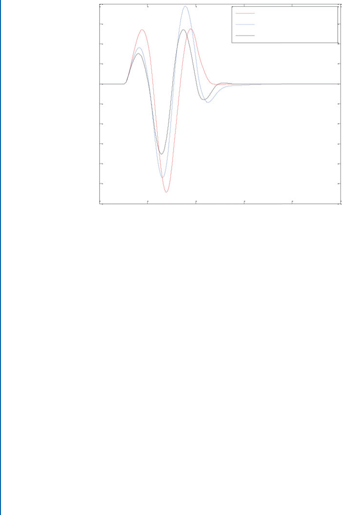
(a) Under a special tripped rollover situation
Rollover Index
Without Control
Traditional PID Control
Optimized H∞ Control
1.2
1
0.8
0.6
0.4
0.2
0
-0.2
-0.4
0 2 4 6 8 10
Time (s)
(b) Under a combined rollover situation
Rollover Index
Figure 6.11: Comparison of the rollover indices under different situations.
76 6. ROLLOVER CONTROL STRATEGIES AND ALGORITHMS
Optimal Solution Prediction Model
Objective Function
Control Constraint
MPC Controller
Controlled Plant
u
*
(t)
y(t)
x(t)
State Solver
xˆ (t)
Figure 6.12: Functional block diagram of Model Predictive Control.
u
.t/ into controlled object. After that, some state values x.t/ of current collection are sent to
state solver. e state solver solves or estimates the state quantity Ox.t / that cannot be obtained
directly from the sensor according to the current state value. After that, Ox.t / is sent into the
MPC controller, make optimal solution again, and the future control sequence is obtained. e
control process of MPC is formed through the calculation of reciprocating.
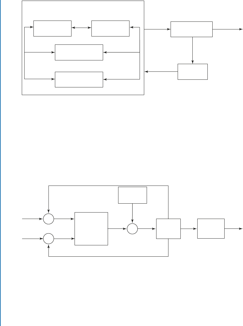
Based on MPC, the strategy of vehicle rollover control is analyzed based on the feedback
of roll angle and yaw rate, as shown in Figure 6.13.
MPC
C
ontroller
Vehicle
M
odel
Conditions
Set
0
δ
u
δ
d
r
Rollover
I
ndex
x(t)
δ
d
φ
Figure 6.13: MPC rollover control strategy based on active steering.
e actual front-wheel steering angle ı is obtained by the accumulation of front-wheel
steering angle ı
0
under setting conditions and control quantity of front-wheel steering angle
ı
u
output by MPC controller. And the controller calculates the control quantity of front-wheel
steering angle ı
u
based on the difference between the actual roll angle and desired roll angle
d
, and the difference between the actual yaw rate r and desired yaw rate r
d
. x.t/ is the vehicle
states which is used to obtain the rollover index. e desired roll angle
d
D 0 and the desired

6.3. MODEL PREDICTION CONTROL METHOD 77
yaw rate can be obtained from the linear 2-DOF model. at is:
r
d
D
uı
L
.
1 C K
e
u
2
/
; (6.19)
where K
e
is the gain of yaw rate.
MPC controller uses following objective function:
J D
P
h
X
j D1
k
y
.
k C j
/
y
d
.
k C j
/
k
2
Q
C
C
h
X
j D1
k
U
.
k C j
/
k
2
R
: (6.20)
In this equation, P
h
is prediction horizon, C
h
is control horizon, Q is the output state
weighting coefficient, R is the control weight coefficient, y represents output state, y
r
represents
output reference value, and U is the control increment.
Moreover,
y
.
k C j
/
D
.
k C j
/
r
.
k C j
/
; y
d
.
k C j
/
D
0
r
d
.
k C j
/
: (6.21)
e vehicle model mentioned in Section 2.3 is used as predictive model and the state-space
equation of predictive model is shown in Equation (6.22):
Px D Ax C Bı
u
; (6.22)
where x is the rollover state quantities of vehicle. A and B are the state space equation matrix.
e model is discretized. According to the first order differential quotient method, the
model can be discretized as discrete state-space equation as follows:
(
x.k C 1/ D A
k
x.k/ C B
k
ı
u
.k/
y.k/ D C
k
x.k/
(6.23)
of which
A
k
D E C t
s
A
B
k
D t
s
B:
(6.24)
In Equations (6.23) and (6.24), E is unit matrix which has the same dimension as A, C
k
is the coefficient matrix in the output equation of state-space equation, t
s
is discrete sampling
time, and t
s
D 0:001.
e objective function needs to calculate the state output of the future time:
.k/ D
"
x.k/
ı
u
.k/
#
: (6.25)
78 6. ROLLOVER CONTROL STRATEGIES AND ALGORITHMS
So, the state-space equation of prediction can be transformed into:
(
.k C 1/ D
O
A
k
.k/ C
O
B
k
ı
u
.k/
y.k/ D
O
C
k
.k/;
(6.26)
where
O
A
k
D
A
k
B
k
0
18
1
;
O
B
k
D
B
k
1
;
O
C
k
D
C
k
0
:
So, the output prediction equation is
Y.k/ D
k
.k/ C ‚
k
ı
u
.k/ (6.27)
of which
Y.k/ D
2
6
6
6
6
6
6
6
4
y.k C 1/
y.k C 2/
: : :
y.k C C
h
/
: : :
y.k C P
h
/
3
7
7
7
7
7
7
7
5
.k/ D
2
6
6
6
6
6
6
6
4
O
C
k
O
A
k
O
C
k
O
A
2
k
: : :
O
C
k
O
A
C
h
k
: : :
O
C
k
O
A
P
h
k
3
7
7
7
7
7
7
7
5
‚.k/ D
2
6
6
6
6
6
6
6
6
6
6
6
6
6
6
4
O
C
k
O
B
k
0 0 0
O
C
k
O
A
k
O
B
k
O
C
k
O
B
k
0 0
: : : : : :
:
:
:
: : :
O
C
k
O
A
C
h
1
k
O
B
k
O
C
k
O
A
C
h
2
k
O
B
k
: : :
O
C
k
O
B
k
O
C
k
O
A
C
h
k
O
B
k
O
C
k
O
A
C
h
1
k
O
B
k
: : :
O
C
k
O
A
k
O
B
k
: : : : : :
:
:
:
: : :
O
C
k
O
A
P
h
1
k
O
B
k
O
C
k
O
A
P
h
2
k
O
B
k
: : :
O
C
k
O
A
P
h
C
h
1
k
O
B
k
3
7
7
7
7
7
7
7
7
7
7
7
7
7
7
5
U.k/ D
2
6
6
6
6
4
ı
u
.k/
ı
u
.k C 1/
: : :
ı
u
.k C C
h
/
3
7
7
7
7
5
:
Because the vehicle model is changing in real time, in order to guarantee the objective
function can obtain the feasible solution at every moment. So, add the relaxation factor to the
optimization goal:
J
.
.k/; ı
u
.k 1/; U.k/
/
D
P
h
X
j D1
k
y.k C j / y
d
.k C j /
k
2
Q
C
C
h
X
j D1
k
U.k C j /
k
2
R
C "
2
1
;
(6.28)
..................Content has been hidden....................
You can't read the all page of ebook, please click here login for view all page.