THE ANNOYANCE: I need to generate a list of names and phone numbers for just those employees who live in Massachusetts—but our employees table includes workers in eight states. I can’t make any sense out of query Design View. Where do I start?

THE FIX: Access’s query Design View really drives people crazy. It’s not intuitive, but once you get used to it it’s really pretty useful. Since querying data is what it’s all about, you must learn how to make query Design View dance to your tune. (Incidentally, Access does have a Simple Query Wizard, which you can find by clicking Insert → Query, but it’s so simple that it’s almost useless.)

To make sense out of the query Design View interface, remember that Access thinks in terms of tables. Tables, and nothing but tables. Even when your query produces a single number, Access thinks of this as a table with one field and one row. So designing a query is really about translating your question into terms that define a new (virtual) table—a.k.a. a recordset. That’s what query Design View helps you do. Here’s how to use it, step by step:

Figure 4-2 shows the finished query in Design View. Switch to Datasheet View, and you can see the query populated with results. Once you understand that all Access ever does is repackage and display data drawn from your underlying tables into new, virtual tables, based on your instructions, you’ll be on your way to Indy 500 query writing—and query Design View will actually start to make sense.

Figure 4-2. This simple query lists the names and phone numbers of employees who live in Massachusetts.

THE ANNOYANCE: We need to generate a list of teachers and the names of the classes each one teaches. We have a teachers table and a classes table, but how do we get them together?

THE FIX: You need to create a multi-table query, and that involves using joins. Joins take a little getting used to, but they are the backbone of complex queries. If you drag multiple tables into the Select query pane without using joins, Access will create one big table with all possible combinations of records. In this example (see Figure 4-3), Access has paired every teacher in tblTeachers with every class in tblClasses, whether a given teacher teaches that class or not. This is known as a “Cartesian” product.

Figure 4-3. All together now! If you drop tables in the query Design View pane and don’t join them, Access will combine them into one big table—not the result you want. Using joins, you can accurately query related data in multiple tables.

Although Cartesian products can sometimes be useful, in this example you really only want rows from tblTeachers (names) to be paired with rows from tblClasses (classes) if the teacher teaches those classes. In other words, you want to match teachers with the classes they teach. That’s where a join comes in—in this case, a join that links the teacherID field in each table.

To create a join in query Design View, go to the upper pane of the Query Design window, then drag the field to join from one table and drop it on the matching field in the other table. The field names do not have to match; the data types must be compatible, but they don’t have to be identical (e.g., you can’t join text to numbers, but you can join Long Integers to Short Integers). Access will create a thin line connecting the two tables (see Figure 4-4). Compare Figure 4-5 with the Cartesian product created earlier, and you can see how the results have been pared down—each teacher only appears with the classes that he or she teaches. You can join on more than one field, but one field often suffices.

Figure 4-4. Tables with joins. Drag-and-drop the join field (here, teacherId) from one table to the other to create a join. This tells Access to include only those rows where the data in the join fields is the same. (The names of the fields do not have to be the same, although in this case they are.)

Figure 4-5. The result of joining tblTeachers and tblClasses on teacherId. Now each teacher appears only with the classes that he or she teaches.

The key to complex queries is understanding that no matter how many tables you add to the upper pane of the Query Design window, Access merges them into a single virtual table. You use joins to tell Access what data you want to cull. Once you’ve specified the joins, you complete your query by adding fields and criteria, exactly as you would in a single-table query. For more on the nuances of joins, see “Data Is Missing from a Multi-Table Query,” later in this chapter.

In a well-designed database, Access may actually create the joins for you automatically. It does this with any fields that are connected by relation-ships; usually, the related fields are the ones that you’d typically want to use for joins. (If, on the other hand, Access automatically creates lots of joins that don’t represent relationships, turn off the AutoJoin function; see “Spurious Joins,” later in this chapter.)

If your data is properly normalized (see “Table Design 101” in Chapter 3), it’s not uncommon for a query to require you to join three or more tables. This can seem daunting at first, but Access can really help. Add one table at a time, create the join you want, and then switch to Datasheet View to make sure you’re getting the data you want. In this way, you can build a complex query in small steps.

THE ANNOYANCE: I created a simple query to extract names and phone numbers from our employees table. I used an expression to concatenate first names and last names, and Access named the column “Expr1.” Can’t the field have a more meaningful name?

THE FIX: When you enter an expression in the Field row of the query design grid, Access generates a generic column name such as “Expr1” or “Expr2” (see Figure 4-6). In queries that run totals, you’ll see names like “CountOfOrderId” and “SumOfTotalAmount.” None of these column headings are very user-friendly. Fortunately, you can change them to any unique name you like. For example, instead of writing your expression as Expr1: [firstName] & " " & [lastName], you could use Full Name: [firstName] & " " & [lastName]. You can also add column names for any fields in the query grid, not just for expressions or aggregate columns—just insert the name, followed by a colon, in the Field line of the query grid. But avoid names that are the same as field names in your tables; this creates ambiguous references that can cause problems. For example, you might be tempted to do something like this: Amount: Nz([Amount]). This is no good. Instead, do something like Amount of Payments: Nz([Amount]).

Figure 4-6. You can replace the generic column name that Access assigns with any unique name you choose.

THE ANNOYANCE: When I created our products table my Access guru told me to leave out the retail price field, since that can be calculated based on other information in the table. Now I need that field in my query, and my guru is on vacation. How can I get it?

THE FIX: Your guru was right. You shouldn’t store data that can be derived from other data by a calculation. The reason comes down to our ever-burning desire to store data in only one place. Experience shows that otherwise your data will eventually get out of sync. In short, you’re doing the right thing—but, of course, you still need that calculated field. Here’s how to create it.

In the Field line of the query design grid, click in a blank column and enter an expression such as RetailPrice: [WholesaleCost] * [MarkupPercent]. (Of course, you’ll use the names of the real fields.) Note that the term before the colon (in this case, “RetailPrice”) can be any unique name you choose. What comes after the colon is the calculation, based on existing fields, functions, constants, and so on. The brackets indicate fields in the table; if you forget to type in the brackets in the Field line, Access will add them for you. When you run the query, Access builds a virtual table with a field named RetailPrice, populated with values based on the expression you wrote. It’s just as if you had a table with that field in it, except that the data in this calculated field will always be up to date.

THE ANNOYANCE: I need a query that computes our average monthly sales figures. I know I have to use a totals query, but I can’t find the command to create it. This is embarrassing.

THE FIX: It is dumb that the Query menu doesn’t have a totals command… but that’s Access for you. The command exists all right, but some brilliant programmer put it on the View menu. In query Design View, click View → Totals, or, if your Query Design toolbar is showing (reveal it by clicking View → Toolbars → Query Design), click the Σ button. Either way, you’ll see a Total line added to the query design grid (with “Group By” in the first cell). Now you’ve got a totals query.

THE ANNOYANCE: I’m trying to find the properties sheet for a query so I can set the Unique Values property to “Yes” and prevent duplicates from coming up. I pressed F4, but nothing happened. I right-clicked the query, but that didn’t display any meaningful properties, either. Where the heck is it?

THE FIX: F4 is such a convenient way of displaying properties sheets that it would have been too sensible for Microsoft to use this technique for opening all properties sheets. As you’ve discovered, it doesn’t work for queries, nor does it work for tables. To display table properties, open the table in Design View (View → Design View) and then click View → Properties. For a query, open it in Design View, right-click in the blank background of the upper pane of the Query Design window, and choose Properties. Note: if you open the properties sheet in SQL View and you click View → Properties, you’ll see some of the properties, but not all of them (see Figure 4-7). Dumb, isn’t it?

Figure 4-7. The properties sheet for the same query, shown in Design View on the left and in SQL View on the right.

THE ANNOYANCE: I need a query that summarizes customer information—specifically, total orders, year-to-date orders, and best month of orders (i.e., the month with the most dollars’ worth of orders). I’m going batty trying to figure out how to combine these into one totals query.

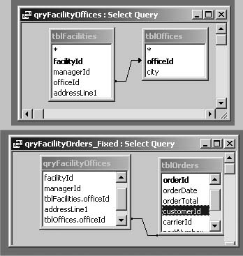
THE FIX: Whenever a query stumps you, the way to start is by looking for one piece of the problem that you know how to solve. In this case, for example, you might already know how to find total orders in a query by itself. That’s going to come in handy, because in query Design View you can use saved queries as building blocks for other queries (see Figure 4-8). This lets you build a complicated solution out of smaller, simpler pieces.

Figure 4-8. This summary query for customer orders is composed of three other queries, joined on customerId. Using simple building blocks can make a complex query easy to create.

While your query may seem dauntingly complex if you think of it as one operation, it becomes simple if you approach it as three separate totals queries (one for total orders, one for year-to-date orders, and one for best month of orders). Once you have these three components, create a blank query and add each of them to it, using the Queries tab of the Show Table dialog. Access treats them just as if they’re tables: you can add any of their fields to the query, and you can join them as appropriate. In a typical case, you’ll want each component query to have a primary key field (such as customerId) that you can join on.

THE ANNOYANCE: I added tables in the upper pane of the Query Design window, and Access created a bunch of spurious join lines. What’s gone wrong, and how can I fix it?

THE FIX: You have AutoJoin enabled, which allows Access to automatically “suggest” joins based on matching field names. Access creates AutoJoins when the data types are compatible, and when one of the fields is a primary key.

To disable AutoJoin, choose Tools → Options, click the Tables/Queries tab, and uncheck the “Enable AutoJoin” box. If relationships are set up properly on your tables, you’ll automatically get joins for those anyway. To remove a spurious join line, simply select it, right-click, and select “Delete.”

THE ANNOYANCE: I wrote a parameter query (see the earlier sidebar “Types of Queries”) so users can pull specific information from our company’s products database on the fly. The only problem? If you make a poor choice of parameters, you can wind up retrieving 250,000 rows—a huge waste of time and network bandwidth. How can I limit the number of records a user gets?

THE FIX: There are two ways, and the one you’ll choose depends on whether you’re querying an Access database directly, or retrieving records from an enterprise database via ODBC or OLEDB. Both settings can be found in the query’s properties sheet. To view the properties sheet, choose View → Design View, right-click in a blank area of the upper pane of the Query Design window, and choose Properties.

If you’re directly querying an Access database, use the Top Values property. Click in the field and choose the value you want from the drop-down list, or type in a custom value (see Figure 4-9). If you use this on a sorted field, you’ll get the first N or N% of the values in sort order; if the field is unsorted, you’ll simply get the first N or N% of the records. For an Access project (a special kind of Access frontend that’s designed for talking to SQL Server) or an ODBC query, use the Max Records property instead. It’s similar to Top Values, but you can specify only absolute numbers, not percentage values.

Figure 4-9. You can select from preset values for the Top Values property, or type in your own value.

THE ANNOYANCE: I created a query that finds all customers who have bought something in the past month, but some customers appear multiple times in the list. Setting Unique Values in the query’s properties sheet doesn’t seem to help. Why not?

THE FIX: When you set the Unique Values field to “Yes,” this tells Access to remove duplicate rows from your results. If Access still gives you duplicate values, it’s usually because you’ve included at least one field in your query that’s different in every record. For instance, if you included a transaction ID in your query, customers with more than one transaction will show up more than once. A row is a true duplicate only if every column is the same as some other row.

Once you find the field that’s different, you have two choices. If you don’t need the field in your query results, uncheck the Show box under that field in the query design grid. If you do need it, make your query a totals query (press the Σ sign on the Query Design toolbar) and group your results by the fields that aren’t changing. For instance, if you want each customer to appear only once in the results, set the Total line to “Group By” for customerId and customer name. But since every field in a totals query must have something on its Total line, you’ll have to choose some aggregate function other than Group By (perhaps First or Last) for the fields that do change.

THE ANNOYANCE: I just inherited a mailing list database with over 30,000 records, and it has lots of duplicate entries. I’m trying to create a query to find the duplicates, but nothing works.

THE FIX: Queries that find duplicates are tricky to write. Even the pros are glad that Access has a built-in wizard just for this purpose. Choose Insert → Query → Find Duplicates Query Wizard and click OK. It’s easy to use. Let’s say you’re looking for duplicate last name and first address line entries in your customers table. Start the wizard, choose the customers table, and click the Next button. To add both fields to the query, select each field in turn from the “Available fields” list, and click the > button, then the Next button. In the next dialog box, you can add additional fields to the results; you’ll want to add your primary key field so that you can easily find the original records. Click the Next button when you’re done, give the query a name, click the “View the results” radio button, and then click the Finish button. The duplicate fields will appear in a nice, neat tabular form, and since the query is updatable, you can even delete the records you don’t want.

THE ANNOYANCE: Our table of survey results has many Yes/No fields. I tried creating a totals query to count the Yes answers, but it just counts the number of records.

THE FIX: The Yes/No data type is stored in Access as numeric values: 1 (Yes) and 0 (No). It has three variants—Yes/No, True/False, and On/Off—which you can use interchangeably. A simple way to show the Yes/No counts in a totals query is to add the field that contains your Yes/No data to the query design grid twice. In the first column, set the Total line to “Group By”; in the second column, use “Count.” If you don’t want both groups (e.g., if you only want Yes values), change Total in the first column to “Where,” and add =Yes to the Criteria line. An equivalent expression, which is sometimes useful in calculated fields on reports, is =Sum(IIf(myYesNoField=Yes,1,0)). This tells Access to add 1 to the sum if the value of myYesNoField is “Yes,” and otherwise to add 0. In other words, it counts Yes answers. You can tweak it easily to count No answers.

For example, look at a query that counts the number of workdays between Christmas and Valentine’s Day (see Figure 4-10). This query uses a calendar table (see “Working with Calendar Dates,” later in this chapter) that has a Yes/No field that indicates whether a date is a workday or not. The query groups on the workday field, and also counts the workday field. The Where column limits the date range.

By default, the query results display checkboxes (as in Figure 4-10), but you can change the display format in the properties sheet of the particular field in the query. To display text (Yes/ No, True/False, and so on), click the Field line in the query design grid and open its properties sheet (View → Properties). On the Lookup tab, set Display Control to “Text Box”; on the General tab, choose the format you want.

Figure 4-10. A query to count the number of workdays between Christmas and Valentine’s Day. The results are shown above.

THE ANNOYANCE: I want to write SQL code so I can run ad hoc queries on our sales and customers databases—using SQL is faster than fiddling with query Design View, and it’s more powerful. But it’s a pain in the neck to get to an SQL window—it takes too many steps.

THE FIX: Access doesn’t make it easy for those who want to use SQL—but it can be done. For ad hoc queries, probably the easiest thing to do is to keep an old query lying around that you can quickly load and change. Call it qryAdHoc and save it in SQL View. The next time you need to whip up some SQL, select the query and press Ctrl-Enter (or right-click it and select “Design View”). The query will open in SQL View. Now just remove the old code, type in the new code, and run it. Unfortunately, you can’t save a blank or incomplete query, so you’ll have to overwrite your old code each time you want to make a new query.

A better solution is to set up a VB function that creates an SQL View. Assign this function to an AutoKeys macro (see “Create Keyboard Shortcuts” in Chapter 1), and you’ll have an SQL window available at a keystroke. Here’s the function that’ll do it—just save it in a module and call it from your macro:

	Public Function NewSQL()
	    On Error Resume Next
	    CurrentDb.CreateQueryDef "Enter SQL"
	    DoCmd.OpenQuery "Enter SQL", acViewDesign

	    DoCmd.RunCommand acCmdSQLView
	    DoCmd.RunCommand acCmdDelete
	End Function

Of course, compared to modern code editors, using Access’s SQL window is like scratching marks on a clay tablet. Also, it occasionally gets confused and won’t let you select code or copy and paste. For any significant amount of SQL editing, use a tool with more smarts (syntax highlighting, auto-indent, and so on), such as Emacs (free; http://www.gnu.org/software/emacs ), UltraEdit-32 ($39.95; http://www.ultraedit.com), or TextPad ($30; http://www.textpad.com ).

THE ANNOYANCE: I have a simple query I use for our database of market indicators. It used to run fine, but the database has grown to about 100,000 records, and now it takes 10 minutes to run. I’m losing patience….

THE FIX: The most common way to speed up a query is to add indexes to pertinent fields in the underlying table(s). When you index a field in a table, Access creates a sorted copy of the data in that field, along with pointers to the original records. Since searching sorted data is much faster than searching unsorted data, indexing the fields used in query criteria can greatly speed up the query.

Before adding any indexes, though, be aware that Access automatically indexes primary key fields and join fields used in relationships. (If you haven’t turned off AutoIndex, it may be indexing other fields, too. Select Tools → Options, click the Tables/Queries tab, and clear the list of field names in the “AutoIndex on Import/Create” box.) There’s no point in indexing fields that are already indexed; note, too, that you can’t index memo, hyperlink, or OLE object data types.

Also, avoid unneeded indexes—they bloat the database and can slow down updates or edits, because the indexes must be updated, too. Just index those fields that will be part of your search criteria, or those that you sort on or group by. If your query includes joins that are not based on defined relationships, you should index the join fields. This is especially important if one of your join tables is an ODBC-linked table.

Adding an index to a field in a table is simple. Open up the table in Design View, select the field, and set its Indexed property (on the General tab at the bottom) to “Yes.” If you want Access to also enforce uniqueness on the values in the field, choose “Yes (No Duplicates)”; otherwise, choose “Yes (Duplicates OK).” To see all the indexes on your table, choose View → Indexes. You can add, edit, and delete indexes in this view.

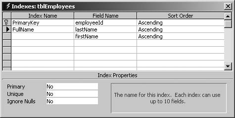
In situations where you place query criteria on multiple fields (for instance, on both lastName and firstName fields), a single compound index on those fields may run faster than separate indexes on each field. To create a compound index (see Figure 4-11), choose View → Indexes, create a new index by clicking in a blank Index Name cell (give it any name you want), and add your first field by clicking in the Field Name cell to the right and selecting the field from the drop-down menu. Add successive fields by clicking in Field Name cells in the rows below. These fields will be added to the new compound index you just created in the Index Name cell (as long as you don’t add an additional Index Name to match the additional fields; as soon as you add another Index Name, you start adding a completely new index).

Figure 4-11.  Figure 4-11. This employees table has two indexes: a primary key index on the employee ID (which prevents duplicates), and a compound or multi-field index on the first and last name fields.

Note that the order of fields in a compound index is significant; if you use the wrong order, the index won’t work at all. Use the order that fields will naturally be sorted or searched in. (MSKB 209564 discusses some significant limitations of compound indexes.)

Should you use a compound index, or separate indexes on each field? There’s no hard and fast rule. Experiment to see what gives you the best performance. You may be able to speed up your query using a compound index, but it’s not guaranteed. Try it and find out—it’s not hard to do, and you can always delete it if you don’t like the results.

In addition to indexes, there are other ways to speed up queries. Two simple things you can do are:

For more tips, go to MSDN (http://msdn.microsoft.com) and search for “Ways to optimize query performance.” The article is also included in some versions of Access Help.

THE ANNOYANCE: I created a query that generates a list of teachers and the classes they teach (see “Query Multiple Tables,” earlier in this chapter). The query is based on a join of a teachers table and a classes table. But for some reason, Access leaves out some of the teachers. What’s wrong?

Figure 4-12. The teachers table includes one teacher, Sue Levin, whose ID doesn’t appear in the classes table.

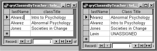
THE FIX: This isn’t an Access error, but a faulty design choice. The art of successfully joining tables involves anticipating which data doesn’t match between the two tables. For instance, in Figure 4-12, you’ll see that while Sue Levin is in the teachers table, her teacherId doesn’t appear in the classes table. When you join these two tables, you have to make a choice. Do you want teachers who have no current classes to show up in your results? Maybe not. But in some cases, you may want the unassigned teachers to show up, perhaps with “UNASSIGNED” next to their names. You can do this easily by modifying the type of join that you use. Figure 4-13 shows the two different results.

Figure 4-13. The query results on the left are based on an inner join between teachers and classes. It omits teacher Levin, because there’s no record with her teacherId in the classes table. The query on the right uses an outer join, which includes all teachers regardless of whether there are records for them in the classes table.

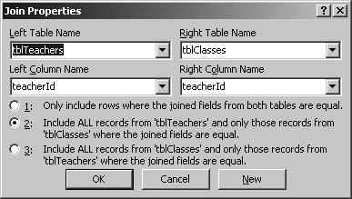
Here’s how to generate each result. In query Design View, right-click the join line that connects the two tables and select “Join Properties.” Default option 1 is “Only include rows where the joined fields from both tables are equal.” This means that rows (such as Sue Levin’s) where there’s no matching value will be omitted. (A join that omits nonmatching rows is known as an inner join.) To show all teachers regardless of any matches in the classes table (what’s known as an outer join—also termed a left or right join), you’d pick option 2 (see Figure 4-14).

Figure 4-14. To change an inner join into an outer join, right-click on the join line and open its properties dialog. The second option makes it a left join, the third option makes it a right join.

If you need nonmatching rows from both tables, see “Full Outer Joins,” later in this chapter.

When you use an outer join, you’ll often want to set up an expression to handle the null values that can arise in your results. For example, in place of className in the query design grid, use an expression like:

	Class Title: IIf(IsNull(className), "UNASSIGNED", className)

This tests the className field and, if it is null, replaces it in your query results with the text string “UNASSIGNED.”

THE ANNOYANCE: My company leases construction equipment, and I’m trying to generate a list of contracts where the closing date is after the lease date (in other words, where the rental started before the deal was signed). Simple, right? The Criteria line for my closing date field in the query is > "leaseDate“, but I get no results—and I know they’re there!

THE FIX: It’s baffling when you pull together all the pieces of a query and it comes up empty. A query can really seem like a black box—you just push the button and hope it works. Fortunately, queries aren’t black boxes: you can open them up, look inside, and figure out what’s going on. There are two things to look at: the table joins and the criteria. Save a backup copy of your query so that you can edit it without losing your original work, then start digging.

Open the query in Design View and check the items listed on the left side of the query design grid. Make sure there isn’t any “Append To,” “Update To,” or “Delete” line; those kinds of queries do not return data. If one of these lines appears, click Query → Select Query to make it a select query. Also make sure that at least one box is checked in the Show line.

If your query has joins, it’s possible that null values in your join fields are causing data to be omitted. Remove all criteria from the Criteria line in the query design grid, then switch to Datasheet View. If your data is still missing, either it’s simply not in your tables, or there’s a problem with your joins. (See “Query Multiple Tables,” earlier in this chapter, for help with joins.)

Now add back your criteria expressions one at a time. After each one, switch to Datasheet View to make sure you’re getting the data you expect. Remember that Access is strict about the way it interprets your expressions. If you tell it ="California" but your data is stored as “CA,” you won’t get a match. In your case, the problem is with the quotation marks around leaseDate, which make Access interpret the string as text. Instead, use > [leaseDate]; the brackets tell Access to interpret the string as a field name (see “[Brackets] Versus “Quotes"” in Chapter 7).

While you’re at it, look to see if the fields in the tables you’re searching have formats applied to them. (In table Design View, click the field name in the upper pane of the screen and look at the Format property listed on the General tab at the bottom.) Why does this matter? Formats only affect the way data is displayed, so they won’t affect search results. But since the data you search for may be based on the way the values are displayed, you may be confused by the results you see. For example, if you see many entries of $100 in the table, you’d expect the search criteria =100 to find those records. If none show up, it’s possible that the numbers in the table are actually $99.95, $100.03, and so on, but the format is set to round them to the nearest dollar.

If you’re using one or more “or” lines underneath the Criteria row (see Figure 4-15), there’s another gotcha. The criteria for additional fields must be repeated on every “or” line, or they will apply only to the data in the line on which they appear. You can avoid this problem by combining the separate lines into a single expression, using the OR operator to connect them. For instance, instead of putting "CA" and "NV" on separate lines, simply use "CA" OR "NV" on the first line.

Figure 4-15. Think this query finds employees who live in California or Nevada, and whose manager’s ID is 3? Nope. It finds all the employees who live in California and whose manager’s ID is 3, plus all employees who live in Nevada, regardless of their manager’s ID. The “3” must be repeated in every “or” line.

Getting expressions right is tricky, and Microsoft makes it doubly hard because Access Help barely covers the subject. You can find some examples by going to Help’s Contents tab, opening Queries → Using Criteria and Expressions to Retrieve Data, and reading the “Examples of Expressions” article. (In some versions of Access, look in Working with Expressions → Examples of Expressions.) Also see “Simple Validation Rules” in Chapter 3, and the “Expressions” section in Chapter 7.

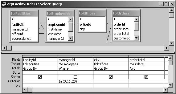
THE ANNOYANCE: I’m trying to create a totals query that shows the total payments from each of our facilities. I’m grouping on the facilityID field, and I want to include the name and address for each facility as well. But Access keeps giving me this error: “You tried to execute a query that does not include the specified expression <expr_name> as part of an aggregate function.”

THE FIX: What you’re doing makes sense, but it isn’t quite right. It makes sense because you know that for every record where the facilityID is the same, the name and address will also be the same. The problem is that Access doesn’t know this—and that’s what the error means. Those fields that don’t have an aggregate function applied to them (in other words, that don’t have anything in the Total line of the query design grid) are causing the problem. The fix in your case is easy: just set those fields to use “Group By” in the Total line. Grouping on redundant fields will cause no harm. For instance, grouping on name and address fields in this example won’t change the groups created by simply grouping on facilityID.

Sometimes, however, this fix is not appropriate. If the additional fields are not all the same within each group, and you need to use them for query criteria before any aggregate functions are applied, use the “Where” choice in the Total line, and enter the criteria below as usual—for example, total payments from facilities located only in New York, Rhode Island, and Pennsylvania. Otherwise, these fields don’t belong in a totals query, or you must apply some appropriate aggregate function to them (see Figure 4-16).

Figure 4-16. In a totals query, every field on the Total line must have a setting. This query uses a WHERE clause to restrict the search to a small set of manager IDs; then it groups on facility ID and city, and calculates the average of the order total field.

If you’re writing SQL code and getting aggregate function errors, you’re probably trying to use an aggregate function in a WHERE or GROUP BY clause. They don’t belong there; aggregate functions can be used only in clauses that apply to groups of rows (or to the entire table, if there’s no grouping). These clauses include the SELECT list, and the HAVING and ORDER BY clauses when used with GROUP BY.

THE ANNOYANCE: I have a totals query that computes an average score for every soccer team I track. But when I checked some of the averages by hand, I found Access wasn’t calculating them right!

THE FIX: If the calculations are coming out wrong, some of your records might have null values. Access will ignore those records, and that will change the average (or count, and so on) it computes. To include those records, in the Field line of the query design grid replace the field name (such as team-Score) with an expression such as Nz(teamScore). This converts null values to zeros and ensures that every record will be included in the calculation.

THE ANNOYANCE: I have a crosstab query with monthly column headings formatted as Jan-05, Feb-05, and so on. Instead of sorting the columns in date order, Access sorts them alphabetically! This is absurd.

THE FIX: Access lets you apply nice formats to dates, but then it stops treating them as dates. This is darned annoying—and the quirk isn’t limited to Date/Time fields, either. The fix involves convincing Access to interpret your sort field using the data type that you have in mind, rather than the one that it thinks it sees.

When you’re working with dates, the Format function is the usual culprit. It allows you to apply custom formats, but it returns a string value—which Access treats alphabetically. The best workaround is to omit the formatting from your query and apply it later—for instance, by using the Format property of a text box in a report. But sometimes you really need the field sorted within the query itself—say, if you’re using the query as the control source for a combo box. Often, the easiest thing to do is add another copy of your date field, uncheck the Show box, leave it unformatted, and sort on that field. But this won’t work with your crosstab column headings. If your crosstab columns must be sorted within the query, pick a date format that you can live with and that sorts correctly alphabetically (for instance, yyyy/mm/dd or yyyy-mm)…and live to fight another day.

THE ANNOYANCE: All I want is a list of my clients and any active projects they have. I joined my clients and projects tables, using a left join so I get all my clients. That works fine, except that my results include tons of inactive projects, and I only want the active ones. But when I add criteria (on the Criteria line) to filter out inactive projects on the projects side, I don’t get the full client list.

THE FIX: It’s easy to confuse how left and right joins work. When you set up your left join, you selected the option that said “Include ALL records from tblClients and only those records from tblProjects where the joined fields are equal.” You probably thought that no matter what else you defined in your query, you ought to get all of your clients. Wellll, it doesn’t quite work that way. That’s because the join gets done first, and your query criteria get applied after. Let’s look at your example.

If you look at the results of your clients/projects join before adding any criteria, you should see all of your clients. But you also may see that some clients have all nulls in the projects fields. That’s to be expected, because the whole point of the left join was to pull in all the clients, even if they don’t match anything in the projects table.

But now what happens when you set criteria such as "ACTIVE" on the project status field? Your clients that don’t have any projects at all certainly don’t have any active projects, and this test will filter them out. You can pull them back in by changing the criteria to "ACTIVE" OR Is Null. This limits your results to clients that have active projects, or no projects at all—but it doesn’t pick up clients who have only inactive projects.

To get exactly the results you want, define a separate query on your projects table, and set the criteria to "ACTIVE", as above. This pulls all active projects out of the projects table. Now, instead of adding the projects table to your main query, add this active projects query, and create your left join between clients and active projects. Your results will show all of your clients, and any active projects that they have.

THE ANNOYANCE: I created a simple query to get class registration records for our students—just three tables and two joins—and I did it all in query Design View. But when I run the query, Access says, “The SQL statement could not be executed because it contains ambiguous outer joins.” In SQL View, I get “Join expression not supported”—but Access generated the darn SQL statement, not me!

THE FIX: These errors can arise for two completely different reasons: one when Access generates the SQL, and the other when you do. If Access generated it, it means there’s an ambiguity in your use of inner and outer joins that Access can’t resolve. If you wrote it, there’s probably a problem with the ON clause of your join. We’ll look at the latter case first, because it’s simpler.

The problem with the ON clause (which occurs only if you’re writing your own SQL) can be as simple as forgetting to put parentheses around a compound condition, such as (tblTrials.trialCode = tblExp.trialCode AND tblTrials.facet = tblExp.facet). You’ll also get this message if the ON clause is incomplete or contains “too many” tables—but, of course, Microsoft doesn’t say how many is too many.

The other cause of these join errors may be ambiguous combinations of inner and outer joins in either SQL View or query Design View (see Figure 4-17). If your SQL code uses parentheses correctly, your joins are not ambiguous; the problem is that Access ignores parentheses when interpreting the order of joins! To make matters worse, Access’s error handling is ridiculous. If you’re working in the SQL window, you’ll get a “Join not supported” error when you try to save or switch back to the query design grid. But if you’re in the grid and you try to run the query, you’ll get the “ambiguous outer joins” error.

Figure 4-17. This query won’t run, because Access considers the join order to be ambiguous. The fix is to break the query into two parts, and have the first one call the second.

Consider these two joins: (A LEFT JOIN B) INNER JOIN C and A LEFT JOIN (B INNER JOIN C). In SQL, the parentheses indicate which join should be performed first—and the order matters. In the first join, the left join preserves all the rows of A, but then the inner join may discard some of them. In the second, you may lose some rows from B and C, but you’re guaranteed to get all the rows of A. The problem is that Access ignores the parentheses, and tries to interpret the SQL like this: A LEFT JOIN B INNER JOIN C. But as we’ve seen, this statement is ambiguous, because it has two different outcomes depending on which join gets executed first. It’s a real pain in the Access.

The workaround is to create a separate query that forces Access to interpret the joins in the order that you want. For example, if you want the inner join to be performed first, create a query such as B INNER JOIN C and save it as qryBC. Then recast the original query as A LEFT JOIN qryBC. This works in query Design View as well as in SQL View, since you can treat a saved query like a table in either place (see Figure 4-18).

Figure 4-18. We fixed this problem query by creating a separate query, qryFacilityOffices, which does the left join. Then we added that “subquery” to our main query and created the remaining inner join. Now Access knows to do the left join first.

THE ANNOYANCE: I added input masks to the phone, Zip Code, and Social Security Number fields in my table to make data entry easier and more accurate. The input mask seems to work properly for data entry, but queries that include these fields aren’t finding all the records.

THE FIX: Input masks are a handy way to force users to enter data in a fixed format. For example, to prevent users from entering phone numbers in a mix of styles, such as (413) 222-1111, 413-222-1111, and 413.222.1111, you can give them a data entry form like the one shown in Figure 4-19. But if you store mask characters such as parentheses or hyphens in your data (or conversely, only use them for display) and your query doesn’t reflect this, you’ll get just the problem you describe.

Figure 4-19. An input mask for the phone field automatically presents the user with parentheses and a hyphen, and allows only numbers to be entered.

When you create an input mask, the value following the first semicolon specifies whether to store the mask characters in the table or not: 0 means store mask characters, and 1 means don’t store them. For example, with an Input Mask property setting of (000") "000-0000;0;_, the value stored in the table will be (413) 222-1111. With an Input Mask setting of (000") "000-0000;1;_ or (000") "000-0000;;_, the value stored will be 4132221111. The problem, of course, is that it’s easy to forget which you’ve chosen, since the formatting appears in forms and datasheets with no indication of what’s stored in the field.

Because queries search the underlying data, not the formatted values, your query criteria must precisely match the way the values are stored (with or without mask characters, in this case). The problem gets worse if you add an input mask to a table that already contains data: Access doesn’t update the existing records, so older values might be stored with formatting, while newer ones are not. For this reason, we recommend that input masks be applied at the form level rather than at the table level. That way, you can see exactly what’s in your table.

If you’ve already applied a mask at the table level, here’s what to do:

THE ANNOYANCE: I have a simple parameter query that lets users input a phone number and receive any matching records. But I can’t figure out how to make the query use wildcards.

THE FIX: The trick is using the Like operator. (It’s hard to find, but the Like operator is documented in Help: see Microsoft Jet SQL Reference → Overview → SQL Expressions. (In Access 2000, on the Index tab, search for “Like.”) If you want users to enter the wildcard characters, put Like [Enter phone number] in the Criteria line of the phone number field. If a user enters 212*, she’ll get all the phone numbers that begin with 212. Enter # to match any single digit, and ? to match any single alphanumeric character. For instance, entering 21#-323-4100 returns 210-323-4100, 211-323-4100, and so on.

If you don’t want users to enter wildcards, enter criteria such as Like "*" & [Enter phone number] & "*". Adding the wildcard to both ends of the input string ensures that your query will automatically return all matches. For instance, if a user enters 212-432, he’ll get back any phone numbers that contain those digits, such as 212-432-3323 and 441-212-4324.

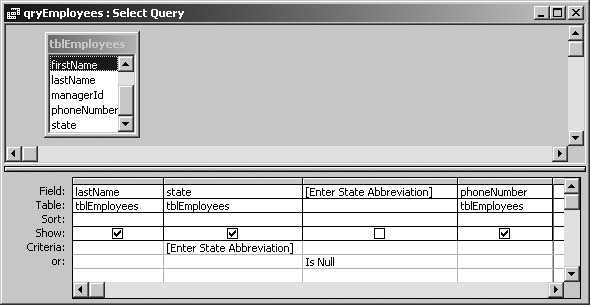
THE ANNOYANCE: I have a simple parameter query that accepts a state abbreviation and returns matching records. If users leave the parameter blank, I’d like it to return all records, but I can’t make this work.

Queries That Accept Parameters

You’ve just a designed a wonderful query that shows sales data for the past year. There’s only one problem: your users don’t always want a year’s worth of data. Sometimes they want the data from a three-month period, say, or for six months starting in the second quarter of the previous year. Making a separate query for each scenario is way too much work, though, and creates maintenance problems.

That’s why Access lets you use parameters in your queries. A parameter is simply a variable. When you run the query, it prompts you to provide a value for the variable, and then the query runs based on that value. For instance, instead of hard-coding dates into your sales query, you could provide start date and end date parameters and let users specify the date range when the query runs.

Access makes it easy to specify parameters. Anything that looks like a field name (namely, anything in brackets) that Access can’t locate in your tables is treated as a parameter. For example, if you put [CustName] on the Criteria line in the query design grid, when the query runs Access will prompt you for a value, and then use it as query criteria for that field. (When you want a parameter, this is great; if you don’t, and you see the parameter dialog box, it’s really an error message. See “Enter Parameter Value” in Chapter 1.) A common trick is to name parameters something like [Last name of customer?], which makes the “Enter Parameter Value” prompt a bit more user-friendly (see Figure 4-20).

Figure 4-20. When you use a query parameter, Access presents the parameter name as part of the input prompt. For user-friendliness, use a name like “Last name of customer?” rather than “CustName.”

In certain cases—crosstab or action queries, queries that underlie charts, criteria for Yes/No fields, and fields in external databases—you must declare the data type of the parameter. In query Design View, choose Query → Parameters and fill in the name (e.g., [Last name of customer?]) and data type, such as Text or Integer. Even when it’s not required, it’s good practice to specify parameter data types for anything other than text. That way, users who enter invalid data will get a reasonably sensible error message; if you don’t, they’ll get pure gobbledygook (see Figure 4-21).

Figure 4-21. Two different error messages when a user enters invalid data for a parameter. If you specified the data type, users will get the pleasant message above. If you didn’t, they’ll get the forbidding one below.

THE FIX: When the parameter prompt is left blank, its value is null. Since null values require their own tests (see “Tangled Up in Null” in Chapter 7), you’ll need to add query criteria so Access can handle this situation. For example, to return all records, put something like [Enter state abbreviation] Or [Enter state abbreviation] Is Null on the Criteria line in the query design grid (see Figure 4-22). Because an Or statement is true if either condition is true, if the parameter comes back null, every record will satisfy this criterion. This technique also works with Like statements and Between … And criteria.

Figure 4-22. To include all records when the parameter is left blank, add the Is Null test as an alternative Criteria row.

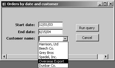
THE ANNOYANCE: Our sales database has a massive amount of information in it, and I need to give users the ability to select data by specifying multiple parameters, such as date range and region of interest, and so on. But Access’s built-in query parameters are far too simple to handle this task.

THE FIX: No kidding. Access’s built-in parameters are useful if you need, say, data from a single date, but not for much more. If there’s more than one parameter, the prompts come one after another, rather than all on one page, and there’s no way to add error handling, drop-down lists, or other conveniences to make parameter entry more user-friendly and reliable. Fortunately, you can do all this (and more) with forms—and it’s easy to use form data as parameters for queries.

First, create an unbound form (see “Create Dialog Box Input Forms” in Chapter 5) and add the controls that you’ll need for user input (see Figure 4-23). Use text boxes for free-form data entry, combo and list boxes to constrain users to predefined values, and any other controls you need. All the usual “good design” practices apply, so use format and validation rules where appropriate to help your users submit valid parameters. Don’t forget to add a “Run query” button.

Figure 4-23. A simple unbound form lets you gather user input on which you can base the query criteria. It’s far friendlier than “Enter Parameter Value” boxes.

Once the form is complete, you can reference its data in your query by placing fully qualified control names such as Forms!frmMyParamForm!txtMyParamField on the Criteria line of your query. (“Fully qualified” simply means using the whole path, not just the short name; in this example, txtMy-ParamField is the short name.) Here, frmMyParamForm is the name of your unbound form, and txtMyParamField is the name of a field on that form. For example, to use a date range as a query criterion, you’d enter something like Between Forms!frmMyParamForm!txtStartDate And Forms!frmMyParamForm!txtEndDate on the Criteria line of your query. When the user hits the “Run query” button, the query will pull those values (namely, the start and end dates she’s entered in the form) from the data entry form. If your data entry form uses a combo box rather than a text box, you can use its value, like this: Forms!frmMyParamForm!cboMyComboBox. The usual rules about declaring parameter data types apply here. (See the sidebar "Queries That Accept Parameters,” earlier in this chapter.)

In order for this to work, the form must be open, with the date range already entered, when the query is run. (If it isn’t, Access won’t be able to resolve the control names and will resort to the “Enter Parameter Value” prompt. You don’t want that.) The simplest way to ensure this is to put the “Run query” button on the form itself. You can use the Command Button Wizard to do this (see “Activating the Wizards” in Chapter 5). Once the wizard starts, choose the Run Query action in the Miscellaneous category on its first page.

THE ANNOYANCE: I want to create a parameter query that computes sales statistics for a set of cities. I built an input form (as described in the previous Annoyance) with a nice list of cities for users to choose from, but there seems to be no way to get the list into my query!

THE FIX: Letting users choose from a parameter list makes sense, but alas, Access doesn’t support this very well. There are a couple of workarounds, but neither one is completely satisfactory. The first solution is relatively easy, but it sticks the user with a crude user interface (manually entering a comma-separated list of parameters). The better solution uses a multi-select list box, but this requires writing some VB code. Figure 4-24 shows both alternatives.

Figure 4-24. Two different ways to enable users to input parameter lists. In the above approach, which is much more error-prone, the user must enter a comma-separated list. The multi-select list box below is far more user-friendly.

If you don’t mind asking your users to type in a comma-separated list (as opposed to choosing from a list), you can use the first approach. On the Field line of your query grid, put [Enter city or list of cities], and on its Criteria line, put Like "*" & [ cityField ] & "*" (where cityField is the field that contains the city names). This is the opposite of how you usually use the Like operator—instead of saying cityField LIKE "Boston", we’re saying "Boston, New York, Springfield" Like *cityField*. Adding wildcards to the field value ensures that each city will match when compared to the whole list.

This works fine with some data being queried, but in other situations the wildcards may yield false hits. For instance, a user who searches for Dayton will retrieve both Dayton and Daytona Beach. To prevent this, add a delimiter such as a comma to your expression. For example, type "," & [Enter city or list of cities] & "," on the Field line, and Like "*," & [cityField] & ",*" on the Criteria line. This forces the query to match the entire field. However, the match will fail if the user enters a space after the comma by accident—a common mistake. Change the criteria to Like "*[, ]" & [cityField] & "[, ]*", and it should work. (Remember that brackets inside quotes are not defining a field name, they’re defining a character set—in other words, telling Access to match both comma and/or space.)

For most users, a multi-select list box on an unbound input form is a far better choice; there’s no fussing with commas and no risk of misspelling a name. Though you’re probably more familiar with combo boxes, list box controls are very similar and have a similar wizard. (If you’re unsure of how to use an unbound input form, see the previous Annoyance, “User-Friendly Parameter Queries.”) To make this fix work, though, you’ll need to write a bit of VB code.

By default, list boxes have their Multi Select property—which allows a user to make multiple selections—set to “None.” From the Other tab in the list box’s properties sheet, change this to “Simple” or “Extended,” depending on which style of multiple selection you prefer.

The problem now is that there’s no easy way to get the user’s selections back into your query from your form; you need a bit of VB code to loop through the selections and construct a criteria string. Run Access’s VB Editor, pop in this code, save it, and tie it to the OK button’s Click event:

	Dim varItem As Variant
	Dim strInClause As String
	If Me!lstCities.ItemsSelected.Count = 0 Then
	    MsgBox("Please select at least one city.")
	Else
	    strInClause = "[city] IN("
	    For Each varItem In Me!lstCities.ItemsSelected
	        strInClause = strInClause & """" & _
	            Me!lstCities.Column(0,varItem) & """" & ", "
	    Next varItem
	    'Remove the trailing comma and space from the last item
	    strInClause=left(strInClause,len(strInClause)-2) & ")"
	End If

	[PAGE 197]
	Private Sub Form_Current()
	    If IsLoaded("frmInvoices") Then
	        Forms!frmInvoices.Filter = _
	                 "ClientID = Forms!frmClients!ClientID"
	        Forms!frmInvoices.FilterOn = True
	    End If
	End Sub

This code starts with the string fragment "[city] IN(“, and then builds up the list of cities for the IN clause by looping through the ItemsSelected collection, which provides a list of the selected rows. In this example we use the Column property to extract column 0 (the first column) for each row, but you can extract any column. Also, note that the Column property’s arguments are the reverse of what we usually expect: (col, row) instead of (row, col).

Once you’ve created this string—which in this case looks something like [city] IN("Boston", "New York City", "Geneva")—you can use it as a filter criterion applied to a form or report. For example, to open a report with this criterion, use DoCmd.OpenReport "rptSalesSummary", acViewPreview, , strInClause. If you need to open a query, as in this Annoyance, construct the entire SQL string and use CreateQueryDef, like this:

	Dim qdf As QueryDef
	Set qdf = CurrentDb.CreateQueryDef("qrySales", _
	             "Select * From tblSales Where " & strInClause & ";")
	DoCmd.OpenQuery "qrySales"

THE ANNOYANCE: I have a crosstab query that displays suppliers by product category, and I want to let users filter the output by region. But when I try to add a region parameter to the query, Jet says it can’t recognize the field name. I can add parameters to other queries without any problem.

THE FIX: If Access doesn’t recognize something in the query design grid, it usually assumes it’s a parameter. But with crosstabs, the rules are changed: if you want to use parameters, you must declare them explicitly. Choose Query → Parameters, fill in the same parameter name that you used in your query (e.g., [Enter region]), and specify its data type (see Figure 4-25). Note that if your crosstab query is based on any other queries, parameters in those queries must also be declared.

Figure 4-25. The Query Parameters dialog lets you explicitly specify the parameter data type. You must do this for certain types of queries (such as crosstabs and action queries) and certain data types (such as Yes/No fields), but it’s good practice to do it for all your parameters.

THE ANNOYANCE: I have a crosstab query that shows accident data. The rows represent different facilities, and the column headings are teams at each facility. I want to sort the facilities by the total number of accidents (showing the most accidents at the top), but Access gives me an error when I try to do this.

THE FIX: If you’ve survived the rigors of the Crosstab Query Wizard and have actually produced a working crosstab query… congratulations! Presumably, you then opened it up in Design View and tried to set the Sort line on one of your totals fields to sort the output (ascending or descending). This sounds simple, but when you try it Access spits out an error—and for good reason.

Crosstab Traffic

When working with data, you often want to see how two different variables are related. For instance, you might want to see sales data broken out by customer and by quarter, or student enrollment by region and by family income. This kind of analysis is called cross-tabulation, or crosstab for short. One variable spans the columns while the other variable goes down the rows, producing a rich cull of information.

Access has a Crosstab Query Wizard (Insert → Query) that makes it easy to create crosstabs. If all the data you’ll need is in a single table, you can apply the wizard to that table; otherwise, you’ll need to combine the data from multiple tables into a single query first (see “Query Multiple Tables,” earlier in this chapter) and base the crosstab on that. When the wizard asks you to specify row headings, it’s asking which field in your table will provide the headings for each row. In Figure 4-26, that’s company name. Next, the wizard asks for the field that will supply “column headings” along the top of the query; in this example, that’s the order date. Since this column heading is a date field, Access asks if you want to group dates into units such as years, quarters, or months. (As you can see in Figure 4-26, we said yes to quarters.)

Next, the wizard asks what number should appear at each row/column intersection. That’s because, in a typical crosstab query, you’ll have more than one data item at each intersection. For instance, in our sales crosstab, each customer might have multiple orders in a given quarter. You might want to display the average, maximum, sum, and so forth. We chose sum. On the same page, you can add a summary column (the Total Orders column) that totals the figures for each row (as in Figure 4-26).

Figure 4-26. A crosstab query allows you to view your data using multiple factors at the same time. In this example, order totals are broken out by company name and by fiscal quarter.

Access doesn’t support this feature! (Of course, you can reference an aggregate column alias, such as a Count of Accidents in SQL using the ORDER BY clause, but Access SQL won’t do it.) The workaround is to base a new query on your crosstab query, and do the sort there. Here are the steps:

THE ANNOYANCE: I’m designing a crosstab query to summarize sales data for different offices over the past 12 months. I want to display more than one aggregate statistic at the intersection of each row and column, but I can’t figure out how.

THE FIX: PivotTables were invented to solve this very problem. A PivotTable is a dynamic, interactive table—really, a kind of report—that lets you explore different views of complex data. A powerful alternative to static reports, PivotTables allow you to quickly see “what if” without modifying the underlying data. PivotTables aren’t updatable, which means you can play with them without worrying about messing up your data. They can’t be used for data entry, but they’re a very valuable tool for interactive data analysis. PivotTables have been available for years in Excel and were first introduced in Access 2002. If you’re using an older version of Access, we discuss some alternatives at the end of this fix.

PivotTables (and PivotCharts) are complex beasts; we won’t tackle them here. But to get a feel for their capabilities, try this: open the table (or query) that your crosstab is based on in Datasheet View, and then select View → PivotTable View. You should see a PivotTable field list. (If not, select View → Field List.) Now drag the row and column fields and drop them into the places reserved for them (you’ll see labels such as “Drop Row Fields Here”), as if you were manually creating your crosstab. (If you’re looking at a blank screen, see MSKB 307905 for the bug fix.)

This creates your framework. Populate the framework by dragging other fields into the areas marked for them (see Figure 4-27). To apply an aggregate function, right-click the field name in the column heading and choose “AutoCalc.” To show only the aggregate values, right-click the column and choose “Hide Details.” You control everything via the PivotTable menu and by right-clicking. The trickiest part of the interface is that there’s no way to throw away your work and start over—not even by quitting (because you’re defining a view, and Access remembers it)—and sometimes it’s not obvious how to return to an earlier view. However, you can always right-click your row and column headers, and select “Remove.” This empties your PivotTable so you can start over.

Figure 4-27. This PivotTable view of the orders table was generated with just a few clicks—dragging customer ID to the “Drop Row Fields Here” area and order date to the “Drop Column Fields Here” area. The grand totals were created by clicking the plus sign under Grand Total and then right-clicking and choosing AutoCalcSum.

If you’re using Access 2000 or an earlier version, or you don’t want to use a PivotTable, there are a few tricks that let you display multiple values in a crosstab. By design, a crosstab can have only one Value column in the query grid, but you can combine multiple aggregate values in a single column. For example, an expression such as Sales Avg and Sum: Avg(sales) & "/" & Sum(sales) would give you both average and total values, concatenated into a single string: $5,770/$48,908. (The first term is the average; the second term is the sum.) Of course, if you need to use these values in a report, you’ll have to write some code to parse them back out. Another workaround is to create a separate crosstab query for each value that you want, and then join those crosstabs into a third query, arranging the fields as you wish. (See MSKB 209143 for details.)

THE ANNOYANCE: I need to generate a list of all my projects whose dates overlap with other projects going on in the same city. All this info is in my projects table, but when I try to create a query that compares different rows, it doesn’t work. Are Access queries truly limited to looking at one row at a time?

THE FIX: Like every relational database, Access is row-oriented. When you set criteria in a query, those criteria get applied one row at a time—not across different rows. But to compare the date ranges of different projects, you must examine pairs of rows at the same time. It seems impossible in Access, until you know the trick.

Since you can’t change Access’s one-row-at-a-time mentality, create a virtual table that has the information you need in each row. You’ll do this using a join (see “Query Multiple Tables,” earlier in this chapter). Since you must look at each project paired with every other project, add the projects table to the query Design View window twice. Adding the same table to a query more than once is known as a self-join.

Notice that Access adds “_1” to the name of the second copy. This lets Access distinguish which field you’re referring to when you add fields to the query design grid, since otherwise, the fields in both tables would have identical names. For example, if you add the project title field from each table, Access will represent them as tblProjects. projectTitle and tblProjects_1.pro-jectTitle. You’d be well advised to give them more meaningful names, such as Project 1: tblProjects.projectTitle and Project 2: tblProjects_1.projectTitle.

With no join lines between the two copies of the table, Access generates a list combining every row with every other row (see Figure 4-28). To include only rows where projects are in the same city, join on the city field. (It’s a good idea to join on the state field, too, to avoid mix-ups with identically named cities in different states.)

Figure 4-28. When you add two copies of the same table to a query, you start out with all possible pairs of rows in the two tables, including each row paired with itself. Use join lines and criteria to restrict which rows remain in the query.

Now add the fields that you want in the results (project title, city, state, and so on), and you get Figure 4-29.

Figure 4-29. The final query, which detects date range overlaps, is not complicated—but getting the details right is tricky.

The hardest part of this query is picking the criteria that will detect a date range overlap. (See “Dates! Dates! Dates!” in Chapter 7 for full details.) You can start by adding tblProjects. startDate to the grid, and in its Criteria line adding < tblProjects_1.endDate. Then add tblProjects.endDate, and in its Criteria line put < tblProjects_1.startDate. In other words, Project A overlaps with Project B if A’s start date comes before B’s end date and A’s end date comes after B’s start date.

This works great, except that every pair of overlapping projects appears in the results twice. That’s because the criteria are symmetrical: if Project A overlaps Project B, then Project B overlaps Project A, so the results include both row orderings. And since every project overlaps itself, these show up as well. To exclude these redundant rows, add tblProjects.projectId to the query design grid, and set its Criteria line to < [tblProjects_1].[projectId]. This may seem like an odd addition, since whether a project’s ID is less than any other project’s ID is totally arbitrary. However, this trick excludes self-matches, and it (arbitrarily) eliminates one of the redundant entries in each pair.

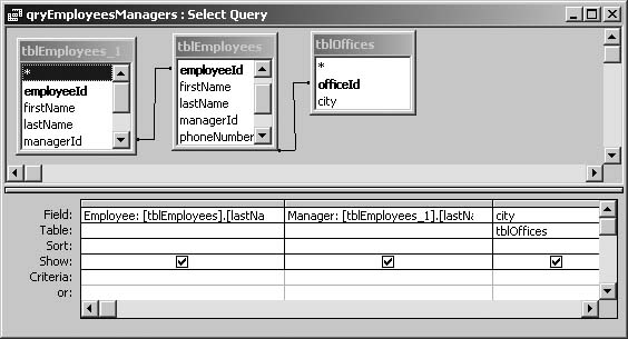
THE ANNOYANCE: We have a managerId field in our employees table that points to the manager for each employee. But data on managers is also stored in the employees table. How can I generate a list of employees with the appropriate manager’s name next to each employee?

THE FIX: When a foreign key (see “Relationship Angst” in Chapter 3) refers back to its own table, it creates a type of relationship that is useful for representing trees and hierarchies. The classic example is managers and employees, where managers are employees whose IDs show up in other employees’ managerId fields. This type of recursive relationship can nest within itself an arbitrary number of times (managers who have managers who have managers, and so on).

In the days before the advent of relational databases, hierarchical database systems ruled the roost, and they made it easy to work with these kinds of data. But relational databases are not optimized to work with trees or hierarchies, and there’s a limit to what you can do without creating some kind of procedural code (whether stored procedures or application code) that reconstructs the hierarchy from the raw data. In this fix, we’ll stick to the basics.

To show a list of employees and their supervisors, use a self-join (see the previous Annoyance, “Comparing Different Rows”). Add two copies of the employees table to the query Design View window, and drag the managerId field from the first copy onto the employeeId field from the second (see Figure 4-30). The first copy of the table will contribute employee names, while the second will add their managers. If you want to include employees who don’t have managers, turn this join into an outer join by right-clicking the join line, choosing “Join Properties,” and then choosing option 2 (“Include ALL records from ‘tblEmployees’ etc.”).

Figure 4-30. This query uses a self-join on the employees table on employeeId, as well as a simple join on the offices table on officeId. The employee names come from tblEmployees, and the manager names come from tblEmployees_1.

Self-joins are not limited to only two copies. If you need to show the managers of the managers, you can do it by repeating this process and adding a third copy of the table to the query Design View, and so on for more levels. Note, however, that if you don’t know in advance how deep your org chart is, there’s no good way to finish the problem—that is, to show the complete hierarchy—using this approach. For a general solution, you must add procedural code.

Still, there are a few other questions that are readily solved with this design. To find the big boss(es), look for employees with nulls in the managerId field. To find the employees who don’t manage anyone, use a subquery (see “Divide and Conquer with Subqueries,” later in this chapter):

	SELECT *
	FROM tblEmployees As e1
	WHERE NOT EXISTS
	    (SELECT *
	    FROM tblEmployees As e2
	    WHERE e1.employeeId = e2.managerId)

THE ANNOYANCE: I need a report that summarizes our purchase orders, broken into groups based on the size of the order. What I can’t figure out is how to create groups based on ranges such as $0 to $100, $101 to $500, and so on.

THE FIX: When you want to create groups, you need a grouping field—in other words, a field whose value will be the same for every row in the group. There are two different ways to do this: using an expression or an auxiliary table. An expression offers more flexibility, but the auxiliary table performs faster.

To use an expression, you need a function that maps each range into a constant value. You’ll add this function to the Field line of the query design grid, and then group on it. The built-in Partition function, which slices a range into fixed categories, is intended for just this purpose, but unfortunately it’s not flexible enough to be very useful. For simple cases, the Switch function is usually a better choice. For example:

	AmountRange: Switch([orderTotal] Between 0 And 100, "$0 to $100",
	[orderTotal] Between 101 And 500, "$101 to $500", [orderTotal] Between 
	501 And 5000, "$501 to $5000")

The Switch function evaluates every range expression (Between…And) and returns the label associated with the one that is found to be true. For example, all order totals less than $101 will be mapped to the AmountRange “$0 to $100” (the Between…And operator includes both ends of the range). Now you can group on the AmountRange expression. Pay attention to the points where your ranges meet. They shouldn’t overlap, but you don’t want values falling between the cracks, either. Sometimes it’s easier to specify conditions explicitly, like this: [orderTotal] >= 100 AND [orderTotal] < 500.

For more complex conditions (say, orders that are less than $101 and come from the West Coast), the Switch function is unwieldy. Instead, define your own Visual Basic function, save it in a module, and call it from your query with whatever input you need, like this: AmountRange: createOrderPartitio n([orderTotal], [postalCode]). This function should accept any order total and postal code and return a range label that allows the query to put it into a group.

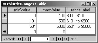
A different approach to creating ranges is to add an auxiliary table to your query. A typical range table has three fields: minValue, maxValue, and rangeLabel (see Figure 4-31).

Figure 4-31. A simple range table defines ranges and provides a text label for each range.

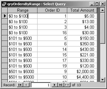
Add this table to the query Design View window, but don’t create a join. Add the rangeLabel field to the query, and in its Criteria line put something like [orderTotal]>=[minValue] And [orderTotal]<[maxValue]. Group on the range-Label field. Figure 4-32 shows the result before you group on rangeLabel, and Figure 4-33 shows the result after grouping.

Figure 4-32. Regardless of whether you use an expression or a range table, the effect is to add a range field to your query that is the same for every row that falls in the range. This gives you a field that you can group on to create a summary query.

Figure 4-33. Once you have established a grouping field, you can create a totals query that provides summary statistics based on that grouping.

If you are writing SQL code, note that the standard way to express this query is using a join expression, like this:

	tblOrders As t INNER JOIN tblOrderRanges As tor
	ON t.orderTotal >= tor.minValue AND t.orderTotal < tor.maxValue

THE ANNOYANCE: I’m joining two tables: publishers and articles. Some publishers have no associated articles, and some articles have no publishers, but I need them all to appear in my results. Why doesn’t Access support a full outer join?

THE FIX: Access doesn’t fully support the SQL-92 standard—not in SQL View, and not even when you’ve enabled SQL-92 syntax. It would be handy if it did, since full outer joins preserve both sides (left and right) of the join, whether there’s a matching row on the other side or not. The most straightforward workaround is to create a UNION query, combining left and right joins. This can be done only in SQL View, and the result isn’t updatable. The code (which you’d run from your query’s SQL View) would look something like this:

	SELECT * FROM tblPublishers LEFT JOIN tblArticles
	ON tblPublishers.publisherId = tblArticles.publisherId
	UNION
	SELECT * FROM tblPublishers RIGHT JOIN tblArticles
	ON tblPublishers.publisherId = tblArticles.publisherId

You might think this would produce a lot of duplicate rows, but UNION automatically removes them. To retain every row, use UNION ALL.

THE ANNOYANCE: I’m trying to find the names of all staffers who live in the same town as any one of our vendors. We have a staff table and a vendors table, but I can’t figure out how to join them to get this result.

THE FIX: Many queries don’t yield to an all-at-once solution, but if you break the problem into parts you can then piece together for the desired result. For example, if you were solving the above problem by hand, you’d probably start by writing down a list of all the vendors’ towns. Do the equivalent in Access by creating a query that finds the unique cities in the vendors table. Now add that query, along with the staff table, to a new query, and create a simple join on the cities field. Set the query’s Unique Values property to “Yes,” and you’re done.

This divide-and-conquer approach is best implemented using a subquery— a query embedded in another query. In Access, subqueries can only be created using SQL. For the example above, we could simply have said:

	SELECT DISTINCT fullName, city
	FROM tblStaff
	WHERE city IN
	    (SELECT DISTINCT city
	     FROM tblVendors);

The (SELECT DISTINCT city FROM tblVendors) part is the subquery. The subquery says, “Give me a list of the cities that are in the vendors table,” and the main query says, “Give me just the staffers whose cities are on that list.” Subqueries are often used with the IN, EXISTS, ANY, and ALL operators, in addition to the simple comparison operators. Here are a few examples:

THE ANNOYANCE: Our satellite offices submit monthly transaction reports that get recorded in a transaction reports table (tblTransactionReports). I’m trying to generate a list of offices with missing reports, but it doesn’t seem possible.

THE FIX: In a relational database, it’s easy to test for fields with missing data, but it’s impossible to directly test for missing rows. Since they’re not there, there’s nothing to select on. If you manually added a row to the reports table every month for every office, and simply left the date submitted field blank if the report was never submitted, it would be easy; you could just test for null values in that field. But that’s a lot of extra work, and there’s a better way: let Access generate your list of expected reports. This is both easier and less error-prone, and once you have that list, it’s a simple matter to write a query that combines it with your actual table to see what’s missing. Here are the steps.

THE ANNOYANCE: I need to generate monthly patient counts, based on the fiscal calendar that the hospital uses. In addition, I’m supposed to create a separate report to count how many patients show up on holidays. All I have to work with are the raw dates from the patient visits table, and I’m at a complete loss.

THE FIX: Calendars are beasts; only idiot savants really understand them. Don’t tackle problems like this with complicated date expressions—let the database do the work for you. The trick is to create an auxiliary table that has the calendar information you need (see Figure 4-35). Set up this calendar table once, and you’ll never have to worry about it again. (If for some reason—say, you’re extremely short on storage space—you do need to use an approach based on date expressions, see MSKB 132101.)

If you need only a small date range, you can set up the calendar table by hand, but if you want years’ worth of rows, create it via VB code.

Figure 4-35. A typical calendar table. By simply storing the calendar information in a readily usable format, you avoid the agony of computing date relationships using expressions within queries.

You’ll need to create the calendar table (tblCalendar) first, with all its necessary fields. Then copy this code into any module, and customize it for your needs. The following code (createCalendar) supplies the fiscal month and year, as well as a Yes/No field indicating workdays:

	Public Sub createCalendar(dateStart As Date, dateEnd As Date, _
	    intFirstFYMonth As Integer, intFirstFYDayOfMonth As Integer )
	    Dim rst As ADODB.Recordset
	    Set rst = New ADODB.Recordset
	    rst.Open "tblCalendar", CurrentProject.Connection, adOpenKeyset, _
	    adLockOptimistic, adCmdTableDirect

	    Dim lngNumDays As Long
	    lngNumDays = DateDiff("d", dateStart, dateEnd)

	    Dim dateNext As Date
	    Dim lngCnt As Long
	    Dim intMonthNext As Integer
	    Dim intDayOfMonthNext As Integer
	    Dim intYearNext As Integer
	    Dim intFiscalYear As Integer
	    Dim intFiscalMonth As Integer
	    Dim DateCurrentFYStart As Date
	    Dim boolWorkDay
	
	    For lngCnt = 0 To lngNumDays
	             dateNext = DateAdd("d", lngCnt, dateStart)
	             intMonthNext = Month(dateNext)
	             intDayOfMonthNext = Day(dateNext)
	             intYearNext = Year(dateNext)
	             DateCurrentFYStart = DateSerial(intYearNext, _
	                      intFirstFYMonth, intFirstFYDayOfMonth)

	             'COMPUTE FISCAL YEAR
	             If dateNext < DateCurrentFYStart Then
	                     intFiscalYear = intYearNext - 1
	             Else
	                     intFiscalYear = intYearNext
	             End If

	             'COMPUTE FISCAL MONTH
	             If intDayOfMonthNext < intFirstFYDayOfMonth Then
	                     intFiscalMonth = intMonthNext - 1
	                     If intFiscalMonth = 0 Then
	                             intFiscalMonth = 12
	                     End If
	             Else
	                     intFiscalMonth = intMonthNext
	             End If
	
	             'COMPUTE WORKDAY
	             If DatePart("w", dateNext, vbMonday) > 5 Then
	                     boolWorkDay = False
	             Else
	                     boolWorkDay = True
	             End If
	            'WRITE TABLE
	            With rst
	                    .AddNew
	                    .Fields("calendarDate") = dateNext
	                    .Fields("dayOfYear") = DatePart("y", dateNext)
	                    .Fields("fiscalMonth") = intFiscalMonth
	                    .Fields("fiscalYear") = intFiscalYear
	                    .Fields("isWorkDay") = boolWorkDay
	                    .Update
	            End With
	    Next lngCnt
	End Sub

To populate your calendar table with data, run the createCalendar code from the Immediate window of the VB Editor. For instance, to populate your table from June 2004 to June 2010, with a fiscal year that starts on September 15, call it like this:

	createCalendar #2004-06-01#, #2010-06-01#, 9, 15

Note that this routine doesn’t populate the isHoliday field. Since holidays are so irregular, you’ll have to add that information by hand. Also note that it does populate a day of year field (for example, October 10 is the 284th day of the year), even though this is easily computed on the fly using DatePart— summoning this information from a table is faster than recomputing it every time you need it.

To use a calendar table, you’ll typically join to it on its date field. For instance, you’d add it to your query of patient counts by joining the calendarDate field in tblCalendar to the visitDate field in the tblVisits table (see Figure 4-36). Now add tblCalendar’s fiscal month field to the query design grid, and set its Total line to “Group By.” Instead of grouping by calendar month, you’re now grouping by fiscal month—it’s as easy as that. To exclude holidays, add the isHoliday field and set its Criteria line to “False.”

Figure 4-36. You can easily create a query that groups on fiscal month and year by joining the visits table’s visitDate field to the calendar table’s calendarDate field.

THE ANNOYANCE: My old MySQL database let me use a CASE expression to create meaningful output in queries. For instance, in a query of student test scores, I could set it up so that scores greater than 90 showed up as As, and so on. But Access doesn’t support CASE.

THE FIX: Like most database systems, Access supports only a subset of ANSI SQL-92—and CASE is one of the glaring omissions. Let’s take a look at how you can (sometimes) jury-rig Access to more or less deliver the same functionality as CASE and some other missing SQL expressions: