
Neural Calculus
Abstract
A stable information theory of neural computation was introduced. It was suggested that this theory might be consistent with how learning of memory weights could be produced in neural models of dynamic spiking. It was noted that these models essentially have the same quantitative components as RELR including fast graded potentials built from polynomial terms to the fourth degree, interaction terms, and slower recovery currents that have similar properties as RELR's posterior memory weights which become prior weights in future learning. It was also noted that RELR's ability to learn patterns in very small samples of observations based upon very high-dimensional candidate features could be similar to what occurs in neurons. The crux of the analogy between RELR and learning at an individual neural level is that just as RELR's positive and negative error probabilities are equal without bias, a similar likely error and bias cancellation is expected in neurons when graded potentials sum to produce binary spiking outputs. RELR was also contrasted with widely known neural network algorithms from the 1980s. The one method from the 1980s that RELR more closely resembles is neural Darwinism, although RELR does not require a random search and thus produces more stable and more rapid solutions. It was also noted that RELR is better viewed as a neural ensemble model that reflects a “modal neuron” from a population of neurons as compared to a neural network model.
Keywords
Axon; Back propagation; Binary spikes; Boltzmann machine; Cell body; Dendrite; Explicit RELR; Genetic algorithm; Graded potentials; Hebbian learning; Hidden units; High-dimensional learning; Hopfield network; Implicit RELR; Integrate-and-fire; Interactive learning; K-means cluster analysis; Local field potentials; Multilayer perceptron; Natural selection; Neural Darwinism; Neural impulse; Neuron; Principal components analysis; Resonance; Restricted Boltzmann machine; Self-organized map; Simple model of neural dynamics; Small sample size learning; Spike-timing-dependent plasticity; Supervised learning; Synapse; Theory of neuronal group selection; Unsupervised learning
“[Neurons] are small, globular, and irregular… [and] supplied with numerous protoplasmic prolongations [dendrites]. The special character of these cells is the striking arrangement of their nerve filament [axon], which arises from the cell body …”
Santiago Ramón y Cajal, Estructura de los centros nerviosos de las aves, 1888.1
Contents
Just as the existence of atoms had been doubted through much of the nineteenth century, most scientists also did not believe in neurons in those years. Prior to the work of Cajal, the prevailing view promoted by Golgi was that the nervous system was continuously connected without discrete components through a mesh of fibers called the reticulum.2 While Cajal's discovery of neurons as discrete units that are connected through synapses has had profound effects in medical and pharmaceutical applications, it really has not yet had much effect in everyday predictive analytic applications of machine learning. Most of today's most widely used machine learning methods to model and predict human behavior outcomes, including the popular multilayer back propagation supervised artificial neural networks, do not seem to have a strong connection to real neurons especially given what we now know about how neurons work. This is similar to how alchemy had no connection to atoms.
Leibniz's goal to find a Calculus Ratiocinator has turned out to be a very difficult problem due to all the possible arbitrary ways that analytics can be generated to predict and explain complex human behavior-related outcomes. We could rely upon pure statistical theory to avoid arbitrary features. But our solution would be just a theoretical mathematical solution that may not reflect any natural mechanism that actually produces cognition and behavior. Statistical theory also has limitations as underlying assumptions may not be correct. But if the supposed nonarbitrary statistical properties are also seen in neurons, then there will be better chances of being on the right track. RELR does provide a feasible solution grounded in statistical theory that that has important computational features that are also seen in neurons.
Obviously, RELR is not the first attempt to base a predictive analytic method upon neuroscience as the artificial neural networks that were introduced in the 1980s made that attempt. Also, RELR is not the first proposal that the neuron is essentially a probability estimation computer constantly predicting its own maximum probability output.3 What then is different about RELR's modeling of computations at the neural level? First and most importantly, the error probability modeling that is the basis of RELR is what is most different from standard artificial neural network methods. This ability to deal effectively with error is a very important feature that is expected also to occur within neurons. This is because accurate small sample learning with high-dimensional multicollinear input effects also must happen in neurons.4,5 Second, much more is now known about neural computations than when artificial neural networks were introduced 30 years ago, so it will be seen that other aspects of RELR related to how it handles the computation of interaction and nonlinear effects also seem closer to how real neurons work. Third, Explicit and Implicit RELR are general enough to model both explicit and implicit learning. Fourth, the RELR sequential online learning process generates prior weights from historical learning that can be interpreted as memory weights in ways that that memory weights in neurons also may contribute to learning. As more is understood about neural computation, it may become obvious that RELR has serious shortcomings. In any event, RELR does seem more similar to real neural computation than the artificial neural network methods from the 1980s.
1 RELR as a Neural Computational Model
Neural processes that drive coordinated movement, attention, perception, reasoning, and intelligent behavior result from learning and memory. Not all these memory processes are necessarily conscious and explicit, as much of what happens in the brain only implicitly supports rather than explicitly reflects the conscious processes of thinking. Yet, it is assumed that all these processes must result from calculations directly performed by neurons, or related synchronized population ensemble effects that are manifested through the field surrounding neurons.6
Figure 2.1 provides a sketch of neurons drawn by Santiago Ramón y Cajal in 1899. While there are many different types of neurons with different firing properties, all neurons produce graded signals that either directly or indirectly can cause binary spiking signals.7 So the computational mechanism that leads from graded signals to binary impulses should be the basis of learning and memory. The most fundamental aspect of a cognitive calculus then really is the explanation of how this fundamental neural computation mechanism works to produce learning and memory (Fig. 5.1).

Figure 5.1 Drawing of neurons in pigeon cerebellum by Santiago Ramón y Cajal, 1899; Instituto Cajal, Madrid, Spain. Purkinje cells are exemplified by (A) and granule cells by (B). The dendrites of the Purkinje cells are easily seen at the top as abundant tree-like structures. The cell bodies are also obvious as the oval-shaped structures in the middle, and axons are seen exiting these cell bodies.8 Neural electric information flows from dendrites to cell bodies to axons. Gaps where information jumps to neighboring neurons are called synapses which are usually bridged at axonal terminals through chemical messengers called neurotransmitters, although electrical tight junction synapses also exist. (For color version of this figure, the reader is referred to the online version of this book.)
RELR is a mechanism for the computation of memory weights that ultimately determine binary on–off spiking responses. In real neurons, this needs to be done so that reliable and stable learning can occur quickly across the large number of synaptic inputs and associated interaction and nonlinear effects as would be measured at the point where the soma meets the axon, which is the initial zone within the neuron where axonal spiking occurs. So, as a neural computational model, RELR is a mechanism for how binary on–off spiking responses would be learned as a function of these many synaptic input signals and their corresponding interaction and nonlinear effects. Figure 2.2 describes all steps in the basic RELR computational process that are seen in both Implicit and Explicit RELR learning.
The weighted feature effects in the RELR model that are summed in step 2 in Fig. 2.2 are akin to graded potential effects at the soma in a real neuron where the weightings of step 1 are prior weights. Each weighted feature effect arises directly either through synaptic inputs or through their associated interaction and nonlinear effects as determined by neural dynamics. In real neurons, an axon may have terminal branches to thousands of synapses,9 and many of these could terminate on the same target neuron. So it would be reasonable to believe that each neuron receives many synaptic inputs from the same presynaptic neuron. If an input feature is defined as the sum of graded potentials that arise at the soma due to a specific presynaptic neuron but with some possible time variation across the many input synapses from this specific neuron, then it is clear that an input feature could arise due to either a binary or continuous variable. Not all input connections between neurons are across chemical synapses as electric synapses exists across tight gap junctions. Such signals may not be expected to be binary, and instead could be continuously valued. Thus, each input feature may be regarded as a main effect independent variable that can be either binary or numeric in form in the sense of classic regression modeling.10 These input features also produce interaction and nonlinear effects due to neural dynamic effects within dendrites, and the interaction and nonlinear effects also may be regarded as independent variables in a regression model. The exact form of the weighting function in step 3 is determined by the RELR computations which have learned to maximize entropy historically given inputs from presynaptic neurons. Step 4 is the binary spiking that initially occurs at the soma and is transported down the axon and communicates with target neurons (Fig. 5.2).

Figure 5.2 The RELR learning method is a maximum entropy/maximum likelihood process that is a form of logistic regression (Appendix A1). This is a model for neural computations as follows: (1) a set of prior memory weights w are learned to determine the binary spiking probability of a neuron at the soma through the reduced error logistic regression method that includes error modeling; (2) the independent variables, including presynaptic input main effects and their interaction and nonlinear effects, are multiplied by each respective prior memory weight and pertinent update weights and summed (Appendix A4) the exact form of the function f(S) that is summed at the soma is determined by independent variables and their learning history; and (4) spiking signals at the soma may be produced according to the dynamics of the simple model (Section 3) or a more complex dynamic model. Spiking signals in axons represent the final binary output and the prior memory weights in step 1 are then updated based upon the posterior weights which are the sum of the old prior and update weights for each feature (Appendix A4). The degree to which the update weights are nonzero is a function of whether or not binary spiking occurs over a period of time, and whether that spiking deviates from historical spiking patterns. Permission granted for use.11 (For color version of this figure, the reader is referred to the online version of this book.)
The learning weights computed through the RELR method are automatically adjusted to account for the probability of error in the input features. This error modeling is based in part upon Hebbian spike-timing plasticity mechanisms where it is assumed that connected groups of neurons with correlated activity should wire together.12 Correlation here is meant in a general sense to imply both positive and negative correlation. This assumption is implemented in RELR so that main input features and/or their interaction or nonlinear features that are relatively uncorrelated with binary outcomes are prevented from influencing binary outcome learning. This is accomplished through the RELR feature reduction mechanism that is based upon the magnitude of t values that reflect correlations between independent variable features and outcomes as reviewed in previous chapters. Thus, the noisiest features are dropped so that they do not have any influence on binary outcome learning.
The RELR error modeling has also been detailed in previous chapters. This RELR error modeling process is expected to be similar to the actual physical process that occurs at the soma. In the summation process at the soma, probabilities of positive and negative error in graded potentials that determine axonal spiking should be equal without any inherent bias just as is assumed to occur in RELR.13 That is, the probabilities of positive and negative error are assumed to be equal across all constraints on features in the RELR maximum entropy/maximum likelihood optimization. A further symmetrical assumption is that there is no inherent bias that favors the probability of greater positive or negative error in linear/cubic effects versus quadratic/quartic effects in these feature constraints (Appendix A1). These symmetrical error probability constraints effectively assume that all error is likely to cancel out when the many weighted input effects combine together as happens in the summation step 2 in Fig. 2.2 in the RELR model. Again, in real neurons, it is expected that positive and negative errors also should cancel on average without bias as weighted graded potentials are summed together in a final binary decision step at the soma that determines whether or not the axon sends a spiking signal.
2 RELR and Neural Dynamics
Neural dynamics allow for the possibility of nonlinear and interaction effects in neural computation and determine how neurons make firing decisions. Neural dynamics characterize the electric and chemical gradients and flows of ions that cause individual neural components to produce passive and/or spike signals. Step 4 in Fig. 2.2 is the binary spiking rule that determines how binary outputs are ultimately produced based upon the weighted sum of effects. A simple static binary decision rule based upon either the KS-statistic or the predefined probability threshold is usually used in real-world logistic regression models including RELR. Such a static binary decision rule is akin to an “integrate and fire” neural decision where all weighted effects sum together and cause a binary “yes” decision when that sum is greater than a threshold. However, many neurons may use much more sophisticated spiking rules than the simple integrate and fire rule. These more sophisticated rules may be dynamically learned and may change during important stages of neurodevelopment.
Hodgkin and Huxley first produced a reasonable quantitative model for spike generation in the squid axon in the 1950s, but the field of neural dynamics has evolved considerably since then and especially in the past 20 years. When I was a graduate student studying cognitive neuroscience in the 1980s, I was taught the prevailing view based upon the Hodgkin–Huxley model that all neurons used an integrate and fire mechanism at the soma that caused axons alone to transmit all-or-none spike signals based upon a defined threshold. This Hodgkin–Huxley model is now taught to be just a special case of how neurons actually work.
A much more general quantitative theory for neural dynamics has been succinctly summarized in a model proposed by Eugene Izhikevich that he calls the simple model (Fig. 5.3).15 This Izhikevich simple model captures known facts that were missed in the Hodgkin–Huxley model including that many dendrites can also produce spikes, many neurons do not have clearly defined firing thresholds, many neurons do not fire just one spike but instead fire bursts of spikes, and many neurons do not simply integrate and fire but instead may resonate and fire. The beauty of this simple model is that it can reproduce realistic neural dynamics including bursting oscillations in a wide variety of neurons with few parameters in a system involving just two linear differential equations.
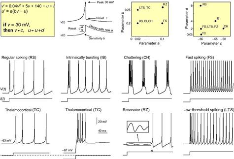
Figure 5.3 The Izhikevich simple model is a system of two linear differential equations that reflect the time derivatives (v′ and u′) of a fast membrane potential variable v and a slow ionic current variable u. The parameters a, b, c, and d can be measured in real neurons. The parameter I is the injected sum of synaptic input current amplitude. By varying the parameters in the model, the simple model can accurately describe the dynamic behavior of a very large number of neurons, some of which are shown here.14 (For color version of this figure, the reader is referred to the online version of this book.)
The v variable in Fig. 5.3 reflects the fast postsynaptic graded potentials that are evoked by the synaptic input current denoted by I; the u variable reflects a slower membrane current recovery variable that likely would be intrinsic to specific types of neurons and synapses and describes the recovery of membrane currents back to equilibrium. The v variable reflects inputs in the form of graded potentials that originally arise at synapses, whereas the u variable(s) is an intrinsic variable that is similar to what statistical modelers would call an intercept in that it controls the prior probability of a response although it exhibits slow time varying dynamics. The parameters, a, b, c, and d are the properties that can be measured in real neurons. Given these measured parameters, the dynamic firing properties are then entirely determined by the coefficient weights of the u and v variables in these equations.
The simple model in Fig. 5.3 is just an estimate of the simplest model needed to reproduce neural dynamics in a wide variety of neurons, but some real neurons could be adequately modeled with a zero weighting of the quadratic v2 term or linear v term. In fact, the simple model allows for a more general model that would allow for variation in the weighting of the v or v2 term, or for terms to be dropped.16 This simple model is apparently very sensitive to the choice of the after spike resetting cutoff parameter and can be unwieldy in hardware implementations for that reason. Alternative models that employ either a quartic v4 or an exponential term instead of v2 may not have this problem,17 although adjustments can be made to the parameters of the simple model to avoid such instability.18 In any case, models that have a quartic term in addition to a linear term rather than an exponential term exhibit sustained subthreshold oscillation, which is believed to a better model for the dynamics of some types of neurons.19 Thus, this characterization of neural dynamics continues to be an evolving field, but it does seem to be the case that one or more nonlinear terms, such as v2 or v4 may need to be used as potential basis features in these equations. It is also likely that real neurons are more complex than these simple possibilities, as a predominant v3 term also could be a more realistic possibility in at least some neurons in what is known as the Fitzhugh–Nagumo model.20 The reality is that all neurons are different,21 so such diversity would be very much expected across real neurons.
These models like the Izhikevich simple model are quite general and could reflect dynamics within dendrites, at the soma, and along the axon. The dendritic tree of a neuron often has extensive branching, so this allows for signals originating from diverse presynaptic inputs to interact at junctions in this branching. To simplify simulations, dendritic computations can be modeled as separate computations that employ this same simple model within each small dendritic compartment.22 These multicompartment models typically treat the change in graded potentials across time or v′ in this simple model as a sum of all graded potentials v in neighboring compartments.23 In this case, the equation that describes v′ in a given compartment then becomes a complex sum of similar expressions across all preceding compartments24 but with many different graded potential variables and can be represented by a multiple regression equation.25 So the v variable in this equation would be more realistically depicted as a vector with each element in the vector reflecting a feature given by a different presynaptic neuron, and with the coefficient weight also allowed to vary with each element and with associated nonlinear effects. Thus, this equation describing the change in soma graded potentials per unit change in time or v′ becomes a complex regression equation with many graded potential effects determining the probability of axonal spiking and this could be represented in a multiple logistic regression model.
An even more realistic model might allow for many independent interaction effects between separate presynaptic inputs, as this would be consistent with discussions about the nonlinear and coincident interaction computational properties of dendrites.26 A large number of main effect variables in the vector v and associated nonlinear effects such as v2, v3, or v4 along with a much larger number of associated interaction effects at junctions between dendritic branches are possible with many spatially diverse dendritic compartments. These many inputs and associated interaction and nonlinear effects that would arise are interpreted to be independent variables in the RELR statistical model. Thus, unlike classic neural network models which learn synaptic weights across synaptic inputs, RELR as a model of individual neural computation might be interpreted to be a model of the learning of the weights that arise in a complex dynamic model at the region of the soma that ultimately determines axonal spiking.
Technically, graded potential effects at the soma are not directly related to synaptic weights because they are determined by the passive cable and active dendritic spiking properties of the neuron that reflect interaction and nonlinear dynamic effects within neurons. However, in a neural computation model, RELR regression coefficient weights could still be viewed as memory weights that are indirectly affected by synaptic learning. Also, the RELR memory weights would directly impact the probability of neural spiking in such a model, but they just would not be synaptic weights. Understandably, multicompartment neural dynamic models wish to separate synaptic weights from neural dynamic effects.27 But this combination of all such weight effects into a potentially high-dimensional multiple logistic regression model that determines spiking probability at the soma has its advantages in that it becomes an aggregate representation that is tractable analytically as modeled in the RELR method, whereas more complex multicompartment models only can be understood through simulations. This also allows one to interpret the RELR computations in terms of putative learned computations performed within neurons that determine axonal binary spiking at the soma. Thus, RELR is clearly different from traditional neural network models that attempt to model synaptic weight learning directly,28,29 as RELR models the learning of weights that arise at the soma through a combination of neural dynamic and synaptic learning effects.
So, whereas the Izhikevich simple model and similar models are describing how neural dynamics are determined through realistic weight parameters, RELR as a neural model simply characterizes how the memory weights in these models would arise through learning, where learning is defined very broadly to mean genetic and environmental historical learning. Thus, the coefficients of the fast membrane potentials vector v and all associated nonlinear and interaction effects in neural dynamics models are the very same posterior weight parameters that the RELR method learns automatically through the maximum entropy subject to linear constraints method. Prior genetic or environmental weighting can be interpreted to be prior weights that can be unique to each feature (Appendix A4), which functions in a similar way to the u slow ionic current variable in the Izhikevich simple model in that it can be slowly varying in time until it abruptly is updated with binary spiking. RELR's learning results in optimal posterior coefficient memory weights that maximize entropy subject to all independent variable constraints. The independent variable features may be highly multicollinear features that include all main input effects and resultant interaction and nonlinear effects in what could be a massively high-dimensional statistical model as in Implicit RELR, or a parsimonious feature selection model that selects very specific main or interaction or nonlinear effects through Explicit RELR.30
3 Small Samples in Neural Learning
Through cached, online small sample update learning in working memory, the brain seems to be able to learn novel complex input patterns very quickly. Some medial temporal lobe neurons actually show single-trial learning in recognition memory tasks,31 although a single learning trial may be associated with numerous bursts of many binary responses in a single neuron, and rehearsal of the very same binary spiking input pattern presumably also may take place in working memory. Yet, the total number of binary responses still must be relatively very small for stable learning in a single neuron with a complex input pattern such as in recognition memory discrimination. In fact, humans can learn the meaning of a new word in the course of seconds.32,33 The maximal firing rate of neurons is expected to be roughly 1000 spikes/s, but the average firing is expected to be much lower. So, within hundreds of binary responses, typical neurons involved in higher level cognitive functions such as recognition memory or semantic memory may begin to show learning.
Just as is supposed to be happening in neural learning, RELR is a computational engine designed to learn the probability of binary outcomes given a small sample of training observations which also potentially has a very large number of independent features. Unlike standard predictive analytic methods, RELR estimates the probability of error and the probability of these binary outcomes. For this reason, RELR is able to remove error and produce solutions that are much more stable and much less prone to error with small observation samples and/or large numbers of multicollinear independent features.
Some process must be going on in neural learning that is quite different from standard regression methods because neurons must have an ability to learn with relatively small numbers of spiking responses compared to a huge number of inputs and associated nonlinear and interaction effects. For example, a typical neuron receives input from 10,000 neurons.34 Even if there is much overlap in these binary inputs such that they essentially code a smaller number of multicollinear continuously-valued features, there still would be a very large number of candidate features. With only 1000 independent input features from separate neurons, there would be the same number of 1000 independent linear input variables in a regression model that are likely to be highly multicollinear. With two-way interactions between linear variables, this would yield 501,000 total effects to consider including the interaction effects.35 If nonlinear effects up to a fourth-order polynomial are allowed, this would give over 2,000,000 largely multicollinear effects in a regression model.36 The traditional 10:1 rule of thumb that stated that one needs 10 response observations per linear variable does not apply here due to the nonlinear and interaction effects. So, a more general Dahlquist and Björk rule37 which requires a vastly greater number of observations is needed. This more general rule of thumb would require a million binary outcome observations with only 2000 independent variable effects and a thousand million such observations with only 60,000 variable effects that include nonlinear terms such as interaction effects. Even with only 501,000 independent variable effect terms as in this original example which only includes two way interaction effects, such processing would require >348,600 hours,38 which would be close to 40 years for a single neuron to learn the input response pattern.
So obviously neurons cannot learn in accordance with standard regression methods because those methods require such huge numbers of observations to avoid multicollinearity and overfitting error. There are some newer methods such as Random Forest, L2 regularization or Ridge Regression, L1 regularization or LASSO, and Support Vector Machines that deal with this error problem through averaging of different solutions or through regularization, which can work to smooth away at least some error. But these methods still have fairly unstable parameters and overfitting error with small samples, along with arbitrary parameters to control the degree of smoothing or averaging.39,40 There are also multilayer supervised neural network methods that incorporate similar regularization as Ridge Regression41 and also can show better prediction in small samples. But they also have similar problems as Ridge Regression with unstable parameters and overfitting in small samples, along with an arbitrary smoothing parameter that will change when a different arbitrary cross-validation procedure is used to tune this regularization parameter. Naïve Bayes is known to give relatively accurate prediction and stable parameters with very small training samples.42 But Naïve Bayes cannot see interactions and is susceptible to overfitting. In general, all the traditional methods seem to require too much training data to reflect the neural learning method or have other problems. Another possibility is that massively parallel groups of neurons could use many independent methods or modeling parameters and then average their results so that error in small sample learning is averaged out. This would work if the massively parallel learning used a significant number of independent methods that give reasonable importance sampling as can be done in effective stacked ensemble model learning. However, it is hard to understand how the brain evolved or learned such a complex process as stacked ensemble learning. As reviewed in the initial chapter, even though implicit memory models do seem similar to ensemble models once they are learned, these stacked ensemble models do not allow the automatic learning that would be expected in the brain's implicit learning.
A much simpler explanation would be that the basic neural calculus has evolved to learn most probable responses that are very effective at removing error probabilities. A common theme in all previous attempts to handle error in predictive analytic methods is that error is not viewed from the perspective of a probability model. As reviewed in the initial chapter, various regularization methods like LASSO and Ridge do not estimate the error in terms of probability of error that sum to one for each independent variable, as the L1 and L2 penalty terms are not probability measures but are instead arbitrarily weighted nonprobability functions. By contrast, RELR estimates the probability of all outcome and error events given the input features. Because of this accurate error probability modeling, RELR automatically handles error and produces small sample learning with high-dimensional multicollinear inputs.
As a neural model, the RELR error model is assumed to be the natural outcome of a maximum entropy process where graded potential effects sum at the soma so that the probability of positive and negative errors cancel. The Hebbian learning principle is one of the most widely applied ideas in neural learning; it is that “neurons that fire together wire together”.43 In a broader sense where both positive and negative correlation drives learning, spike-timing effects in this RELR process could determine that input effects that are poorly correlated with the spiking output of a neuron would not influence the learning mechanism just as RELR's feature reduction removes small magnitude effects. Moreover, RELR's implicit and explicit selection methods have a strong preference for feature effects that are more positively or negatively correlated with binary output spiking patterns just as would occur with spike-timing dependent learning. Unlike stacked ensemble learning, the Explicit and Implicit RELR maximum probability methods could be embodied in individual neurons. Unlike all these other methods that require extra model tuning based upon arbitrary cross-validation samples to avoid overfitting, RELR's learning mechanisms are completely automated and entirely based upon the training sample. In addition, RELR's sequential Bayesian online learning method could directly occur in sequential phases of cached, small sample “working memory” update episodes. Taken as a whole, these computational properties of RELR are the characteristics that might be expected in real neurons in the brain that are the basis of learning and memory.
4 What about Artificial Neural Networks?
These suggestions that RELR could be a reasonable model for the calculus that determines learning and memory in real neurons may cause some to remember the claims made by artificial neural network modelers in the early 1980s. I recall being at a packed conference at UC-Irvine in the mid-1980s when there was great excitement about the newer artificial neural networks. The single-layer perceptron proposed in the 1950s had been the original neural network method.44 As Marvin Minsky famously showed, this single-layer perceptron could not learn Exclusive OR and Exclusive XOR predictive relationships, which are what statisticians would call interactions.45 So the single-layer perceptron had classifier properties that are about the same as would be expected from a standard logistic regression model without interactions. Much of the excitement in the 1980s concerned the fact that new multinode and multilayer artificial neural networks finally could model interactions effects.46 In fact, there was unbelievable optimism back then that these new artificial neural networks were reflections of the brain's cognitive computation mechanisms. Yet, very few of the promises from the great hype of the 1980s have been realized.
The neural networks that grew out of the 1980s were actually a large number of different methods but one of the most popular methods was a supervised neural network that most often employs the back-propagation method across a multilayer network of artificial neurons that includes a hidden layer. These multilayer perceptrons are designed to minimize the difference between the target or supervising signal and the output of the system. Because of the hidden layer, these multilayer perceptrons suffer because they are black boxes which are not transparent in terms of understanding how they work. Another problem is that there has never been general empirical support for supervised back-propagation learning across a network of neurons in the brain. However, there is now some evidence that a back-propagation learning mechanism could exist within individual neurons. This within-neuron back-propagation mechanism is thought to be involved in spike-timing-dependent learning processes.47 There has been a fairly recent proposal that a multilayer perceptron using the 1980s back-propagation idea could involve a dendritic hidden layer within neurons and explain neural learning computations.48 Yet, a number of questions have been raised as to whether this model's dendritic hidden layer computations could actually happen in real neurons.49 Even if the new knowledge about within-neuron learning mechanisms could be aligned with these classic supervised artificial neural network methods, these multilayer back-propagation methods from the 1980s have a more fundamental flaw that was reviewed in the last section. Even when they employ regularization to attempt to smooth away error, parameters are still too unstable and tend to overfit too much in small sample sizes and with large numbers of multicollinear features to be a reasonable model for neural learning.
Another well-known method from the 1980s was the Hopfield neural network depicted in Figure 5.4.51 In a fully connected Hopfield neural network, each node is considered to be a neuron which is connected as an input to all other neurons and which receives all of its inputs from all other neurons. The Hopfield neural network is a recursive network that requires feedback in order to compute its weights in a model of associative memory in that each input learns to be associated with all others in network. Hopfield networks suffer from the problem that its solutions are not ensured to be globally optimal, and instead are often local minima. Hopfield networks are closely related to Boltzmann machines which are another type neural network method with roots in the 1980s. The major difference is that the Boltzmann machine's optimization is stochastic and can use simulated annealing which might help it escape local minima,52 whereas the Hopfield network employs a deterministic method.53
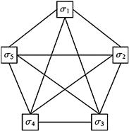
Figure 5.4 A schematic of a fully connected Hopfield neural network.50
The original Boltzmann machine suffered from difficulties in converging in reasonable periods of time with more complex problems, but Restricted Boltzmann machines are now used which simplify the connection architecture in the original Boltzmann machine to produce much faster computation although hidden units are still usually employed, and back propagation may be used in deep learning tasks.54 New formulations also have been proposed to help with some of the more severe problems in Hopfield networks.55 Yet, this can change the basic simple functionality and interpretation by imposing learning mechanisms that are no longer based upon simple cross-products to increase network capacity.56
RELR is similar to Restricted Boltzmann machines, Hopfield networks, and even the multilayer back-propagation perceptron in the superficial sense that it is also an optimization method. But RELR also takes into account errors-in-variables. For this reason, RELR may be more likely to find estimates of global maxima that generalize well to new observation samples. In this sense, RELR's error modeling also may be similar to what occurs in real neurons in that it allows very high-dimensional modeling in small samples that avoid unstable solutions and overfitting. Another advantage is that RELR allows online sequential learning, along with causal learning, in completely automated machine learning computations that are at least putatively similar to neural computations in ways that ultimately could be tested empirically.
Other artificial neural network methods developed in the 1980s were unsupervised neural networks, which can be used in dimension reduction tasks. Neural networks designed to categorize visual images like dogs and cats into groups of objects often have an early unsupervised processing stage that may be almost equivalent to K-mean clustering, as exemplified in the work of Riesenhuber and Poggio.57 This dimension reduction stage reduces extremely high-dimensional input data into a manageable smaller set of input features for later supervised neural network processing.58 Another well-known unsupervised neural network approach from the 1980s is the Self-Organizing Map method which is essentially a form of nonlinear Principal Component Analysis.59
A problem with the supervised and unsupervised neural network dichotomy from the 1980s is the nagging question about whether the brain actually performs supervised versus unsupervised learning. In fact, one very influential view in today's neuroscience is that the classic supervised versus unsupervised neural learning dichotomy from the 1980s is very artificial and is not the way that the brain actually works.60 This argument is that the relationship between neurons and their input effects should be interactive rather than supervised or unsupervised and thus may depend upon resonance between binary neural spiking and local field potentials. In accord with this alternative view, one artificial neural learning method that was first introduced in the 1980s is fundamentally different from methods that assume that the brain must have separate supervised and unsupervised learning mechanisms. This is the neural Darwinism approach popularized by Nobel Laureate Gerald Edelman and other prominent scientists.61–63
Neural Darwinism assumes that neurons learn by selecting input patterns of activity, or neuronal groups. This is assumed to occur as neural spiking output patterns resonate with input effects in a natural selection mechanism that is akin to the mechanism at work in the evolution of species. With this emphasis on spike-timing-dependent plasticity as a fundamental neural learning mechanism and given the evidence for spike-timing plasticity mechanisms reviewed in the next chapter, neural Darwinism and this theory of neuronal group selection may be closer to how neurons actually work than all the other neural network methods from the 1980s.64 Neural Darwinism is similar to genetic programming in that it is inspired by genetic principles of natural selection, but it also differs from genetic programming in respect to replication in that it is much more of a random search. For reasons connected to this random search, neural Darwinism is not without critics,65 especially in reference to a poor ability to produce neural learning that is capable of self-replication. Replication is one of the hallmark genetic actions as observed in DNA mechanisms, but it is argued that neural Darwin mechanisms would produce too many false positive and negative errors to allow neural learning patterns to self-reproduce.66 While other evolution inspired methods like genetic programming can lead to replication, they also require arbitrary user-dependent parameters that determine mutation and cross-over. For this reason, genetic programming models can have the same flaws related to arbitrary user parameters as the other standard predictive analytic methods.
Neural Darwinism has had success in the neuroscience community as evidenced by its influence in ongoing projects to simulate learning in large networks of artificial neurons.67,68 Therefore any improved method designed to model neural computation likely will need to consider those aspects of neural Darwinism that have been most effective. Like neural Darwinism, RELR's implicit and explicit learning methods are also each not just passive but rather interactive as the ultimate mechanism of these RELR methods is to select optimal and most probable weights based upon how input effects resonate with spiking outputs. Like neural Darwinism, RELR avoids the artificial dichotomy between supervised and unsupervised neural learning. Therefore, unlike supervised neural networks that require separate unsupervised neural networks to perform dimension reduction preprocessing, RELR can model dimension reduction built into individual neurons based upon magnitude of correlations between input effects and spiking output. In this way, RELR could be a model for the brain's neural computation through resonance between local field potential input effects and binary spiking without a need for separate unsupervised networks to perform dimension reduction preprocessing.
Unlike neural Darwinism, RELR allows interpretable and understandable solutions in terms of parsimonious feature selections that are stable and do not depend upon a random search that causes variability in selected features across independent representative training samples. This stability in RELR's learning is due to accurate error modeling which allows most probable features easily to be discovered. RELR is also able to produce output patterns that perfectly replicate input patterns, so under balanced sample zero-intercept conditions it will avoid the quasi-complete separation convergence problems that plague standard logistic regression, and RELR never will show complete separation problems due to its error modeling. However, RELR is not designed to model genetic mechanisms but is instead designed to model neural computations so any analogy to evolutionary and genetic mechanisms might ultimately break down.
RELR's advantage over a random search is not just in stability and error avoidance. This is because RELR's gradient ascent directly optimizes and is thus substantially faster than the slow, random neural Darwin search. In fact, RELR yields identical solutions as the maximum entropy subject to linear constraints method and has a physical and neurophysiological interpretation. That is, RELR's fundamental maximum entropy-based learning mechanism can be considered to reflect a basic physical mechanism that necessarily must be embodied in neurons. The tendency to find physical solutions that maximize entropy subject to all other available constraints is assumed to be a basic physical law, the Second Law of Thermodynamics. So the RELR learning mechanisms in real neurons would be expected to obey the same basic physical maximum entropy mechanism that has constrained neural dynamics from Hodgkin and Huxley onward.69
To the extent that it might have any similarity to neural computation, RELR should not be thought of as a neural network computation model reflecting specific connections between individual neurons. Instead, any modeled neural computation might be thought to represent the modal activity of an ensemble of similar neurons where the variability in posterior memory weights is given by the standard error of RELR's posterior regression parameters. In fact, a RELR neural ensemble may be itself built from inputs that are also ensembles of neurons. In this neural ensemble, each input and output should be viewed as a collection of neurons which can take on a more continuous range of outputs than binary signals, so the probability of a RELR binary output response given the input features would be a better description of the ensemble output than the actual predicted binary output response. This probabilistic description accords with the idea that RELR as a neural computation model is consistent with local field properties of a neural ensemble, as local field potentials are closely correlated with the time histogram that describes the probability of spiking responses in local neural populations.70 Although RELR does incorporate typical network concepts of feed forward and feedback signals in its implicit and explicit processes, these concepts also could be associated with field properties of aggregate population signals in the brain which as Nunez and collaborators show are believed to have both traveling and standing wave-like properties.71 Thus, traveling waves may move only in one direction and be feed forward signals, whereas standing waves arise from traveling waves that feedback to an original source and continually resonate. This resonant feedback results in highly structured periodic disturbances like vibrations in a violin string, and Nunez argues that similar standing waves could be the basis of highly structured momentary oscillating neural ensemble synchrony.
As a model of neural computation, probably the most serious problem with supervised neural networks is that they are supervised. This creates a need for a ghost in the brain to supervise these networks with training labels. RELR can be viewed as a supervised method because it does require training labels which are the spiking binary responses in postsynaptic neurons. Yet, as with neural Darwinism methods, these binary spiking events also could be viewed as arising from an interaction between input feature signals and local field potentials that is guided by natural neural selection mechanisms at work in both implicit and explicit processing. Through this selection, explicit or implicit neural computation could result from the interaction between binary spiking events and the brain's local field potentials with the direction of causality being in either direction, so spikes that are driven by input features may lead to local field reflections of postsynaptic potentials in adjacent neurons or local field potentials may influence binary spiking. In fact, there is new evidence that binary spiking responses in a local neural population can be caused by spatiotemporal patterns in local field potentials.72 Thus, in RELR's information theory of neural computation, there is no need for a supervising ghost in the brain as both unconscious and conscious cognitive functions may arise through stable interactions between local field potentials and spiking neurons.
Back in the 1980s, nobody had considered that standard supervised multilayer neural networks would have significant overfitting and multicollinearity error problems with high-dimensional data. Back then, there was less concern about the general lack of insight into how these artificial neural network learning mechanisms could be embodied in real neurons. Back in the 1980s, nobody yet thought that extensive dendritic arborization could produce interaction effects within neurons without recourse to multiple layers of processing across neurons. Back then, there was very primitive understanding of spike-timing-dependent plasticity processes involving long-term potentiation and depression, so the idea that resonance is basic to neural learning was not that popular. Back then, all neural-inspired models were implicit learning models that only produced hidden units and black box solutions, as there was not yet a full realization that explicit learning was a fundamentally different process.
The past 30 years have produced enormous advances in neuroscience and the pace of advance seems to be quickening. One area that has produced especially important progress concerns how mechanisms of cognition, learning, and memory may be related to synchronous oscillations in resonating groups of neurons in accord with spike-timing plasticity mechanisms. Yet, these principles really have not yet made their way in any impactful sense into machine learning theory and application. The next chapter gives an overview of oscillating synchrony as a fundamental organizing principle of cognitive neural computation.