
4.6. Empirical illustrations: linear mixed models with REML
In this illustrative section, the main objective is to examine whether the ML and REML estimators in linear mixed models yield different values of parameter estimates and approximates. The method for approximating the random effects for each subject is also displayed. Based on the prediction of the random effects, the model-based trajectories of the response variable are then displayed, both individually and group-averaged. The two datasets described in Chapter 3 continue to be used for illustrations: one concerning the effectiveness of acupuncture treatment on PTSD symptom severity and one analyzing the effect of marital status on an older person’s disability severity score.
4.6.1. Linear mixed model on effectiveness of acupuncture treatment on PCL score
The primary objectives in the first illustration are to compare the results from the ML and the REML estimators and to predict subject-specific random effects in linear mixed models, using longitudinal data of a small sample size. Therefore, data of the DHCC Acupuncture Treatment study continues to be used. The model specification and the covariate definitions remain the same as those in Chapter 3. Specifically, the time factor, named TIME, is a continuous variable with 0 = baseline survey, 1 = 4-week follow-up, 2 = 8-week follow-up, and 3 = 12-week follow-up. The treatment factor, TREAT, remains the same dichotomous variable with 1 = receiving acupuncture treatment and 0 = else. The time factor is partitioned into the linear, quadratic, and cubit components, all centered to reflect a curvilinear pattern of change over time in the dependent variable PCL_SUM.
Given the use of the same linear mixed model, SAS Program 3.1 can be used with minor modifications, as presented below.
SAS Program 4.1:

Compared to SAS Program 3.1, there are several distinct modifications in SAS Program 4.1. First, the METHOD = option is modified from METHOD = ML to METHOD = REML in the PROC MIXED statement. Given its popularity in the application of linear mixed models, the REML is the default in SAS for the METHOD = option, and therefore, without specifying this option, SAS produces the same analytic results. Second, the COVTEST option is added, requesting SAS to display asymptotic standard errors and Wald tests for covariance parameters. Third, this program adds the option SOLUTION in the RANDOM statement, informing SAS to produce the empirical BLUPs of the random effect parameters and the corresponding standard errors for each subject by applying shrinkage. Given these additional options, the BLUP predictions of PCL_SUM are saved into the temporary data file PRED for generating the trajectory of individuals. Lastly, the PROC SGPLOT procedure is applied to generate two sets of intraindividual growth curves: one for those receiving acupuncture treatment and one for those in the control group.
For the convenience of comparing the fixed-effect estimates and the model fit statistic between the ML and REML estimators, relevant results derived from SAS Programs 3.1 and 4.1 are summarized in Table 4.1.
Table 4.1
Regression Coefficients and Model Fit Statistic on PCL_SUM From ML and REML Estimators: DHCC Acupuncture Treatment Study (N = 55)
| Explanatory Variable | Parameter Estimate | Standard Error | Degree of Freedom | t-Value | p-Value |
| Estimates of Fixed Effects From MLE | |||||
| Intercept | 51.99** | 2.47 | 50.20 | 21.06 | <0.01 |
| CT | 1.24 | 2.30 | 56.30 | 0.54 | 0.59 |
| CT_2 | −0.51 | 0.72 | 49.80 | −0.70 | 0.49 |
| CT_3 | −1.91* | 1.06 | 46.20 | −1.80 | 0.08 |
| TREAT | −13.44** | 3.60 | 53.00 | −3.74 | <0.01 |
| CT × TREAT | −0.40 | 3.46 | 57.80 | −0.11 | 0.91 |
| CT_2 × TREAT | 5.30** | 1.07 | 50.8 | 4.97 | <0.01 |
| CT_3 × TREAT | −1.07 | 1.58 | 47.00 | −0.68 | 0.50 |
| −2 log-likelihood | 1399.60 | ||||
| Estimates of Fixed Effects From REML | |||||
| Intercept | 51.99** | 2.52 | 48.30 | 20.64 | <0.01 |
| CT | 1.24 | 2.35 | 53.90 | 0.53 | 0.60 |
| CT_2 | −0.51 | 0.74 | 47.80 | −0.69 | 0.50 |
| CT_3 | −1.91* | 1.08 | 44.20 | −1.77 | 0.08 |
| TREAT | −13.44** | 3.67 | 51.00 | −3.66 | <0.01 |
| CT × TREAT | −0.40 | 3.55 | 55.30 | −0.11 | 0.91 |
| CT_2 × TREAT | 5.30** | 1.09 | 48.70 | 4.86 | <0.01 |
| CT_3 × TREAT | −1.07 | 1.62 | 45.00 | −0.66 | 0.51 |
| −2 log-likelihood | 1,383.50 | ||||

Notes: CT, centered time; CT_2, quadratic centered time; CT_3, cubit centered time.
* 0.05 < p < 0.10.
** p < 0.01.
Table 4.1 displays that the point estimates of the fixed effects from the two estimators are all identical. Additionally, the standard error estimates from the REML estimator are all greater than those from MLE, but the degrees of freedom for REML are all slightly lower than those from MLE. As a result, the t scores and the resulting p-values are very close between the two sets of results. The values of the likelihood ratio statistic obtained from the two estimators are also similar, thereby leading to the same conclusion concerning the model fit. Therefore, even with a small sample size, the ML and the REML estimators produce very close parameter estimates and the model fit statistic.
The results for the Type 3 tests of the fixed effects from MLE and the REML estimators are also similar, summarized in Table 4.2.
Table 4.2
Type 3 Test Results of the Fixed Effects on PCL_SUM From ML and REML Estimators: DHCC Acupuncture Treatment Study (N = 55)
| Explanatory Variable | Numerator DF | Denominator DF | F-Value | p-Value |
| Test Results From MLE | ||||
| CT | 1 | 57.80 | 0.36 | 0.55 |
| CT_2 | 1 | 50.80 | 16.18 | <0.01 |
| CT_3 | 1 | 47.00 | 9.61 | <0.01 |
| TREAT | 1 | 53.00 | 13.96 | <0.01 |
| CT × TREAT | 1 | 57.80 | 0.01 | 0.91 |
| CT_2 × TREAT | 1 | 50.80 | 24.72 | <0.01 |
| CT_3 × TREAT | 1 | 47.00 | 0.46 | 0.50 |
| Test Results From REML | ||||
| CT | 1 | 55.30 | 0.34 | 0.56 |
| CT_2 | 1 | 48.7 | 15.46 | <0.01 |
| CT_3 | 1 | 45.00 | 9.18 | <0.01 |
| TREAT | 1 | 51.00 | 13.40 | <0.01 |
| CT × TREAT | 1 | 55.30 | 0.01 | 0.91 |
| CT_2 × TREAT | 1 | 48.70 | 23.63 | <0.01 |
| CT_3 × TREAT | 1 | 45.00 | 0.44 | 0.51 |

Notes: *0.05 < p < 0.10; **0.01 < p < 0.05; ***p < 0.01.
The two sets of the Type 3 test results are strikingly similar, particularly the p-values. Combining the comparative results displayed in Tables 4.1 and 4.2, it is evident that the ML and REML estimators produce very close fixed-effect estimates, both point and standard error, and also, the model fit statistics.
Given the addition of the COVTEST option in the PROC MIXED statement, the asymptotic standard errors and the Wald tests for covariance parameters are obtained, as presented in the following output table.
SAS Program Output 4.1a:

Given the above Covariance Parameter Estimates table, the variance of within-subject random errors is estimated as  , statistically significant. An unstructured (3 × 3) variance–covariance matrix G for the three random effect components can be created from the table, given by

As defined, the diagonal elements in the G matrix are the variance estimates of the random effects for the intercept (134.97), the linear time component (5.28), and the quadratic polynomial term of centered time (0.59), respectively. The off-diagonal elements display the covariance of each pair of the random effects. The subject-specific random effects for the intercept are positively associated with the random effects for the linear time polynomial (cov = 21.14) and negatively related with the random effects for the quadratic term (cov = −4.28). The random effect covariance between the linear and the quadratic time polynomials is −2.46. With α = 0.05, only the variance estimate of the random intercept and the covariance between the random intercept and the random slope for the linear time term are statistically significant. This type of test, however, is only asymptotically valid, and therefore, the test results are trustworthy just for large samples.
The above Covariance Parameter Estimates table displays the variance–covariance parameter estimates specified in the G and R matrices, and therefore, they are not the estimates for the empirical BLUPs. The empirical BLUPs for the random effects and their standard errors are derived from the SOLUTION option in the RANDOM statement. The following output table presents the random effect approximates for the first five subjects in the data.
SAS Program output 4.1b:

It may be emphasized that  is a shrinkage predictor, so that
  (McCulloch and Neuhaus, 2011). Although the empirical BLUPs are heavily influenced by the normality hypothesis for the random effects, the distribution of
  does not accurately represent the distribution of the random effects due to shrinkage toward the population mean. This property can be empirically effective to correct for misspecification of assumed distributions of the random effects. These issues will be further discussed in Chapter 7.
Given the fixed-effect estimates and the subject-specific random effect approximates, the SGPLOT procedure generates two model-based time plots of trends in the PCL score, with the first plot for those receiving acupuncture treatment and the second for those in the control group.
Figure 4.1a and b displays that compared to the descriptive time plots presented in Chapter 2 (Fig. 2.1a and b), the model-based trajectories in PCL_SUM appear smoother. Generally, those receiving acupuncture treatment display sharper declines over time in the PCL score than those in the control group, particularly at early times. However, the trajectory of individuals does not apparently manifest the effectiveness of acupuncture treatment on the PCL score. It may be useful to plot the population-averaged time trend for generating a pattern of change over time and its differences between the two groups. The following SAS program is created to generate the population-averaged PCL scores for the two treatment groups.


Figure 4.1 (a) Subject-specific time plots on PCL score for treatment group: mixed model. (b) Subject-specific time plots on PCL score for control group: mixed model.
SAS Program 4.2:

In SAS Program 4.2, the PROC SQL procedure creates a temporary SAS data file NEW from the dataset PRED. Next, the predicted mean PCL_SUM score, named PCL_PRED, is computed for each treatment group and at each time point by using the GROUP BY TIME, TREAT clause. The mean PCL_SUM scores are then saved into the temporary data file NEW. In the PROC SGPLOT procedure, the option GROUP = ID in SAS Program 4.1 is replaced with GROUP = TREAT that asks SAS to generate a plot for each treatment group instead of for each subject. Figure 4.2 displays the plot.
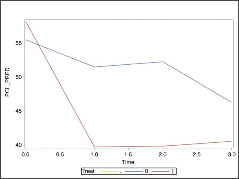
Figure 4.2 Time Plots of Predicted PCL Score for Treatment and Control Groups: Mixed Model
Figure 4.2 plots the time trends in the mean PCL score for the two treatment groups. The two predicted curves across the four time points take tremendous resemblance to the descriptive pattern (Fig. 2.2), reflecting a strong impact of acupuncture treatment on PTSD symptom severity. During the first month after treatment, patients receiving acupuncture treatment are expected to experience a much sharper decline in PCL_PRED than those in the control group. After the second time point, this reduced predicted mean score stabilizes throughout the rest of the observation period.
4.6.2. Linear mixed model on marital status and disability among older Americans
In the second example, I continue to use the longitudinal data from the AHEAD survey for the application of the REML estimator in the linear mixed model. As described in Chapter 3, data of six waves are used, starting with the 1998 wave (1998, 2000, 2002, 2004, 2006, and 2008). This analysis is focused on the effect of an older person’s marital status on disability severity in older Americans and its pattern of change over time. The dependent variable remains the health-related difficulty in performing five activities of daily living (dress, bath/shower, eat, walk across time, get in/out of bed), measured at six time points and named ADL_COUNT. The value of ADL_COUNT ranges from 0 to 5 at each time point. Given the results of a preliminary data analysis, only the linear term of time is specified in the linear mixed model. Marital status, named married in the analysis and time-varying, is the same dichotomous variable with 1 = currently married and 0 = else. The control variables still include the three centered covariates: Age_mean, Educ_mean, and Female_mean. Given the same set of covariates, the linear mixed model specified in Section 3.5.2 is used, with the exception of applying the REML estimator to find the parameter estimates. In the analysis, I compare the differences in the parameter estimates from the ML and REML estimators, respectively. The random effects are approximated by using the BLUP approach. Additionally, two model-based trajectories of the mean ADL count are generated: one for those currently married and one for those currently not married.
In generating the two growth curves, a technical problem arises. While some control variables are considered in the mixed model, each subject has a predicted value of ADL_COUNT at each of the six time points given one’s covariates’ values and the unique random effect approximates. If the two time plots are directly displayed from the predicted ADL count, the pattern of change over time in the ADL prediction and its group differences may be confounded by the effects of age, education, or gender. To generate nonconfounded effects of marital status, two hypothetical population groups need to be compared, who differ only in marital status while all the control variables have the same values.
There are two statistical approaches for handling this problem. One approach is to generate model-based linear predictions by computing the least squares means while holding controls at sample means. The other method is to create a scoring dataset for constructing two hypothetical population groups. The least squares mean approach computes the predicted marginal means with the fixed effects, assuming a balanced population. In this analysis, I apply the second approach first, given the focus of the chapter on the prediction of the random effects. Correspondingly, a scoring dataset is created in which the ADL count is specified as missing and the three centered control variables as zero (sample means) while the time factor and the marital status variable are retained. This scoring dataset is then combined with the observed data. The popular least squares means will be described in the next chapter.
The rationale for combining the observed and the scoring datasets is well established. As the ADL count is specified as missing, the hypothetical data are not included in the estimation of parameters, so that the inclusion of the scoring dataset does not have any impact on the quality of estimation and approximation. After the parameters are estimated or approximated, each observation has a predicted value of the ADL count given the covariates’ values, the estimated regression coefficients, and the predicted subject-specific random effects. Consequently, two sets of longitudinal trajectories of the predicted ADL count can be plotted: one for the actual population and one for the hypothetical population. In SAS programming, the generation of the two time plots can be accomplished by using the WHERE = statement in applying the PROC MIXED procedure. Below is the SAS program for creating the scoring dataset and the modified linear mixed model with the REML estimator.
SAS Program 4.3a:

SAS Program 4.3a first creates a scoring dataset by keeping the variables ID, TIME, and MARRIED from the original dataset and then specifying ADL_COUNT =. and each of the three centered controls equals 0. The DATA TP3 step combines the observed and the scoring dataset into one. The model part is similar to SAS Program 3.2 except for the use of the METHOD = REML option and the addition of several other options such as COVTEST in the PROC MIXED statement and SOLUTION in the RANDOM statement. The predictions of the ADL count are saved into the temporary data file PRED for creating growth curves, in the same fashion as applied in the first example.
Program 4.3a derives a set of REML estimates and approximates. In Table 4.3, I present the fixed-effect estimates and the model fit statistics from the ML and REML estimators, respectively.
Table 4.3
Regression Coefficients and Model Fit Statistic on ADL Count From ML and REML Estimators: AHEAD (N = 2,000)
| Explanatory Variable | Parameter Estimate | Standard Error | Degree of Freedom | t-Value | p-Value |
| Estimates of Fixed Effects From MLE | |||||
| Intercept | 1.33*** | 0.04 | 1726.00 | 32.53 | <0.01 |
| CT | 0.13*** | 0.01 | 4822.00 | 17.67 | <0.01 |
| MARRIED | −0.21*** | 0.05 | 300.00 | −4.08 | <0.01 |
| CT × MARRIED | −0.04*** | 0.01 | 4822.00 | −3.71 | <0.01 |
| Age_mean | 0.06*** | 0.00 | 1726.00 | 13.33 | <0.01 |
| Educ_mean | −0.06*** | 0.01 | 1726.00 | −6.81 | <0.01 |
| Female_mean | 0.29*** | 0.06 | 1726.00 | 4.63 | <0.01 |
| −2 log-likelihood | 19,897.3 | ||||
| Estimates of Fixed Effects From REML | |||||
| Intercept | 1.33*** | 0.04 | 1726.00 | 32.50 | <0.01 |
| CT | 0.13*** | 0.01 | 4822.00 | 17.66 | <0.01 |
| MARRIED | −0.21*** | 0.05 | 300.00 | −4.08 | <0.01 |
| CT × MARRIED | −0.04*** | 0.01 | 4822.00 | −3.71 | <0.01 |
| Age_mean | 0.06*** | 0.00 | 1726.00 | 13.31 | <0.01 |
| Educ_mean | −0.06*** | 0.01 | 1726.00 | −6.80 | <0.01 |
| Female_mean | 0.29*** | 0.06 | 1726.00 | 4.62 | <0.01 |
| −2 log-likelihood | 19,942.9 | ||||

*** p < 0.01.
Table 4.3 displays two sets of the fixed-effect estimates and the likelihood ratio statistics from MLE and the REML estimator, respectively. Except for a few trivial differences in the t scores, the fixed-effect estimates from the two estimators, consisting of point, standard error, degree of freedom, t statistic, and p-value, are all exactly the same. The values of the −2 log-likelihood are also very close, although they are derived from different types of data (the complete and error contrasts). The two estimators also yield very close Type 3 test results, not presented due to identical p-values. These identical or very close estimates provide very strong evidence that for large samples, the downward bias in MLE is negligible and therefore can be overlooked. In longitudinal data analysis, the researcher can choose either MLE or the REML estimator according to his or her needs as long as the sample size is sufficiently large.
SAS Program 4.3a, given the specification of the COVTEST option, also yields the estimates, the asymptotic standard errors, and the Wald tests for covariance parameters, as presented below.
SAS Program Output 4.2:

Given the above table, the variance estimate of within-subject random errors  is 0.56 (p < 0.0001). All covariance parameter estimates for the random effects are statistically significant, with p-values being smaller than 0.0001. An unstructured (2 × 2) variance–covariance matrix of the random effects for the intercept and the slope of time is created as follows:

The variance estimates of the random effects for the intercept and the slope of time are 1.727 and 0.033, respectively. Covariance of the two random effects is 0.135, displaying a positive but weak association. These test results are asymptotically valid given the large sample size used for this analysis. SAS Program 4.3a and b also produces the empirical BLUPs of the subject-specific random effects and their standard errors.
As indicated earlier, SAS Program 4.3a creates a combined longitudinal dataset, including twelve observations for each subject, with the first six being observed and the next six being hypothetical. As a result, both the actual and hypothetical trajectories of the ADL score can be plotted. Below is the SAS program for yielding the population-averaged growth curves.
SAS Program 4.3b:

In SAS Program 4.3b, the temporary dataset PRED is sorted first by time, and the mean of the predicted ADL count is then created for each marital status group and at each time point by the PROC SQL procedure. Two sets of longitudinal trajectories of the ADL count are constructed by the PROC SGPLOT procedure, with each set consisting of two trajectory curves: one for those currently married and one for those currently not married. In the first PROC SGPLOT procedure, the WHERE AGE_MEAN NE 0 AND EDUC_MEAN NE 0 AND FEMALE_MEAN NE 0 statement specifies two ADL growth curves for the actual population. Likewise, the second procedure creates the ADL trajectories for the hypothetical population by using the WHERE ADL_COUNT =. AND AGE_MEAN = 0 AND EDUC_MEAN = 0 AND FEMALE_MEAN = 0 statement. In this analysis, specifying FEMALE_MEAN NE 0 or FEMALE_MEAN = 0 only in the WHERE statement is sufficient to distinguish between the actual and the hypothetical populations because in real life, gender must be scaled either as 0 or as 1. Figures 4.3 and 4.4 display the resulting plots.

Figure 4.3 Time Plots of Predicted ADL Counts for Currently Married and Currently Not Married: Linear Mixed Model

Figure 4.4 Time Plots of Adjusted ADL Predictions for Currently Married and Currently Not Married: Linear Mixed Model
Figure 4.3 plots the evolution of two sets of ADL growth curves for the two marital status groups. For both population groups, the ADL count increases over time initially, and it then decreases consistently. The plot displays a distinctive separation between the two curves throughout the entire period of time, thereby reflecting the strong effect of current marriage on reduction in the disability severity. Figure 4.4, created by adjusting for the confounding effects of the control variables, verifies this pattern of change over time in the ADL count and its group differences. As the two figures are strikingly similar, the effect of current marriage on the time trend of disability severity in older Americans is not confounded by the theoretically relevant lurking variables. Considering the statistical significance of the fixed effect of marital status and the interaction with time, it can be safely concluded that the impact an older person’s current marriage has on disability severity is both statistically meaningful and substantively important after adjusting for confounding effects.
4.7. Summary
In longitudinal data analysis, one of the most remarkable progresses in the past three decades is the widespread application of the Bayes-type techniques. Bayes’ theorem and Bayesian inference provide a strong theoretical foundation for approximating unobservable parameters in mixed-effects models. The REML approach, which corrects the downward bias in the ML variance estimates, is an empirical Bayes method that models the marginal posterior predictive density for the variance components while formally integrating out the regression coefficient vector, β. Therefore, in this chapter I first described the basic specifications of Bayesian inference prior to the introduction of the REML estimator. The REML method is arguably a more reliable estimator to find parameter estimates in linear mixed models; nevertheless, for large samples the ML and REML estimators usually yield very close or even identical parameter estimates and approximates, as empirically evidenced in the Section 4.6.
In this chapter, the statistical techniques for predicting the random effects were delineated and discussed. In longitudinal data analysis, linear predictions are often required to generate the trajectory of individuals in the continuous response variable. Population-averaged growth curves can also be predicted from averaging over the random effects. In linear predictions, the BLUP and the shrinkage approach are regularly applied to approximate the random effects and predict the outcomes for each subject. In Section 4.6, a technique was delineated to adjust for potential confounding effects when creating population-averaged trajectories. In particular, a scoring dataset was constructed by retaining the variables of interest and creating some others for representing a hypothetical population.
Given the iid assumption for random errors in linear mixed models, linear predictions with adjustments for the confounding effects can also be conducted by using the least squares means, as will be described and illustrated in the next chapter. Briefly, least squares means are obtained by using the estimated regression coefficients, the selected covariates’ values, and the averages over the distribution of the random effects. While the scoring data approach directly computes the mean of BLUPs with shrinkage, the model-based approach in least squares means assumes longitudinal data to be balanced, and thus can generate different predictions for population groups. The two approaches, however, are expected to yield exactly the same predicted values of the response for the entire population given the condition that  . At the same time, as the
  is shrunk toward the population average
  ,
,  , and therefore, the least squares means are associated with greater standard error estimates than the scoring data approach. These issues will be further discussed in Chapter 7.
..................Content has been hidden....................
You can't read the all page of ebook, please click here login for view all page.