In regression modeling on longitudinal data, dependence of repeated measurements for the same subject needs to be taken into account. By specification of the random effects in the regression, a statistical model with mixed effects provides an efficient approach to handling intraindividual correlation. Some statisticians have attempted to analyze correlated data from a different direction, developing a simplified statistical approach referred to as generalized estimating equations, or GEEs. GEEs are designed to estimate the average response given the population-averaged effects of covariates, rather than to generate the parameter estimates that allow predictions of subject-specific trajectories of the outcome. In this approach, dependence of repeated measurements is accounted for by the specification of possibly unknown correlations between observations, referred to as the “sandwich variance” estimator. From a statistical standpoint, GEEs are considered to have a solid theoretical base because the likelihood-based GLMMs are often sensitive to the specification of complex covariance structures.
In this chapter, I describe the basic specifications, inferences, and hypothesis tests of GEEs. Some GEE advances are also introduced. Given the emphasis of this book on empirical applications, an empirical illustration is provided to display the application of this approach in longitudinal data analysis. Finally, the merits and the limitations of GEEs are summarized and discussed.
9.2. Other GEE approaches
As summarized, the classical GEE model is a statistical method for providing consistent, asymptotically normal point estimates for the marginal regression parameters. In the GEE estimating process, the specification of the working correlation matrix serves as a nuisance function to adjust for the parameter estimates from the “naïve” model. In most situations, the estimates of the correlation parameters are not of direct concern, and therefore, they are usually not involved in the interpretation of the fixed effects and the model fit statistic. Sometimes, however, the structure of between-clusters association on the response is of direct interest or the researcher wants to know the details of the conditional specifications for a subject at a given time point. In such cases, the classical GEE model needs to be extended for corresponding to the additional theoretical concerns. Correspondingly, some scientists have proposed a variety of GEE extensions based on the classical model.
In this section, several GEE extensions are described and discussed. These extended GEE models include the Prentice’s GEE approach, Zhao and Prentice’s GEE method (GEE2), and GEE models on odds ratios (ORs).
9.2.1. Prentice’s GEE approach
Prentice (1988) expanded the classical GEE model based on the argument that the original GEE1 is not designed to estimate the marginal response probability or the pair-wise correlations. Therefore, a second set of estimating equations should be added to the GEE modeling to specify parameters of the correlation matrix with a binary data structure. Correspondingly, a sample correlation vector for subject
i is proposed, denoted by
˜Zi=(˜Zi12,˜Zi13,....,˜Zi,ni−1,ni)′
, consisting of time occasions (
j1, j2). A typical element in vector
˜Zi
is defined as
˜Zij1.j2=(yij1−μij1)(yij2−μij2)√μij1(1−μij1)μij2(1−μij2)=(yij1−μij1)(yij2−μij2)√˜πij1˜qij1˜πij2˜qij2,
where, in the case of the binary data taking value 1 or 0,
˜πij=pr(yij=1|Xi,β)=E(yij)
and
˜qij=1−˜πij
. By definition,
˜Zij1.j2
has mean
ρij1.j2, which is the pair-wise correlation, and variance
˜wij1.j2=1+(1−2˜πij1)(1−2˜πij2)√˜πij1˜qij1˜πij2˜qij2ρij1.j2−ρ2j1.j2.
Prentice (1988) presents that given the specification of
˜Zi, a GEE estimator for
b and
ã can be defined as a solution to
∑Ni=1(∂μi∂β)′Vi−1[yi−pi(β)]=0,
 (9.14)
∑Ni=1˜E′i˜W−1i[˜Zi−iρi]=0,
 (9.15)
where
ρi=(ρi12,....,ρi1ni,ρi23,...)′
,
˜Ei=∂ρi/∂˜α
, and
˜Wi=diag(˜wi12,....,˜wi1ni,˜wi23,...)
. In this GEE approach,
˜W
is specified as an [
ni × (
ni − 1)/2]-dimensional square diagonal matrix used as the working correlation structure for
˜Zi=(˜Zi12,....,˜Zi1ni,˜Zi23,…)′
. In this expansion, the third- and fourth-order correlations are set to be zero. As a result, the variance–covariance matrix of
yi, denoted by
Vi, does not serve as the working correlation matrix in this GEE model. With the specification of the second-order correlations, Prentice’s expansion is also referred to as the higher-order independence working assumption (
Molenberghs and Verbeke, 2010).
Given the expansions, the joint asymptotic distribution of
√N(ˆβ−β)
and
√N(ˆ˜α−˜α)
is multivariate normal with mean
0 and a variance–covariance matrix that can be estimated consistently by
N×(A0BC)(Λ11Λ12Λ21Λ22)(AB′0C),
 (9.16)
where
A=[∑Ni=1(∂μi∂β)′V−1i∂μi∂β]−1,
B=(∑Ni=1˜Ei′˜W−1i˜Ei′)−1(∑Ni=1˜Ei′˜W−1i∂˜Zi∂β)×[∑Ni=1(∂μi∂β)′V−1i∂μi∂β]−1,
C=(∑Ni=1˜Ei′˜W−1i˜Ei′)−1,
Λ11=∑Ni=1(∂μi∂β)′V−1icov(yi)V−1i,
Λ12=∑Ni=1(∂μi∂β)′V−1icov(yi,˜Zi)˜W−1i˜Ei,
Λ21=Λ12,
Λ22=∑Ni=1˜Ei′˜W−1icov(˜Zi)˜W−1i˜Ei.
The corresponding covariance matrices, cov(
yi),
cov(yi,˜Zi)
, and
cov(˜Zi)
, can be obtained by following the standard GEE procedure, given by
cov(yi)=(yi−pi)(yi−pi)′,cov(yi,˜Zi)=(yi−pi)(˜Zi−ρi)′,cov(˜Zi)=(˜Zi−ρi)(˜Zi−ρi)′.
By using the GLM estimates for
b and
ã as the starting values, a simple iterative procedure can be applied to produce statistically efficient, consistent, and robust results from GEEs.
Prentice (1988) indicates that by formalizing the second-moment parameters in GEEs, the model can improve the quality of parameter estimates by drawing simultaneous inferences about the regression and the random components.
Liang et al. (1992) present that the solutions to Equations
(9.11) and
(9.12) yield highly efficient estimates for
b and
ã. When the cluster size is high, as is often the case in multilevel analytic studies, the solution of Prentice’s approach is computationally difficult (
Carey et al., 1993). For example, if
n = 50, there will be 1275 × 1275 elements in the covariance matrix of
y and
˜W.
9.2.2. Zhao and Prentice’s GEE method (GEE2)
Zhao and Prentice (1990) further broaden the GEE modeling by permitting for joint estimation for
b and
ã. Specifically, by combining
b and
ã from
Section 9.1.2, the parameter
b can be estimated by solving the second-order generalized estimating equation, given by
˜U(β,˜a)=˜D′i˜V−1i˜fi=0,
 (9.17)
where
˜D′i=(∂μi/∂β0∂i˜ai/∂β∂ρi/∂˜ai),
˜Vi=[var(yi)cov(yi,˜Zi)cov(˜Zi,yi)var(˜Zi)],
˜f=(yi−μi˜Zi−ρi).
The previous GEE specification uses information about intracluster correlations for the improvement of efficiency to estimate
b,
ã, and the corresponding standard errors. If the first- and second-order models are correctly specified,
b and
ã can be computed by using a Fisher scoring algorithm. It follows then that the asymptotic process
√N(ˆβ−β) in this expanded GEE approach is asymptotically multivariate normal with mean
0 and variance–covariance matrix
ˆV(ˆβ)=(∑Ni=1^˜D′iˆ˜Vi−1ˆ˜Di)−1(∑Ni=1^˜D′iˆ˜Vi−1ˆ˜fiˆ˜fi′ˆ˜Vi−1ˆ˜D)(∑Ni=1^˜D′iˆ˜Vi−1˜D^i)−1.
 (9.18)
Given such extensions,
Liang et al. (1992) referred to the previous GEE model as GEE2. Provided that the specifications of both the mean and the correlation structure are correct, GEE2 permits more efficient estimation of the parameters as well as allowing the model construction on intracluster (intraindividual in longitudinal data analysis) correlations. Because of the simultaneous estimating process, however, consistent estimates of
b in GEE2 rely on the adequate specification of the correlation matrix. As a result, if intracluster correlations are incorrectly specified, neither
β nor
ã is estimated consistently (
Liang et al., 1992).
With the above statistical concerns, caution must be exercised in applying GEE2 for obtaining more efficient estimates of
b (
Prentice and Zhao, 1991). Without extensive knowledge or strong empirical evidence about the structure of intracluster correlations, the estimates for both
b and
ã may be biased, thereby possibly resulting in misleading conclusions on the fixed effects. Furthermore, as in the case in Prentice’s approach, when the cluster size is high, the solution of GEE2 is computationally difficult, thereby indicating low applicability of this GEE2 model.
9.2.3. GEE models on odds ratios
Both GEE1 and GEE2 are the moment techniques based on correlation parameters. In the analysis of categorical data, problems might arise in the specification of correlations. For example, the correlation of binary data depends on the means that are constrained in a complex fashion. Some statisticians propose an alternative approach to this conventional perspective by using conditional OR parameterization to model dependence of repeated measurements for the same subject. This approach is considered to be associated with desirable properties and interpretative convenience (
Liang et al., 1992;
Lipsitz et al., 1991). Statistically, the OR parameterization allows nonzero high-order association parameters to be included in a natural, conventional way, and consequently, the correlation matrix can be expressed in terms of
a function of the OR for binary responses at pairs of time points (
Fitzmaurice and Laird, 1993).
There is a variety of ways to specify conditional ORs and then to include the OR parameters in the specification of a GEE model. For example,
Lipsitz et al. (1991) extend GEE1 to the context of the binary data with ORs. In model specifications, they first define the joint probability of a “success” (
Y = 1) at time points
j and
j′, given by
˜πijj′=pr(Yij=1,Yij′=1)=E(Yijj′),
where
Yijj′=I(Yij=1,Yij′=1)=YijYij′
and I(·) is an indicator function.
Given the previous specification, the authors of this work (1991) display the expression of the joint probability, denoted by
˜πijj′
, as a function of
˜πij
,
˜πij′
, and the OR between the responses at time points
j and
j′. By defining a vector of pair-wise marginal ORs for subject
i, written by
Γi=(γi12,γi13,....,γi(J−1)J)
, the OR of a given probability pair at time points
j and
j′, respectively, can be expressed in terms of
˜πij,
˜πij′, and
˜πijj′, given by
γijj′=˜πijj′(1−˜πij−˜πij′+˜πijj′)(˜πij−˜πijj′)(˜πij″−˜πijj′), j≠j′.
 (9.19)
The specified OR is not constrained by the means, and therefore, in many situations, the OR is considered preferable to express the pair-wise correlations for binary data. The natural logarithm of the OR, denoted by
log(γijj′)
and referred to as the log OR, is often used as a more convenient measurement of association. The log OR has desirable properties as it can take any value in the range (−∞,∞), with
log(γijj′)=0
indicating no association between
Yij and
Yij′
. Given the log transformation on the OR, the association between the measurements at two data points can be interpreted in a conventional fashion, while not constrained by the means.
Given the quadratic formula,
˜πijj′ can be solved in terms of the OR
γijj′
and the two marginal probabilities,
˜πij,
˜πij′, given by
˜πijj′={ξijj′−√[ξ2ijj′−4γijj′(γijj′−1)˜πij˜πij′]2(γijj′−1)for (γijj′≠1),γijj′˜πij˜πij′for (γijj′=1),
 (9.20)
where
ξjj′=[1−(1−γijj′)(˜πij+˜πij′)]
. In Equation
(9.20),
˜πijj′=˜πijj′(β,˜α)
is a function of
b and
˜α
in the GEE formulation, where
˜α, in this specific case, is the correlation parameter associated with the ORs.
In this GEE model, the [
ni × (
ni − 1)/2]-dimensional square diagonal matrix
˜W, used as the working correlation matrix, is specified as
˜Wi=diag[var(Yijj′)]=diag[˜πij′(1−˜πij′)].
Given the specification of
˜W, the second set of estimating equations in terms of Prentice’s expansion is
˜U(˜a)=∑Ni=1˜Ei′˜W−1i[˜Zi−iρi(β,˜a)]=0.
 (9.21)
Assuming
Yi to be correctly specified, the joint process
√N(ˆβ−β) and
√N(ˆ˜α−˜α) has an asymptotic distribution that is multivariate normal with mean vector
0 and variance–covariance matrix
˜Vi(β,˜a)=limN→∞(B−1110B21B−122)(Σ11Σ12Σ21Σ22)(B−111B′210B−122),
 (9.22)
where
B11=N−1∑Ni=1(∂μi∂β)′V−1i∂μi∂β,
B22=N−1∑Ni=1˜Ei′˜W−1i˜Ei′,
B21=B−122[N−1∑Ni=1˜Ei′˜W−1i(−∂ρi/∂˜α)]B−111,
Σ11=N−1∑Ni=1(∂μi∂β)′V−1i[cov(yi)]V−1i(∂μi∂β),
Σ22=N−1∑Ni=1˜Ei′˜W−1i[cov(˜Zi)]˜W−1i˜Ei,
Σ12=N−1∑Ni=1(∂μi∂β)′V−1i[cov(yi,˜Zi)]˜W−1i˜Ei.
As a typical GEE model, the asymptotic variance–covariance matrix of
√N(ˆβ−β) in this approach is a sandwich estimator, given by
V(β)=limN→∞(B−111Σ11B−111).
 (9.23)
By replacing b, ã, and other parameters with their estimates, V(b) can be consistently estimated.
Lipsitz et al. (1991) consider it slightly more efficient to estimate
β by modeling the pair-wise ORs than by using the pair-wise correlations. They contend that, given the binary responses, the marginal ORs are a natural measurement of association with desirable statistical properties, and log(
Γi) can be modeled as a linear function of the covariates (
Fitzmaurice et al., 1993). Furthermore, given the means and the
pair-wise marginal ORs, one can always create
R(
ã) because the pair-wise correlations are a one-to-one function of the pair-wise marginal ORs.
There are a number of more refined algorithms of GEEs with the specification of conditional pair-wise ORs (
Carey et al., 1993;
Fitzmaurice and Laird, 1993;
Liang et al., 1992). For example,
Carey et al. (1993) and
Liang et al. (1992) define the OR between the
jth and the
j′th responses, given by
γijj′=pr(Yij=1,Yij′=1)/pr(Yij=1,Yij′=0)pr(Yij=0,Yij′=1)/pr(Yij=0,Yij′=0) =pr(Yij=1,Yij′=1)pr(Yij=0,Yij′=0)pr(Yij=1,Yij′=0)pr(Yij=0,Yij′=1).
 (9.24)
Equation
(9.22) can be applied to measure the degree of association between two measurements. For example, if the OR defined in the equation is one, there is no association between
Yij and
Yij′. Based on this algorithm, some more complex combinations of the correlated binary data can be modeled by an extension of the two-moment perspective. The reader interested in those GEE algorithms is referred to
Carey et al. (1993),
Fitzmaurice and Laird (1993), and
Liang et al. (1992).
9.4. Empirical illustration: effect of marital status on disability severity in older Americans
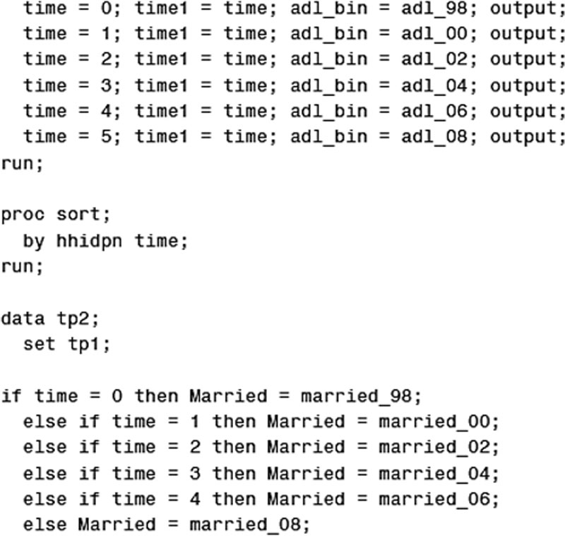
In this empirical illustration, I aim to analyze the effect of an explanatory variable on a binary outcome variable by applying the GEE methodology. Given the requirement of a large sample size to execute GEEs, the AHEAD longitudinal data are used for the analysis (six waves: 1998, 2000, 2002, 2004, 2006, and 2008). The study topic is the effect of current marriage on the presence of disability. Given this research focus, the binary outcome variable is the disability score, with 1 = functionally disabled and 0 = not functionally disabled. This dichotomous variable is created from the ADL count previously indicated. Specifically, a subject is defined as functionally disabled if he or she reports any degree of health-related difficulty in performing activities of daily living, given by ADL_COUNT > 0. As previously mentioned, the ADL count consists of five task items (dress, bath/shower, eat, walk across time, and get in/out of bed). The ADL binary score is measured at the six time points and named ADL_BIN in the analysis. The probability of disability is denoted by Pr(Yij = 1), where i and j indicate subject i at time point j. There are more appropriate approaches for measuring disability in the literature of aging and health studies; the measurement issue of this health indicator, however, is currently not of concern given the focus on an illustration of a statistical technique. The time factor is specified as a continuous variable, for which only the linear component is considered given the results of a preliminary data analysis. The main explanatory variable, marital status, measured at six waves and named Married in the analysis, is the dichotomous variable previously specified, with 1 = currently married and 0 = else. As specified in the linear mixed model on the ADL count, an interaction between time and Married is created. The three centered covariates, “Age_mean,” “Educ_mean,” and “Female_mean,” continue to be used as the control variables.
In the application of GEEs for this analysis, the logit link is specified to indicate the association between the covariates and the binary outcome. The logit model in this context is written as
logit(μij)=logPr(Yij=1)Pr(Yij=0)=X′ijβ,
where
μij is the marginal expectation of the functional disability score for subject
i at time point
j, and the covariate vector
Xij contains six covariates: TIME, Married, TIME × Married, Age_mean, Educ_mean, and Female_mean. In the equation, the
log odds is the transformed outcome variable, assumed to be linearly associated with the covariates. The logit regression model will be further described in
Chapter 10, both generally and with specific regard to longitudinal data analysis.
Here, the issue of centering a dichotomous variable in the application of nonlinear regression models needs to be discussed. In the present illustration, the centered variable of FEMALE is viewed as the expected proportion of women or the propensity score to be a female in the population of interest. In the present regression analysis, it is used to adjust for the effect of a potential confounder on the binary response in a hypothetical population. In predicting the probability for an actual stratum, using a centered dichotomous variable can result in some bias due to functional transformation and retransformation in nonlinear predictions. In such situations, nonlinear predictions should be performed for each stratum separately and then the weighted average of the predicted probabilities should be computed for each observed covariate profile (
Muller and MacLehose, 2014).
As indicated earlier, the GEE estimating function is the score solution for
β when the data follow a log-linear probability distribution. Correlations among subject-specific observations are accounted for by modeling the working correlation matrix. The SAS PROC GENMOD procedure (
SAS, 2012) is applied to estimate population-averaged parameters in nonlinear marginal models given its tremendous flexibility. First, a classical GEE model is created, which uses working correlations to model dependence of repeated measurements of the response for the same subject. The SAS program for this model is displayed.
In SAS Program 9.1, two time variables, TIME and TIME1, are specified due to the use of the time factor as both the categorical and the continuous variables in this GEE model. TIME1, a copy of TIME, is included in the model as the continuous. The binary, time dependent disability score, ADL_BIN, is constructed from the original set of the binary variables, ADL_98 through ADL_08. In the PROC GENMOD statement, the option DESCEND tells SAS to model the probability that Yij = 1. If this option is not specified, the PROC GENMOD procedure models the probability that Yij = 0 as default. In the CLASS statement, the subject’s ID (HHIDPN), MARRIED, and TIME are specified as classification variables, and the PARAM = REF option requests SAS to apply reference cell coding. The specification of a single time factor as two data types is also applied in some other situations. For example, in a linear regression model specifying a unique hybrid covariance matrix, the REPEATED and the RANDOM statements can be specified in the same SAS program. In such cases, two time variables, with exactly the same face values, must be defined simultaneously: one serving as a classification factor included in the CLASS and the REPEATED statements and one used as a continuous variable incorporated in the RANDOM statement.
In the MODEL statement, ADL_BIN is specified as the dependent and the six covariates as the independent variables. Not included in the CLASS statement, TIME1 is specified as a continuous variable in this GEE model. The DIST = BIN option specifies a binomial distribution for the variable ADL_BIN. In the REPEATED statement, the CORR = UNSTR option specifies the covariance structure of the multivariate responses to be unstructured, and the option CORRW requests SAS to display the estimated working correlation matrix. The WITHIN = TIME option specifies the order of repeated measurements within subjects ensuring the observations to be properly ordered and arranged for computing the working correlation matrix. In this step, the time factor needs to be specified as a classification factor, thereby resulting in the specification of two time variables with exactly the face values in the GEE model: one continuous and one categorical.
The analytic results derived from SAS Program 9.1 are displayed in the following output tables.
In SAS Program Output 9.1, the working correlation matrix, given unstructured covariance, is displayed first. There are two distinctive features of this GEE correlation matrix. First, the correlation coefficients in the table suggest that intraindividual repeated measurements are very highly correlated. Therefore, without accounting for correlations among observations for the same subject, the parameter estimates of the regression can be biased and inconsistent. Second, the intraindividual correlation tends to decay consistently over time lag, and the value of correlation is negatively associated with the absolute distance between two time points. As indicated in
Chapter 5, such an autoregressive pattern of correlations in repeated measurements is frequently observed, resulting in the widespread application of the AR(1) or the spatial covariance pattern models in longitudinal data analysis.
Next, the model goodness-of-fit information is reported, which is derived from the two GEE fit criteria described in
Section 9.1.4, QIC(
R) and QIC
u(
R). The values of the two model fit statistics are very close, thereby leading to the same conclusion about the goodness-of-fit for this GEE model.
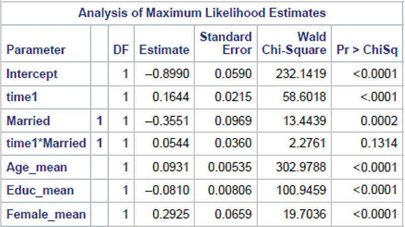
Finally, the parameter estimates, the corresponding standard errors, confidence intervals, z-scores, and p-values are displayed. Time is shown to have a positive, statistically significant effect on disability, as expected. With the currently not married treated as the reference group, current marriage among older persons is negatively associated with the probability of disability, other variables being equal, with its regression coefficient being −0.36 with p < 0.0001. This effect on the logit scale translates into an OR of 0.60, suggesting a 0.40 points reduction in the individual odds of being disabled for a currently married older person as compared to his or her currently not married counterpart. The interaction between TIME and MARRIED is not statistically significant (βtime × married = 0.03, p = 0.45), and therefore, the effect of current marriage on disability is consistent throughout the entire period of time. The effects of the three control variables, all statistically significant (p < 0.0001), are given as: βage = 0.10, OR = 1.11; βedu = −0.08, OR = 0.92; and βfemale = 0.27, OR = 1.31. Interestingly, the effects of the three controls on the logit of ADL_BIN are very close to those on ADL_COUNT.
As indicated earlier, in the classical GEE models, the working correlation matrix of binary data is considered to depend on the means of a categorical data type, thus being constrained in a complicated way. It is perceived that by modeling dependence of repeated measurements with use of conditional OR parameterization, the constraints on the means are relaxed, thereby potentially yielding statistically more efficient, consistent parameter estimates. To examine the validity of this argument, I illustrate a GEE model specifying the log OR for each pair of responses within the same subject for analyzing the association between current marriage and disability in older Americans. For analytic convenience, all subjects are parameterized identically. SAS Program 9.2 specifies a fully parameterized log OR model.
In SAS Program 9.2, all specifications are the same as those in SAS Program 9.1 except for the inclusion of the LOGOR = FULLCLUST option in the REPEATED statement. This option specifies fully parameterized clusters or, in this context, subjects. There is a parameter for each pair of observations, and therefore, there are
n × (
n − 1)/2 parameters in the vector
˜α. In the present analysis, therefore, there are altogether fifteen parameters for the log OR pairs given six time points.
SAS Program 9.2 yields a complete set of results about the estimation. The following output is the parameter information for the GEE model.
In SAS Program Output 2a, the fifteen elements of
˜α correspond to the log OR pairs, with the first number in the parentheses being the order of the row and the second the order of the column. For example, “Alpha5” indicates the log OR between the first and the sixth time points.
Next, the model goodness-of-fit information for the present log OR model is displayed.
This GEE model with log OR parameters yields two model goodness-of-fit information criteria, QIC(R) and QICu(R). Again, the values of the two model fit statistics are very close, pointing to the same conclusion about goodness-of-fit for the analysis. Surprisingly, both the QIC(R) and QICu(R) scores in SAS Program Output 9.2b are moderately higher than those reported in SAS Program Outcome 9.1, thereby suggesting that the GEE model with log OR parameters fits the AHEAD data slightly worse. The following output table displays the analytic results.
The output table displays the parameter estimates, the corresponding standard errors, confidence intervals, z-scores, and p-values. The results for the intercept and the regression coefficients of the four covariates are very close to those estimated from the unstructured working correlation model, with only minor variations. Clearly, for the present analysis, using either the classical or the log OR GEE model generates the same conclusions about the effect of current marriage on disability. Furthermore, the log OR parameters, all statistically significant, suggest that repeated measurements for the same subjects are very highly correlated given the substantial deviations of all the OR pairs from unity. Analogous to the pattern from the classical GEE model, such intraindividual correlations tend to decay consistently over time lag. Clearly, the changing pattern of log OR pairs also results in the same conclusion from the application of the classical GEE model.
Given the similarity of analytic results between the two GEE models, some theoretical questions may be advanced promptly. If the estimated regression coefficients and the goodness-of-fit indices are insensitive to the specification of a more refined covariance matrix, is it necessary to attach a working correlation or an OR matrix in the application of a generalized linear model? According to large-sample theory, the asymptotic limit of
(ˆβ−β0)
, where
b0 is the true coefficient vector, tends to be
0 as the sample size increases. Therefore, the point estimates of the regression coefficients in the standard GLMs are asymptotically unbiased, even with the presence of dependence in repeated measurements of the response for the same subject. Given correlated data, however, the inverse of the observed Fisher information matrix given
ˆβ
does not provide an adequate variance estimator of
ˆβ
(
Liang and Zeger, 1986;
Zeger and Liang, 1986).
With these concerns, next I create a simple logistic regression model on the relationship between marital status and disability. By doing so, the estimated regression coefficients and the corresponding standard errors from the “naïve” logistic regression model can be compared to those from the two GEE models. The following is the SAS program for this logistic model.
In SAS Program 9.3, the PROC LOGISTIC statement calls for the application of the logistic regression procedure. Other statements and options have the same interpretations as those in the PROC GENMOD procedure. Without any repeated or random components, this logistic regression model yields the regression coefficient estimates without adjusting dependence of repeated measurements for the same subject. The following output presents the MLE solution for the regression coefficients and other statistics.
SAS Program Output 9.3 displays the estimated regression coefficients, standard errors, and p-values for the intercept and the six covariates. Compared to the results from the two GEE models, there are some changes in the point estimates, particularly the estimated regression coefficients of TIME1 and TIME1 × MARRIED. Surprisingly, the estimated standard errors from the “naïve” model are fairly close to those of the GEEs, more so than between the two sets of the regression coefficients. Therefore, the p-values of the regression coefficient estimates result in identical test results to those from the GEEs.

 (9.1)
(9.1) (9.2)
(9.2) (9.3)
(9.3)


 (9.4)
(9.4) (9.6)
(9.6)
 (9.8)
(9.8)
 (9.9)
(9.9) (9.10)
 (9.11)


 (9.27)
 (9.28)
 (9.29)