
Nonlinear Control Algorithms with Integral Action*
Abstract
Popular nonlinear controllers are composed of proportional and derivative terms (or their combination). Sometimes when the system is constantly disturbed, the controllers are not capable of achieving the desired position. The integral part in a control scheme is often used to reduce this behavior even in the presence of uncertainties or perturbations; furthermore, when the disturbance is constant, the steady state error converges to zero. In this chapter classical controllers used in the aerial vehicles community are developed with an integral part to stabilize a VTOL (Vertical Take-Off and Landing) aircraft. The proposed algorithms are validated in simulations and real flight missions using a quadcopter test-bed. The main results, presented in several graphs, illustrate good performance of the closed-loop system.
Keywords
Nonlinear algorithms; Integral term; Lyapunov stability; Flight tests; Quadcopter vehicle
Working with UAVs (Unmanned Aerial Vehicles) is not an easy task. Sometimes when researchers or students propose controllers, the most popular suggestion is to use linear controllers like feedback or PD (Proportional-Derivative) controllers. In some cases, to correctly apply these controllers, it is necessary to modify the nonlinear mathematical equations using some assumptions, to develop a simplified nonlinear or even, in the best case from a control design point of view, a linear model. The latter for some researches is inconceivable; nevertheless, it gives an easier way to understand the system redline in several cases. Linearizing the quadcopter model is not a problem because, when the vehicle is hovering using small angle movements to perform a trajectory, its dynamics are strongly simplified and resemble a linear system. In general, two integrators or four integrators in cascade are the most used linear models.
Even if the linear mathematical equations are used, this does not signify that the controller has to be linear. There exist several control algorithms conceived from linear models but directly applied to nonlinear systems. And when such a controller is validated in real time, it captures the attention of the UAV community.
In addition, it is common in practical applications, such as the stabilization at a given position, that the closed-loop system performance is degraded and the states do not converge to the desired values when model uncertainties or unknown constant perturbations are present. The main motivation for this chapter is to improve the behavior of the popular control schemes by adding an integral part.
6.1 From PD to PID Controllers
The simplest mathematical representation of the attitude of a VTOL vehicle (quadcopter included) is given by two integrators in cascade. From (5.7) we can deduce that1
where η defines an Euler angle (yaw, pitch, or roll), ![]() represents the control input, and
represents the control input, and ![]() stands for an unknown perturbation.
stands for an unknown perturbation.
Stabilizing the previous system is an easy task: in general, the disturbance is neglected and then a PD controller is enough. Then we propose taking
with ![]() defining the proportional gain,
defining the proportional gain, ![]() the derivative gain, and
the derivative gain, and ![]() being the error between the state η and its desired value
being the error between the state η and its desired value ![]() . Notice in Fig. 6.1 that with
. Notice in Fig. 6.1 that with ![]() the control law stabilizes the system (solid line). Stability analysis of the closed-loop system is obvious and not necessary to develop here. For simulation purposes the initial conditions were
the control law stabilizes the system (solid line). Stability analysis of the closed-loop system is obvious and not necessary to develop here. For simulation purposes the initial conditions were ![]() and
and ![]() . Nevertheless, if
. Nevertheless, if ![]() , a steady state error could be observed, see Fig. 6.1-dotted line (for simulation,
, a steady state error could be observed, see Fig. 6.1-dotted line (for simulation, ![]() ). The previous problem can be solved by adding an integral term to the controller, see Fig. 6.3. This control algorithm is known as a PID controller (proportional-integral-derivative).
). The previous problem can be solved by adding an integral term to the controller, see Fig. 6.3. This control algorithm is known as a PID controller (proportional-integral-derivative).

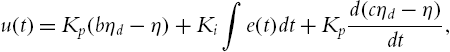
The PID controller is by far the most common control algorithm used in industrial processes [1]. The most popular expression for this algorithm is

where ![]() defines the integral gain. Its diagram representation is illustrated in Fig. 6.2.
defines the integral gain. Its diagram representation is illustrated in Fig. 6.2.

From Fig. 6.2 notice that the error expression is

and it can be concluded that, as the control law has an integral term, ![]() .
.
There exist several expressions derived from (6.2), for example, the PID with set-point weighting algorithm is becoming popular because it can be deduced as a regulator with 2 DOF (Degrees Of Freedom), namely
where ![]() represents the set-point and η is the measurement variable. The response to the set-point changes will depend on the magnitudes of b and c while its stability and robustness with respect to perturbations and the measurement noise will be the same as that for the algorithm without set-point weighting (6.2).
represents the set-point and η is the measurement variable. The response to the set-point changes will depend on the magnitudes of b and c while its stability and robustness with respect to perturbations and the measurement noise will be the same as that for the algorithm without set-point weighting (6.2).
Notice that, when controlling the quadcopter attitude, it is possible to measure the angular rate ![]() . In this way, from (6.3) and with
. In this way, from (6.3) and with ![]() and
and ![]() , we get
, we get

In Fig. 6.3, it can be observed how the attitude performance is restored when using a PID controller. Following these ideas, the goal of this chapter is to introduce two nonlinear controllers having integral terms to stabilize the quadcopter system or only some of its dynamics.

6.2 Saturated Controllers with Integral Component
The purpose of this section is to present a summary of the control algorithms based on saturation functions with integral action to stabilize a quadcopter represented by a chain of integrators in cascade2. A detailed version of this result can be found in [2].
The algorithms stabilize a chain of integrators of n states described by

or, in the classical form, by
with

where ![]() defines the states of the system,
defines the states of the system, ![]() is called the input,
is called the input, ![]() represents the state matrix, and
represents the state matrix, and ![]() denotes the input matrix. An essential element of these control laws is the saturation function that can be defined as follows.
denotes the input matrix. An essential element of these control laws is the saturation function that can be defined as follows.
Definition 6.1
Given a positive constant b, a function ![]() is said to be a linear saturation for s if it is continuous and nondecreasing function satisfying:
is said to be a linear saturation for s if it is continuous and nondecreasing function satisfying:
• ![]() for all
for all ![]() ,
,
• ![]() for
for ![]() ,
,
• ![]() for
for ![]() .
.
Several controllers have been proposed using saturation functions to stabilize system (6.5); see, for example, [3–5]. Nevertheless, these controllers did not include an integral term. In the following, three main configurations of nonlinear controllers based on saturation functions with an integral part are presented. For the stability analysis the following change of coordinates is necessary:

Then (6.5) yields
where ![]() ,
, ![]() , and
, and ![]() . Indeed, the stability of system (6.6) implies the stability of system (6.5).
. Indeed, the stability of system (6.6) implies the stability of system (6.5).
6.2.1 Nested Saturation with Integral Part Controller – NSIP
The following controller asymptotically stabilizes system (6.6):
where

Notice that ![]() is the binomial coefficient.
is the binomial coefficient.
Stability Analysis
Rewriting (6.7) as
we can deduce that ![]() for
for ![]() which will be defined later to assure convergence. Take
which will be defined later to assure convergence. Take ![]() , then
, then ![]() . If
. If ![]() then
then ![]() and so for
and so for ![]() we obtain
we obtain ![]() . This proves that (6.7) stabilizes system (6.6) for
. This proves that (6.7) stabilizes system (6.6) for ![]() . The next step is to prove that the same is also true for
. The next step is to prove that the same is also true for ![]() . We propose
. We propose ![]() and hence
and hence ![]() . To compute
. To compute ![]() remember that3
remember that3

then

with ![]() , and therefore
, and therefore ![]() . As
. As ![]() , if
, if ![]() ,
, ![]() which implies that
which implies that ![]() and
and ![]() such that
such that ![]() ,
, ![]() . Therefore, if
. Therefore, if ![]() , it follows that
, it follows that
So we proved that the closed loop (6.6)–(6.7) is stable for ![]() , then, using the recurrence theorem, (6.6)–(6.7) holds
, then, using the recurrence theorem, (6.6)–(6.7) holds ![]() .
.
From the previous analysis we have that ![]() and the last positive-definite function is
and the last positive-definite function is ![]() ; therefore,
; therefore, ![]() , which implies that
, which implies that ![]() and
and ![]() goes to zero. Hence, from the definition of
goes to zero. Hence, from the definition of ![]() , we have that
, we have that ![]() . If we assume that
. If we assume that ![]() as
as ![]() which implies that
which implies that ![]() , then for
, then for ![]() it follows that
it follows that ![]() and then
and then ![]() . This means that
. This means that ![]() as
as ![]() . Finally, as
. Finally, as ![]() tends to zero, using the recurrence theorem, we obtain
tends to zero, using the recurrence theorem, we obtain ![]() as
as ![]()
![]() . Observe that as
. Observe that as ![]() ,
, ![]() .
.
From the above, we notice that ![]() for
for ![]() . This implies that
. This implies that ![]() also goes to zero. Now we have that
also goes to zero. Now we have that

Analyzing the previous equation, we can deduce that ![]() contains
contains ![]() variables,
variables, ![]() . It was proved that these variables converge to zero, so the above implies that
. It was proved that these variables converge to zero, so the above implies that ![]() also goes to zero, and we can conclude that every
also goes to zero, and we can conclude that every ![]() goes to zero.
goes to zero.
6.2.2 Separated Saturation with Integral Part Controller – SSIP
The following controller stabilizes system (6.6) globally asymptotically:
where

Stability analysis is similar to that proposed for the NSIP algorithm, the main difference is the saturation constraints required to perform the Lyapunov analysis and defined as
6.2.3 Saturated State Feedback with Integral Part Controller – SSFIP
The following controller can be seen as a PID algorithm with bounded states. The algorithm has the form

where ![]() denotes the state i and
denotes the state i and ![]() is the constant gain controller. This control law stabilizes system (6.5) globally asymptotically. For the stability analysis, we rewrite (6.12) in the following form:
is the constant gain controller. This control law stabilizes system (6.5) globally asymptotically. For the stability analysis, we rewrite (6.12) in the following form:

Rewrite (6.13) for ![]() as
as
with ![]() and define
and define

Propose ![]() , and then
, and then ![]() . Assuming that
. Assuming that ![]() , we get
, we get ![]() which implies that
which implies that ![]() . Thus, there exist a time
. Thus, there exist a time ![]() such that
such that ![]() ,
, ![]() and, as a consequence,
and, as a consequence, ![]() .
.
It is assumed that for a given l, (6.13) is true and ![]() is bounded
is bounded ![]() and
and ![]() . Now, we prove that (6.13) is also true for
. Now, we prove that (6.13) is also true for ![]() . Take
. Take ![]() , then
, then ![]() . We have that
. We have that ![]() , and then
, and then ![]() . Therefore
. Therefore ![]() .
.
The above implies

Assuming ![]() gives
gives ![]() , hence
, hence ![]() . Notice that
. Notice that ![]() and
and ![]() is bounded. Thus, if
is bounded. Thus, if ![]() , then
, then ![]() . Therefore
. Therefore ![]() and
and ![]() such that
such that ![]() ,
,

Since it was proved that (6.13) is true for ![]() , using the recurrence theorem, the same is also true
, using the recurrence theorem, the same is also true ![]() . This means that for
. This means that for ![]() there exists a time
there exists a time ![]() such that
such that

The previous equations hold if the following conditions are satisfied: ![]() ,
, ![]() ;
; ![]() ,
, ![]() ,
, ![]() ;
; ![]() ,
, ![]() .
.
Observe that for ![]() the closed-loop system is
the closed-loop system is ![]() and, as
and, as ![]() is Hurwitz, stability is proved.
is Hurwitz, stability is proved.
The previous stability analysis demonstrated the convergence of the states to zero, ![]() , implying
, implying ![]() . Nevertheless, we can consider system (6.6) as an error system such that
. Nevertheless, we can consider system (6.6) as an error system such that ![]() , with
, with ![]() ; and then this implies that
; and then this implies that ![]() and
and ![]() . The previous holds for
. The previous holds for ![]() constant or bounded
constant or bounded ![]() .
.
More details about the previous controllers can be found in [2].
6.2.4 Validation in a Quadcopter Vehicle
The control algorithms were validated in simulations using the simplified quadcopter model described in Sect. 5.1.5 of Chap. 5. To develop the algorithms, the following hypotheses were used:
• ![]()
• quasi-stationary movements
• no external and unknown disturbances present
Notice from the equations in the simplified model that the altitude and the attitude can be represented by two integrators in cascade as
where z is the altitude of the aerial vehicle, ψ the yaw angle, ![]() defines the control input for the yaw angle, and
defines the control input for the yaw angle, and ![]() , where
, where ![]() denote the pitch and roll angles, g expresses the gravitational acceleration, and u represents the main control input.
denote the pitch and roll angles, g expresses the gravitational acceleration, and u represents the main control input.
Due to chapter-length limitation, we only use the SSFIP algorithm; similar results can be obtained using the NSIP and SSIP algorithms. Therefore the control scheme to stabilize the previous system takes the form

Once the altitude and the yaw movement are stabilized, the next step is to stabilize the longitudinal and lateral dynamics. They are typically coupled and both have high impact on the complete vehicle dynamics. Thus their classical simple representation is denoted by four integrators in cascade in the following form

where s defines the state x or y, and ρ represents the angle θ or ϕ, respectively. Notice that the controller needs to be developed for a linear system. Then linearizing the above, it follows that ![]() . Using the proposed methodology, the controller SSFIP for the previous system is
. Using the proposed methodology, the controller SSFIP for the previous system is

with ![]() and
and ![]() being the desired position. Remark that for the longitudinal model
being the desired position. Remark that for the longitudinal model ![]() , and consequently for the longitudinal case, the last three terms of the above expression are positive.
, and consequently for the longitudinal case, the last three terms of the above expression are positive.
6.2.4.1 Simulation Results
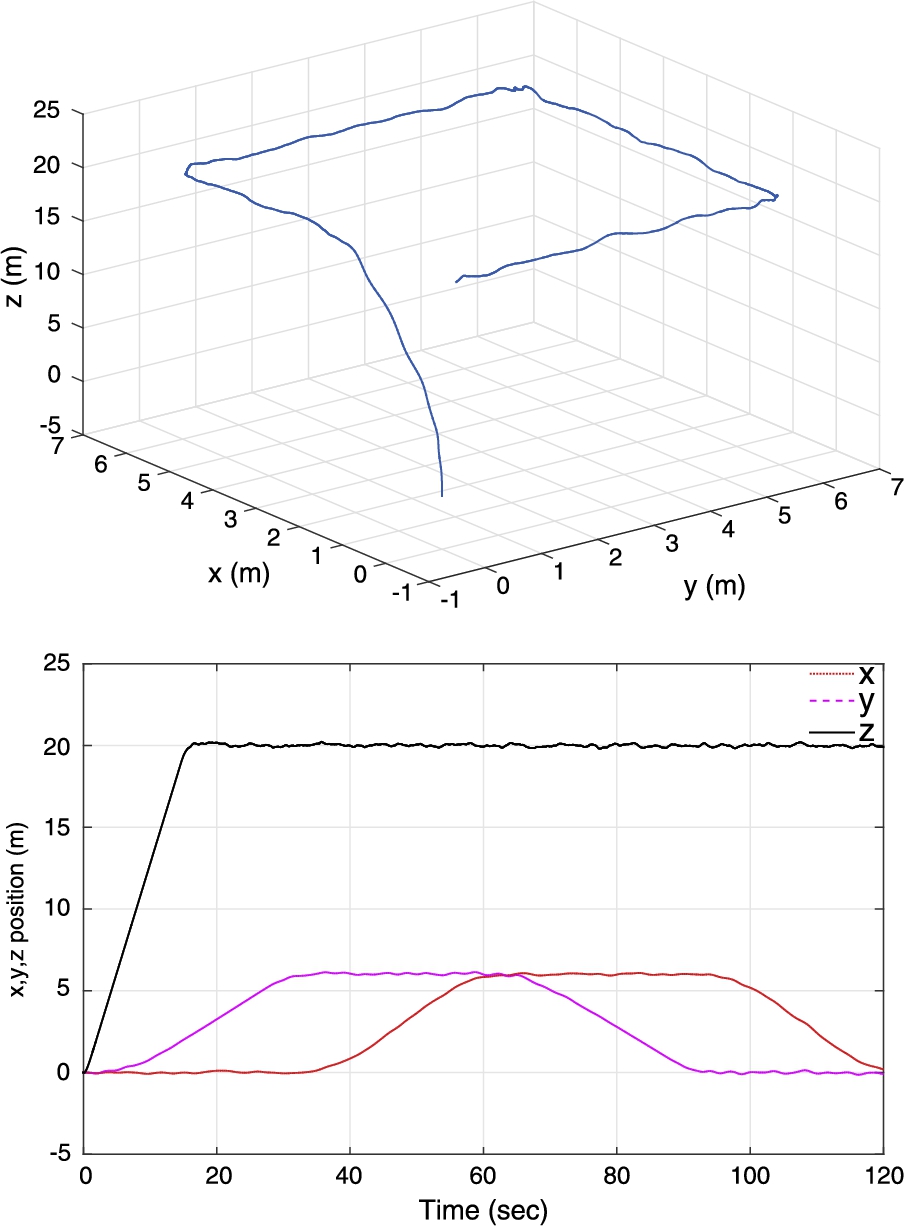
The simulation objective is to accurately follow a desired trajectory in the presence of uncertainties (white noise) in the states ![]() , and z. The following graphs introduce good behavior when applying the SSFIP control to the quadcopter system, see Figs. 6.4–6.7. Notice the good performance of the closed-loop system, the boundedness of the states, and the smallness of control responses. Observe also that only the θ and ϕ angles are affected by the uncertainties; this fact is normal because the noise in the x or y axis produces uncertainties in the longitudinal or lateral dynamics. The desired altitude is
, and z. The following graphs introduce good behavior when applying the SSFIP control to the quadcopter system, see Figs. 6.4–6.7. Notice the good performance of the closed-loop system, the boundedness of the states, and the smallness of control responses. Observe also that only the θ and ϕ angles are affected by the uncertainties; this fact is normal because the noise in the x or y axis produces uncertainties in the longitudinal or lateral dynamics. The desired altitude is ![]() , and in the horizontal plane the desired trajectory is to follow a square trajectory with 6 m on each side. The initial conditions were zero for all the states except for the yaw angle which was
, and in the horizontal plane the desired trajectory is to follow a square trajectory with 6 m on each side. The initial conditions were zero for all the states except for the yaw angle which was ![]() grad.
grad.

 responses, the initial condition for yaw was 10 grad.
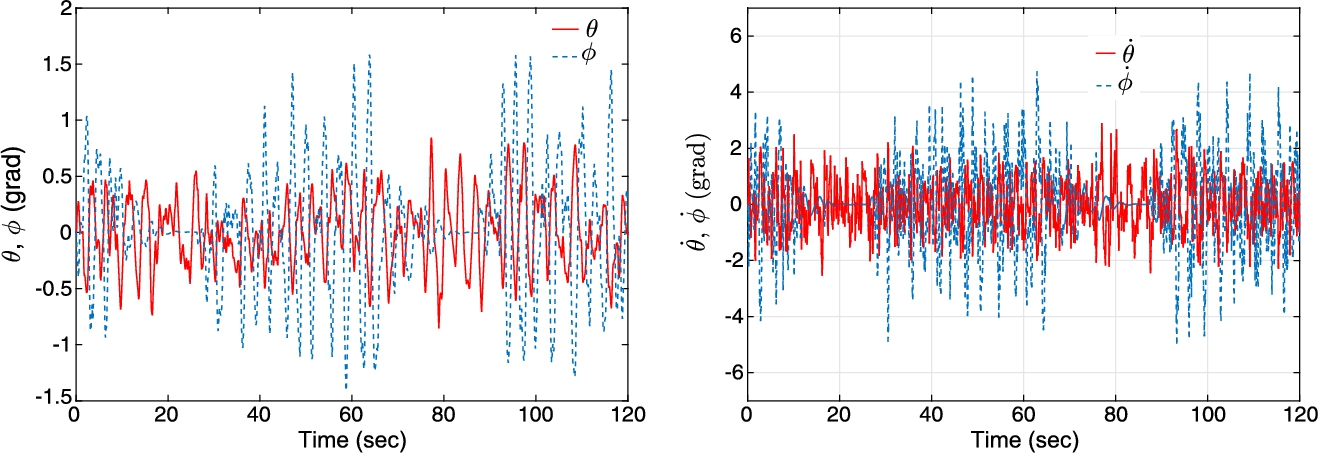

6.3 Integral and Adaptive Backstepping Control – IAB
The next controller is developed using the quadcopter model defined in Sect. 2.3 of Chap. 2. Introducing uncertainties in the model, Eqs. (2.17)–(2.18) become
where ξ defines the position of the quadrotor, ![]() and
and ![]() express the thrust and torque vectors generated by the rotation of helices,
express the thrust and torque vectors generated by the rotation of helices, ![]() denotes the gravity force. R is the rotation matrix, Ω introduces the angular velocity, and I represents the inertia matrix of the quadrotor. The terms
denotes the gravity force. R is the rotation matrix, Ω introduces the angular velocity, and I represents the inertia matrix of the quadrotor. The terms ![]() and
and ![]() define the non-modeled dynamics and the perturbations of the aerial vehicle (drag effects included).4
define the non-modeled dynamics and the perturbations of the aerial vehicle (drag effects included).4
Adding an integral term in the classical backstepping approach increases the robustness of the closed-loop system. In addition, in this algorithm an adaptive sense is introduced, i.e., the adaptive part will help to estimate some unknown parameters and to counteract them.
6.3.1 Quadcopter IAB Algorithm
To stabilize the quadcopter, let us define the position error as follows:
Now propose a positive definite function to design a virtual velocity ![]() that will ensure the convergence to the desired position5
that will ensure the convergence to the desired position5
where ![]() represents the inner vector product,
represents the inner vector product, ![]() is a positive constant matrix, and
is a positive constant matrix, and ![]() . Differentiating
. Differentiating ![]() results in
results in ![]() , and taking the virtual velocity as
, and taking the virtual velocity as ![]() , with
, with ![]() a positive constant matrix, gives
a positive constant matrix, gives
Define the velocity error as
with ![]() . Now a positive definite function is proposed to ensure convergence of the position error to zero
. Now a positive definite function is proposed to ensure convergence of the position error to zero
From the velocity error definition, it follows that ![]() , and then the above can be expressed as
, and then the above can be expressed as ![]() , by choosing
, by choosing
with ![]() denoting a positive constant matrix and
denoting a positive constant matrix and ![]() the estimated value of
the estimated value of ![]() . Rewriting
. Rewriting ![]() , it follows that
, it follows that
with ![]() . Suppose that
. Suppose that ![]() is constant, thus
is constant, thus ![]() . Consider the following candidate Lyapunov function
. Consider the following candidate Lyapunov function ![]() , with
, with ![]() being a positive diagonal constant matrix. Then
being a positive diagonal constant matrix. Then
Now propose ![]() as the desired dynamics for
as the desired dynamics for ![]() . Thus
. Thus
There exists a relationship between u, the main force ![]() , and the quadcopter attitude η so that it is possible to find
, and the quadcopter attitude η so that it is possible to find ![]() from
from ![]() . Here the z–y–x Euler convention is used. Consequently, the rotation matrix, R, has the following form:
. Here the z–y–x Euler convention is used. Consequently, the rotation matrix, R, has the following form:
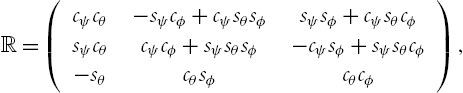
where the c and s stand for the cosine and sine functions, respectively. From (6.19) and (6.23), the following relations for ![]() can be obtained:
can be obtained:


![]() is assigned arbitrarily, and the main thrust is taken as
is assigned arbitrarily, and the main thrust is taken as ![]() . Let us define the error of Euler angles as
. Let us define the error of Euler angles as
Propose the next positive definite function ![]() , where
, where ![]() is a positive constant matrix and
is a positive constant matrix and ![]() . Thus,
. Thus, ![]() . Define the virtual angular velocity as
. Define the virtual angular velocity as ![]() , with
, with ![]() being a positive constant matrix. This implies
being a positive constant matrix. This implies
Define the angular velocity error as ![]() . Remember that
. Remember that ![]() , then
, then ![]() . Propose the following positive definite function,
. Propose the following positive definite function, ![]() , then get
, then get
Choose the control input as
with ![]() being a positive constant matrix and
being a positive constant matrix and ![]() the estimated value of
the estimated value of ![]() . Then
. Then
with ![]() . Consider
. Consider ![]() constant, then
constant, then ![]() . Propose the following candidate Lyapunov function,
. Propose the following candidate Lyapunov function, ![]() , where
, where ![]() is a positive diagonal constant matrix. It implies that
is a positive diagonal constant matrix. It implies that
Define ![]() as the desired dynamics for
as the desired dynamics for ![]() . Thus
. Thus
6.3.2 Simulation with Perturbations
Several simulations were carried out to validate the IAB control. The simulation parameters are written in Table 6.1, these parameters take into account the characteristics of the Quadcopter Flexbot platform shown in Table 6.2. In Fig. 6.8, the performance of the closed-loop system response can be observed. In this simulation no perturbations were considered. The desired mission was to realize a circle trajectory of radius 1 m and altitude of 1 m. To keep the chapter of acceptable length, only the quadcopter's position responses are presented.
Table 6.1
Simulation parameters
| Parameter | Value | Parameter | Value |
| I | diag(8,8,6)⋅10−4 | g | 9.81 |
| ξ ref |
|
|
diag(1,1,1)⋅0.35 |
|
|
diag(1,1,1)⋅16 |
|
diag(1,1,1)⋅2 |
|
|
diag(1,1,1)⋅16 | Γ1 | diag(1,1,1)⋅57 ⋅ 10−4 |
| Γ2 | diag(32,32,24)⋅10−6 |
|
diag(1,1,1)⋅0.05 |
|
|
diag(1,1,1)⋅0.1 | Initial conditions | Zero |

Table 6.2
Quadcopter flexbot parameters
| Parameter | Value |
| Mass | 0.057 kg |
| Payload | 0.023 kg |
| Max diameter | 0.12 m |
| Helix length | 0.05 m |

The next simulation takes into account two perturbations when the UAV is following a circular trajectory. One of them considers an extra torque which could arise from a displacement of its battery from the gravity center of the vehicle. The other considers the vehicle moving in the presence of a crosswind which produces an external force acting on the quadcopter. The force perturbation ![]() represents about 25% of the vehicle weight, and the torque perturbation
represents about 25% of the vehicle weight, and the torque perturbation ![]() is about the 25% of the total torque that quadcopter can manage. The systems response can be appreciated in Figs. 6.9 and 6.10. Notice that even if there are perturbations in the system, the controller stabilizes the desired position well. The estimates of perturbations are presented in Fig. 6.10. As before, notice that the adaptive part estimates the unknown perturbations well.
is about the 25% of the total torque that quadcopter can manage. The systems response can be appreciated in Figs. 6.9 and 6.10. Notice that even if there are perturbations in the system, the controller stabilizes the desired position well. The estimates of perturbations are presented in Fig. 6.10. As before, notice that the adaptive part estimates the unknown perturbations well.


6.3.3 Simulation with Inaccurate Mass
Other simulations were realized to validate the performance of the controller when the vehicle mass is changing (it could be that the vehicle is transporting an object). Then the next simulation introduces the behavior of the vehicle which is tracking a circular trajectory and after a certain time it drops the object it was carrying. In simulation, the object represents 25% of the initial mass and is dropped at 40 seconds. The presence of perturbations of the same magnitudes as before is considered as well, see Fig. 6.11. Notice here that the controller is capable of stabilizing the vehicle and tracking the trajectory even in the presence of perturbations and with a mass loss. In Fig. 6.12 the estimates of perturbations are illustrated. Observe that the effect of weight loss is included in the force estimates.


6.3.4 Experimental Results
The integral adaptive backstepping algorithm proposed previously was validated in flight tests. Three experiments were carried out to observe the performance of the closed-loop system. The first one was to follow a circular trajectory, the second experiment consisted in stabilizing the aerial vehicle at hover, and the last flight test was to keep the vehicle hovering in the presence of external and unknown wind. The vehicle used in the experiments was a quadcopter with the parameters shown in Table 6.3. A radio antenna was added to the quadrotor in order to get access to the torques estimated by the adaptive algorithm in the platform. This antenna weighs 15 g and was placed in one arm of the vehicle in order to generate the torque perturbation.
Table 6.3
Quadcopter parameters
| Parameter | Value |
| Mass | 0.257 kg |
| Payload | 0.070 kg |
| Max diameter | 0.20 m |
| Helix length | 0.125 m |
|
|
diag(8,8,6)⋅10−2 |
Circular Trajectory
The reference path is a circle of 0.8 m radius whose center is at ![]() , the result can be seen in Fig. 6.13.
, the result can be seen in Fig. 6.13.

Fig. 6.14 shows the estimates of the force and torque perturbations, respectively. These estimates take into account the dynamics not modeled, as well the additional torque generated by the antenna.

Stabilization at Hover
In this experiment the objective was to maintain the quadcopter at hover, the desired position was ![]() . Figs. 6.15 and 6.16 describe the behavior of the vehicle during the test.
. Figs. 6.15 and 6.16 describe the behavior of the vehicle during the test.


Hover with External Perturbations
In this section the last experiment is repeated; however, in this case a disturbance is introduced by a wind gust generated with a fan for ![]() . Figs. 6.17–6.18 show the behavior of the quadrotor. We remark that the estimates and Euler angles oscillate more because they try to compensate the perturbations introduced in this experiment.
. Figs. 6.17–6.18 show the behavior of the quadrotor. We remark that the estimates and Euler angles oscillate more because they try to compensate the perturbations introduced in this experiment.


6.4 Discussion
Two control algorithms containing an integral term were proposed to stabilize or navigate an aerial vehicle. Saturation functions were used to conceive three nonlinear control laws and applied to stabilize a quadcopter vehicle. Simulation results indicated good performance of the closed-loop system when following a desired trajectory. The control inputs and states were bounded without degrading the vehicle performance.
The second controller is based on the backstepping approach to propose an integral and adaptive nonlinear control law. This controller was also applied to the quadcopter vehicle and validated in simulation and real-time flight tests. Three cases were studied and analyzed to demonstrate good behavior of the closed-loop system. Simulations and experimental results demonstrated this fact.