
Delay Signals & Predictors*
Abstract
Predictive algorithms have been seen as theoretical contributions without possible real-time validation for several years due to their difficult implementation in real systems. Delays are present when working with aerial drones due to different sampling periods coming from sensor measurements and/or when computing the control schemes. These delays sometimes are big enough, and the system could become unstable. In this chapter, two schemes based on predictors are proposed and validated in real time. The first improves the attitude of a VTOL aircraft while the second compensates delays in the control input. Results are illustrated with some graphs showing good performance of the closed-loop system.
Keywords
Delay systems; Predictive algorithms; Quadcopter; Practical validation
Several control algorithms aiming at stabilization of aerial vehicles can be found in the literature [1,2]. Some of these control/navigation strategies have been applied in real time using efficient but expensive sensing systems [3]. Other research teams use commercial sensors combined with observer/predictor algorithms that improve measurements [4]. Whatever the case, a common problem when applying control strategies in real time is the measurement delay represented as input delays. When these delays are significant, the performance of the closed-loop system suffers and a crash may occur.
In the past, the control of linear processes with time delay in either the input or output has been addressed with strategies such as the Smith Predictor (SP) [5] and the Finite Spectrum Assignment (FSA) [6]. The Smith Predictor [5] can be considered as the first predictor-based control for SISO (Single-Input Single-Output) open-loop stable linear systems [7]. Later the same concept was extended for MIMO (Multiple-Input Multiple-Output) open-loop unstable systems by introducing an h units of time ahead state predictor [6,8]. The original proposals to deal with time-delay systems suffer from robustness problems and implementation issues (a good survey can be found in [9]). In [10] a discrete predictor for continuous-time plants with time delay is proposed, and the closed-loop stability is proved. More recently, in [11], the robustness of the proposed predictor was proved with respect to a delay mismatch or model uncertainties [12], and also to perform well in combination with a state observer [13]; the issue of time-varying delays was also addressed in [14]. Provided that nowadays almost any control system application is implemented using a computer, discrete-time control schemes are more interesting in practical applications [15].
This chapter presents an observer–predictor algorithm (OP-A) which is used to counteract the inherent delays in the attitude estimates. The origin of such delays is discussed and illustrated by comparing the measurements of a commercial IMU (Inertial Measurement Unit) with those coming from optical encoders. The OP-A is used to improve the estimation of the pitch and roll angles, and it is based on a Kalman Filter (KF) and a discrete-time predictor to fuse the measurements coming from gyroscopes and accelerometers. The topic of time delay systems is reviewed before introducing a discrete-time predictor and a state predictor which is based on the Fundamental Calculus Theorem and the Backstepping approach. The advantages of using predicted measurements is demonstrated in simulations and in real-time experiments.
4.1 Observer–Predictor Algorithm for Compensation of Measurement Delays
As aforementioned, the IMUs are the core of lightweight aerial robotic applications as they provide attitude estimates and angular velocity measurements. In practice it is observed that the attitude estimated by an IMU exhibits a delay with respect to its real value. This fact is more significant when using low-cost sensors. Since low-cost devices have typically worse noise performance, their signals must be filtered at lower frequencies, thus introducing larger delays. In any case, even high-performance IMUs provide delayed measurements. In order to illustrate this fact, the experimental platform described in Sect. 3.3.6.1 of Chap. 3 is used to compare the angular measurements against a commercial IMU (Mircrostrain 3DM-GX2) with those of coming from a set of encoders which are faster and more accurate than any IMU. A zoom of the comparison is represented in Fig. 4.1 where a delay of approximately 40 ms is appreciated.

One of the unavoidable sources of delay is the low-pass filtering before sampling. During the data acquisition process in an IMU, the signals are low-pass filtered to remove noise and avoid aliasing effects. Another issue is the computational time required to run the estimation algorithm which is often carried out in an onboard microcontroller. The incorporation of delayed measurements into the Kalman filter while preserving optimality is far from being trivial. When the delay consists of only a few sample periods, the problem can be handled optimally by augmenting the state vector [16]. However, for larger delays the computational burden of this approach becomes too large. This topic has been investigated in [17]. More recent work on this topic has been done in [18] where a general delayed KF framework is derived for linear time-invariant systems.
4.1.1 The Finite Spectrum Assignment Problem
Let us consider the following time-delay systems:

where the time delay τ affects either the input or the output. Notice that, under the feedback control law ![]() , both systems are equivalent in terms of stability. To be more specific, such a control law acting on the systems in (4.1) leads to
, both systems are equivalent in terms of stability. To be more specific, such a control law acting on the systems in (4.1) leads to
which has an infinite-dimensional characteristic equation ![]() . This equation (quasipolynomial) is transcendental, which makes it very difficult to solve. Moreover, if the system has uncertainties, the solution becomes even more complicated. Therefore, it would be convenient to get rid of the delay in the characteristic equation, so that conventional analysis and design techniques could be applied.
. This equation (quasipolynomial) is transcendental, which makes it very difficult to solve. Moreover, if the system has uncertainties, the solution becomes even more complicated. Therefore, it would be convenient to get rid of the delay in the characteristic equation, so that conventional analysis and design techniques could be applied.
It is well known that for the systems in (4.1), the feedback control law

yields the closed-loop characteristic equation ![]() ; see [6]. The finite spectrum assignment (FSA) feature of this control law is a significant advantage from a design point of view. However, the practical implementation of the distributed control law (4.3) has raised several problems. A reasonable approach consists in using a numerical quadrature rule to approximate the integral term. It has been shown in [19] that the control law (4.3) with a large discretization step size may not stabilize the systems in (4.1). A safe implementation of the controller (4.3) was introduced in [20], based on including a low-pass filter in the control loop. In the next section, the discrete-time predictor presented in [10] is developed and proved to be suitable for open-loop unstable time-delay systems, robust with respect to a delay mismatch [11], or model uncertainties [12].
; see [6]. The finite spectrum assignment (FSA) feature of this control law is a significant advantage from a design point of view. However, the practical implementation of the distributed control law (4.3) has raised several problems. A reasonable approach consists in using a numerical quadrature rule to approximate the integral term. It has been shown in [19] that the control law (4.3) with a large discretization step size may not stabilize the systems in (4.1). A safe implementation of the controller (4.3) was introduced in [20], based on including a low-pass filter in the control loop. In the next section, the discrete-time predictor presented in [10] is developed and proved to be suitable for open-loop unstable time-delay systems, robust with respect to a delay mismatch [11], or model uncertainties [12].
4.1.2 An h-Step Ahead Predictor
As discussed in the introduction of the chapter, in a quadrotor vehicle, the estimated variables are unavoidably affected by small time delays which can be counteracted by using a predictive feedback. As it can be seen in (4.3), for the implementation of the predictive control law, a model of the system is needed. The rotational dynamics of the quadrotor using the Newton–Euler approach are given by (2.8). It has been showed in several works (and corroborated in flight tests) that, under some circumstances, the rotational dynamics of the quadrotor can be reduced to a double integrator on each axis
where ![]() is the orientation of the vehicle,
is the orientation of the vehicle, ![]() is a control transformation, τ is the vector of external torques, and
is a control transformation, τ is the vector of external torques, and ![]() is the inertia matrix. In the simplified model (4.4), the axes are decoupled, and each of them can be represented in a discrete-time state-space form
is the inertia matrix. In the simplified model (4.4), the axes are decoupled, and each of them can be represented in a discrete-time state-space form

where ![]() ,
, ![]() , and
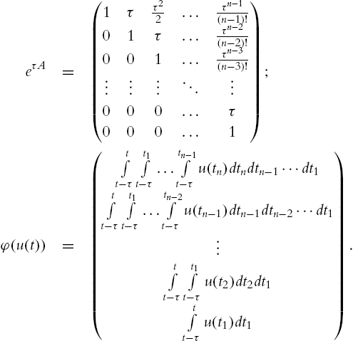
, and ![]() is the sampling period. The discretized matrices have been obtained using
is the sampling period. The discretized matrices have been obtained using

Notice that for the assumed simplified model (4.4), the matrix ![]() is nilpotent with
is nilpotent with ![]() for any
for any ![]() , and thus there is no discretization error because the truncated expansion of the exponential matrix is exact.
, and thus there is no discretization error because the truncated expansion of the exponential matrix is exact.
Let us as assume now that the state of the plant is fully accessible, but there is a known constant transmission delay τ which is approximated1 to be a multiple of the sampling period ![]() , that is,
, that is, ![]() with
with ![]() . The measured delayed state is denoted by
. The measured delayed state is denoted by
The source of the measurement ![]() can be the output of some of the estimation algorithms presented in Chap. 3. If a conventional state feedback
can be the output of some of the estimation algorithms presented in Chap. 3. If a conventional state feedback ![]() is used to stabilize (4.5), the resulting closed-loop system will be
is used to stabilize (4.5), the resulting closed-loop system will be ![]() . Such a system may have poor performance or even become unstable if d is sufficiently large. This is especially critical for open-loop unstable systems, as is the case for quadrotor vehicles.
. Such a system may have poor performance or even become unstable if d is sufficiently large. This is especially critical for open-loop unstable systems, as is the case for quadrotor vehicles.
In order to counteract the effect of the measurement delay, an h-step ahead predicted state is obtained by using (4.5) recursively to propagate the state of the system. Notice that
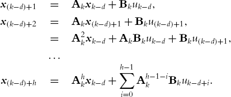
Taking into account the definition of the delayed measurement in (4.7), the predicted state is defined by

with the prediction horizon ![]() being a design parameter. Notice that choosing
being a design parameter. Notice that choosing ![]() (assuming perfect model matching), the prediction (4.8) will be exact and
(assuming perfect model matching), the prediction (4.8) will be exact and ![]() . Therefore, with the predictive feedback
. Therefore, with the predictive feedback ![]() , a delay-free closed-loop system
, a delay-free closed-loop system ![]() is recovered.
is recovered.
Digital implementation of (4.8) is straightforward. Using the ![]() -transform, the predicted state can be written as
-transform, the predicted state can be written as
with

A buffer of size ![]() is needed to store the history of control inputs. The coefficients
is needed to store the history of control inputs. The coefficients ![]() and matrix
and matrix ![]() can be pre-computed to save some computational time in slow microcontrollers.
can be pre-computed to save some computational time in slow microcontrollers.
Regarding the instability issues related to the implementation of feedback controllers for open-loop unstable systems, notice that ![]() is a static gain and
is a static gain and ![]() is a finite impulse response filter, which means it is BIBO stable. Then, with this approach, the instability of the predicted state for open-loop unstable plants is avoided, and if the roots of
is a finite impulse response filter, which means it is BIBO stable. Then, with this approach, the instability of the predicted state for open-loop unstable plants is avoided, and if the roots of ![]() are inside the unit circle, the closed-loop system is guaranteed to be internally stable.
are inside the unit circle, the closed-loop system is guaranteed to be internally stable.
The algorithm consists in applying the predictor to the Kalman filter output, that is, taking ![]() . In the simulations and experiments that follow, the measurement
. In the simulations and experiments that follow, the measurement ![]() is computed using the simplified Kalman filter presented in (3.13)–(3.14) or (3.22)–(3.23). The resulting algorithm can be considered as a self-contained predictor-based observer which is depicted in Fig. 4.2.
is computed using the simplified Kalman filter presented in (3.13)–(3.14) or (3.22)–(3.23). The resulting algorithm can be considered as a self-contained predictor-based observer which is depicted in Fig. 4.2.

4.1.3 Simulations
For the sake of clarity, only the roll axis of the quadrotor is considered in what follows. Therefore, the state of the plant is given by ![]() while the dynamic model is given by (4.5). Simulations were carried out using the Simulink model depicted in Fig. 4.3. The nonlinear quadrotor model in (3.16) is used to represent the plant, and an artificial delay of 40 ms was added to the Kalman filter output. References in the roll angle are tracked by using a simple state-feedback controller
while the dynamic model is given by (4.5). Simulations were carried out using the Simulink model depicted in Fig. 4.3. The nonlinear quadrotor model in (3.16) is used to represent the plant, and an artificial delay of 40 ms was added to the Kalman filter output. References in the roll angle are tracked by using a simple state-feedback controller
while the pitch and yaw are driven to zero using the same approach. The predictor is applied to the delayed measurements given by the Kalman filter. The parameter h is chosen to be equal to the number of delayed sample periods d. In simulations, d is known, whereas in the experiments it has to be measured.

In the first simulation, the control loop is closed using the ideal (non-delayed) measurements. The Kalman filter and the predictor are run in parallel and do not affect the behavior of the system. The results are shown in Fig. 4.4. One can see how the Kalman estimates are delayed and the predicted state matches the ideal one.

As mentioned above, a delayed measurement decreases the performance of a given controller. Fig. 4.5 shows the output of the closed-loop system and the control action when different state measurements are fed to the controller. Notice how oscillations arise when the system is controlled with the delayed measurements from the Kalman filter. However, the use of the predictor improves the performance substantially, and the response gets very close to that of the system when controlled using a non-delayed measurement.

4.1.4 Experiments
The purpose of the experiments is twofold. On the one hand, open-loop experiments are accomplished to show how the predictor works over experimental data. The output of the predictor should look like the actual state measurement but shifted backwards in time. On the other hand, closed-loop experiments illustrate the improvement in stability when the predictor is used.
4.1.4.1 Quanser Platform
Some experiments were carried out using the Quanser platform described in Sect. 3.3.6.1 of Chap. 3. The measurements coming from the optical encoders are considered to be ideal (non-delayed), and they are only used to evaluate the delay of the other state estimates, not for control purposes. The non-delayed angular rate was computed offline from the encoder measurements by using central difference approximation and filtering.
In the first experiment, the system was controlled via state feedback, according to (4.11), using the measurements coming from the 3DM-GX2. The proposed algorithm was computed offline, discretized with ![]() , and choosing
, and choosing ![]() , that is, a predictive horizon of 20 ms. The resulting state estimates are shown in Fig. 4.6. A detail of the rising phase of the response can be seen in this figure (below). One can see how the delay of the predicted state is almost negligible, while the delay of the 3DM-GX2 is about 40 ms.
, that is, a predictive horizon of 20 ms. The resulting state estimates are shown in Fig. 4.6. A detail of the rising phase of the response can be seen in this figure (below). One can see how the delay of the predicted state is almost negligible, while the delay of the 3DM-GX2 is about 40 ms.

The influence of delayed measurements in the closed-loop stability was also analyzed. For this purpose the predictive scheme was implemented in real time. The gain of the controller was increased until the system controlled with 3DM-GX2 became unstable. Fig. 4.7 shows two overlapped experiments: one using 3DM-GX2 and the other using the predicted state. In both of them a step reference of 8 degrees was applied. Notice that, for a given controller, the system became unstable when the measurement of 3DM-GX2 was used, while it remained stable with the predicted measurement. This experiment shows that the observer–predictor algorithm increases the stability of the system in the presence of measurement delays.

4.1.5 Flight Tests
Recently the feasibility of this proposal has also been validated in flight tests with a commercial device, the Parrot AR Drone 2.0, at the Heudiasyc laboratory. For these experiments, the delay in the measurements coming for the IMU was too small to clearly show the effect of the predicted algorithm, because of that artificial delays were introduced.
The prototype AR Drone has Linux 2.6.32 onboard, the embedded processor is an ARM Cortex A8 at 1 GHz, it also has a DDR2 RAM of 1 GB at 200 MHz, the sampling frequency is 200 Hz. The sensors for the navigation are a three axis gyroscope with 2000∘/s, an accelerometer which accuracy is ![]() . The hardware of the Parrot vehicle has been used; nevertheless, several changes have been made to the software in order to access all states and variables that usually cannot be modified in the original software and firmware of Parrot.
. The hardware of the Parrot vehicle has been used; nevertheless, several changes have been made to the software in order to access all states and variables that usually cannot be modified in the original software and firmware of Parrot.
During the hovering experiments the measurements from an IMU where artificially delayed by 50 ms (or 10 sampling periods). The predictor was initially disabled, and then activated by sequentially increasing the prediction horizon from 0 to 50 ms (or, from 0 to 10 sampling periods). The history of both variables is depicted in Fig. 4.8. The results of the experiment (variables ϕ and ![]() ) are shown in Fig. 4.9. Notice how the system starts oscillating when the delay is introduced, while the performance is recovered when the predictor kicks in (the oscillations have already disappeared with a prediction horizon of 25 ms).
) are shown in Fig. 4.9. Notice how the system starts oscillating when the delay is introduced, while the performance is recovered when the predictor kicks in (the oscillations have already disappeared with a prediction horizon of 25 ms).


 variables showing the influence of measurement delays in stability and ability of the predictor to counteract them.
4.2 State Predictor–Control Scheme
When working with UAVs or robotic systems with fast dynamics, it is crucial to have good closed-loop performance in order to measure the states very quickly. In general, autonomous vehicles (ground, aerial, or underwater) use slow sensors to auto-locate, this is crucial when they are performing quick tasks or when moving in unstructured environments (with obstacles). Improving the performance of the closed-loop system has been a challenge for researchers. Several works can be found in the literature; nevertheless, only a few results have been applied in real time. In this section, we introduce a state predictor–control scheme applied to a quadcopter in order to improve its behavior when the control inputs are delayed. Our result is based on the Fundamental Calculus Theorem and the demonstration made by Krstic [21]. Nevertheless, the proof is modified to better illustrate our predictive-control scheme.
Theorem 4.1
Fundamental Theorem of Calculus

The main result can be stated in the following theorem.
Theorem 4.2
Consider a delayed chain of integrators represented as
where ![]() is the control input delayed by τ units of time. Then the controller
is the control input delayed by τ units of time. Then the controller
stabilizes system (4.14). Here K is a vector gain that stabilizes the delay-free system, and ![]() is the predicted state defined as
is the predicted state defined as
where
Proof
Consider the following system
where ![]() ,
, ![]() ,
, ![]() , and
, and ![]() . Using the results in [21], the delay in the control input can be modeled by a first-order hyperbolic partial differential equation, also referred to as transport PDE. Thus,
. Using the results in [21], the delay in the control input can be modeled by a first-order hyperbolic partial differential equation, also referred to as transport PDE. Thus,

The solution to this equation is
and therefore the output ![]() gives the delayed input. Hence system (4.17) can be written as
gives the delayed input. Hence system (4.17) can be written as
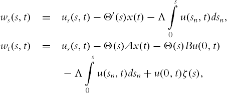
The backstepping transformation
maps the system (4.18)–(4.20) into the target system

This transformation which is defined as ![]() has the lower-triangular form
has the lower-triangular form

Here Γ denotes the operator ![]() , where
, where ![]() is defined as
is defined as

and φ denotes the operator

where Λ is a scalar that will be defined later.
Computing the time and spatial derivatives of the backstepping transformation (4.21) yields
where

Subtracting ![]() gives
gives

Expression (4.25) is an ordinary differential equation. To find its initial condition, we set ![]() in (4.21). Hence
in (4.21). Hence
Introducing (4.27) into (4.22) gives
Comparing this equation with (4.20) implies ![]() . Therefore, the solution of (4.25) is of the form
. Therefore, the solution of (4.25) is of the form
From (4.26), ![]() , where
, where ![]() denotes the inverse operator. Therefore, we have that
denotes the inverse operator. Therefore, we have that
and then ![]() . Substituting the gains Λ and
. Substituting the gains Λ and ![]() into the transformation (4.21) and setting
into the transformation (4.21) and setting ![]() , the controller is then given by
, the controller is then given by
We now prove that the closed-loop system composed of the plant (6.5) and (4.20) with the controller (4.29) is exponentially stable at the origin in the sense of the norm

We first demonstrate that the origin of the target system (4.22) is exponentially stable. Consider the following Lyapunov–Krasovskii functional

where ![]() is the solution of the Lyapunov equation for some
is the solution of the Lyapunov equation for some ![]() and
and ![]() . The time derivative of (4.30) is
. The time derivative of (4.30) is

Let us choose

where ![]() and
and ![]() are the maximum and minimum eigenvalues of the corresponding matrices. It follows that
are the maximum and minimum eigenvalues of the corresponding matrices. It follows that

hence
where

Using the backstepping transformation and its inverse form, we get


Expression (4.30) implies that

where

Furthermore (4.33) and (4.34) give


where

Hence we obtain


where

Notice that the inequalities for ![]() ,
, ![]() for
for ![]() can be combined. Then it follows that
can be combined. Then it follows that

Finally, combining the above with (4.31) gives

where ![]() , which completes the proof of exponential stability.
, which completes the proof of exponential stability.
The predictor algorithm in Theorem 4.2 is obtained for linear systems and delayed linear controllers; however, we will show in the following that it could be applied with delayed nonlinear algorithms forcing its nonlinear dynamics to have a linear behavior, and then guarantee the closed-loop stability. To better illustrate, we apply our approach to a quadcopter vehicle. Aerial vehicles generally move in translational flight (or classical maneuvers) with angles between ±10 grad, which in the aerial control community and for stability analysis is considered as small angles and substantially simplifies the nonlinear equations (2.4)–(2.5) because the Coriolis effects can be neglected given the following equations2:
with Consider now that the control inputs
Remember that θ, ϕ, and ψ represent the pitch, roll, and yaw angles, respectively. In the previous system, it is considered that the control inputs are delayed From (4.40), notice that the yaw angle is a linear system and could be considered decoupled from the others, i.e.,
For the altitude dynamics,
and the closed-loop system is
where
The predicted states for ψ and z have the form
where β is z or ψ.3 The equations for
The previous equations with the roll and pitch dynamics mathematically represent the lateral and longitudinal movements of the quadrotor. These dynamics are the strongest and define the stability of the flying aerial vehicle. Following the ideas proposed in [22], we will prove that nonlinear controllers based on nested saturations can be used with the predictor algorithm to stabilize the quadrotor even in the presence of delayed inputs. It has been also proved in several works that controllers based on saturation functions impose a linear behavior in nonlinear systems when bounding mainly the angular position. Thus in our analysis we will take this fact into account, and it will signify that the quadcopter will move with small angles, i.e., Let us define the linear longitudinal dynamics of the quadrotor as
where Define the observation error as We propose the following control using the predicted states:
where If
Define
Define
Notice that
Define
Take
Observe again that
Finally, define
Take
From Theorem 4.2,
where The predicted states are defined as
where Several simulations are done to validate the proposed predictive-control scheme in the quadrotor model (4.39)–(4.40). Two delays are introduced to test the performance, Simulations were conducted adding and increasing the delays, ( The predictor control scheme is applied with Several experiments are carried out to accomplish the practical goal, i.e., validate the proposed scheme with real-data or in real-time experiments. Here only three cases using different sensors will be presented. First, the predictive algorithm is tested offline and in open-loop with data collected from manual tests. A virtual delay is induced to the data collection, and then the predictive algorithm is applied to the delayed data. Next the resulting array is compared with the original data to verify the performance of the predictive scheme. In the second case, a flight test is realized to follow a square trajectory without any delay in the input. With the collected data virtual delays are induced in all the states to validate the predictive algorithm and verify its behavior with the dynamics of the quadrotor. Finally, for an UAV in a real flight mission, the yaw dynamics (ψ, A rectangular trajectory was made in the manual mode with a LEA-6s GPS sensor, produced by ublox. Collected data were used to test the predictive algorithm offline. The sampling period of the GPS is In Fig. 4.15 the velocity response and a zoom of this figure in the x-axis is presented. Recall that for aerial vehicles the velocity responses need to be very fast in order to stabilize the vehicle. Delaying this state by 1.8 s is not realistic for the sensor characteristics; therefore, it was delayed by only three sampling periods to improve the prediction. Recall also that the sampling period is 200 ms, so the delay for the velocity is 600 ms. Another flight was made to follow a rectangle trajectory in automatic mode without delay. The collected data was delayed in order to apply our predictor control scheme. The height z was imposed to be constant. In the following figures, and due to chapter length limitations, only the position in the horizontal plane is presented (longitudinal and lateral dynamics). First, the delays Multirotor vehicles are the most popular aerial vehicles that can hover. In this part, we propose to validate the predictor–control scheme in a closed-loop system for the yaw dynamics. This test was made with our CoQua (Coaxial-quadrotor) vehicle, or octarotor, shown in Fig. 4.18. The aerial vehicle is controlled with an In this experiment virtual delays are introduced in the yaw dynamics in order to destabilize the yaw dynamics. First, the critical delay value (CDV, delay value capable to destabilize the system) was found using a control scheme without the predictive algorithm. This value was 15 sampling periods, see Fig. 4.19. Notice the unstable ψ response in this figure when applying the delayed controller without predictor, similarly for the The second part consisted of a repeated experiment with the CDV and the predictive algorithm in closed loop. When the predictor is applied to the unstable system, the closed-loop system becomes stable, see Figs. 4.21–4.22. Also in this experiment we added manual changes of reference in order to analyze the system's performance. A zoom of the yaw response can be also appreciated in Fig. 4.21. Fig. 4.22 illustrates the yaw rate response. Notice here that the stability is also recovered for this state. 4.2.1 Aerial Vehicle Validation
4.2.1.1 Mathematical Representation of a Quadrotor with Delayed Inputs
![]() and
and ![]() respectively defining the position and orientation of the vehicle. It is well known that variable τ denotes the delay in the control community. Thus, to avoid confusion in this chapter, the torques
respectively defining the position and orientation of the vehicle. It is well known that variable τ denotes the delay in the control community. Thus, to avoid confusion in this chapter, the torques ![]() will be represented as
will be represented as ![]() , respectively.
, respectively.![]() are delayed, then functions
are delayed, then functions ![]() ,
, ![]() can be defined as
can be defined as![]() sampling periods.
sampling periods.4.2.1.2 Altitude and Yaw Control
![]() . Therefore, applying Theorem 4.2, it follows that
. Therefore, applying Theorem 4.2, it follows that![]() , the following controller is given by
, the following controller is given by![]() is the virtual delayed input and
is the virtual delayed input and ![]() represents the error in the prediction. Hence, if the pair
represents the error in the prediction. Hence, if the pair ![]() , then
, then ![]() . However, applying the predictor–control scheme to (4.42), it follows that
. However, applying the predictor–control scheme to (4.42), it follows that![]() and
and ![]() will be defined later. Introducing (4.41) into (4.39), we have
will be defined later. Introducing (4.41) into (4.39), we have4.2.1.3 Modified Nested Saturation Algorithm for Translational Movements
![]() and
and ![]() . This implies that the lateral and longitudinal dynamics can be represented by four integrators in cascade. In the following, the procedure to fully obtain the controller for the longitudinal dynamics is described step by step, a similar procedure is used to acquire the controller for the lateral dynamics.
. This implies that the lateral and longitudinal dynamics can be represented by four integrators in cascade. In the following, the procedure to fully obtain the controller for the longitudinal dynamics is described step by step, a similar procedure is used to acquire the controller for the lateral dynamics.![]() and
and ![]() is the delayed input.
is the delayed input.![]() . Observe from Theorem 4.1 that if
. Observe from Theorem 4.1 that if ![]() , then
, then ![]() . Thus we can consider that after a time
. Thus we can consider that after a time ![]() ,
, ![]() , so that
, so that ![]() with
with ![]() .
.![]() is a saturation function such that
is a saturation function such that ![]() and
and ![]() is a bounded function,
is a bounded function, ![]() , that will be defined later to prove convergence. We propose the following positive definite function
, that will be defined later to prove convergence. We propose the following positive definite function ![]() , then
, then ![]() .
.![]() then
then ![]() , and if
, and if ![]() , this implies that
, this implies that ![]() . Then after a time
. Then after a time ![]() ,
, ![]() . If we choose
. If we choose ![]() , then
, then ![]()
![]() , then
, then![]() , then
, then ![]() . We propose
. We propose ![]() , then
, then![]() is arbitrarily small and
is arbitrarily small and ![]() , thus, if
, thus, if ![]() , this implies that
, this implies that ![]() and then after a time
and then after a time ![]() ,
, ![]() . If we choose
. If we choose ![]() , then
, then ![]()
![]() , then
, then![]() , then
, then ![]() . Propose
. Propose ![]() , then
, then ![]() . Notice that
. Notice that ![]() and this implies that
and this implies that ![]() is bounded and decreases, so after a time
is bounded and decreases, so after a time ![]() the controller can be rewritten as
the controller can be rewritten as![]() could be expressed as
could be expressed as ![]() , and, in addition, remembering that
, and, in addition, remembering that ![]() , this implies that
, this implies that ![]() . Hence the previous controller becomes
. Hence the previous controller becomes![]() and
and ![]() . The convergence of the states is proved by applying Theorem 4.2.
. The convergence of the states is proved by applying Theorem 4.2.![]() stands for θ and ϕ while
stands for θ and ϕ while ![]() denotes x or y.
denotes x or y.4.2.2 Simulation Results
![]() for the translational motion (x, y, z) and
for the translational motion (x, y, z) and ![]() for the attitude (ψ, θ, ϕ). The sampling period,
for the attitude (ψ, θ, ϕ). The sampling period, ![]() , used in simulation is
, used in simulation is ![]() , the desired values are
, the desired values are ![]() ,
, ![]() , and
, and ![]() , and the initial conditions for all states are set to zero except for
, and the initial conditions for all states are set to zero except for ![]() . First, simulations are made to illustrate good performance of the closed-loop system (4.39)–(4.40) with the control inputs without considering the delays (
. First, simulations are made to illustrate good performance of the closed-loop system (4.39)–(4.40) with the control inputs without considering the delays (![]() ), see Fig. 4.10. For clarity, only the positions (x, y, z) are depicted in this figure.
), see Fig. 4.10. For clarity, only the positions (x, y, z) are depicted in this figure.
![]() ), until instability is presented. The Critical Delay Values (CDV) that induce system instability are
), until instability is presented. The Critical Delay Values (CDV) that induce system instability are ![]() and
and ![]() . The critical values are increased until divergence in the states is observed. Two graphs are presented here to illustrate the performance. On the one hand, Fig. 4.11 depicts the behavior for the position with
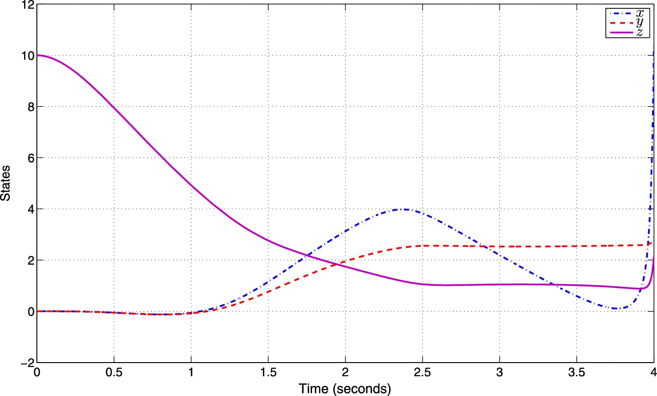
. The critical values are increased until divergence in the states is observed. Two graphs are presented here to illustrate the performance. On the one hand, Fig. 4.11 depicts the behavior for the position with ![]() , here the x position diverges at time
, here the x position diverges at time ![]() . On the other hand, in Fig. 4.12
. On the other hand, in Fig. 4.12 ![]() is increased to
is increased to ![]() , and the system diverges in just 4 seconds.
, and the system diverges in just 4 seconds.
![]() and
and ![]() , and the closed-loop system is restored. Nevertheless, we continue to increase these delays to observe the robustness of the predictor. The critical values were again increasing until
, and the closed-loop system is restored. Nevertheless, we continue to increase these delays to observe the robustness of the predictor. The critical values were again increasing until ![]() and
and ![]() ; the behavior when applying these delays and the PC-S is shown in Fig. 4.13. Observe here that all the states converge to the desired values even though the delays are bigger than the CDV.
; the behavior when applying these delays and the PC-S is shown in Fig. 4.13. Observe here that all the states converge to the desired values even though the delays are bigger than the CDV.
4.2.3 Experimental Results
![]() ) was virtually delayed until signs of instability appeared, then the predictor control scheme is used in closed-loop to compensate the delay.
) was virtually delayed until signs of instability appeared, then the predictor control scheme is used in closed-loop to compensate the delay.Open-Loop with GPS Measurements
![]() . The position data is virtually delayed by
. The position data is virtually delayed by ![]() while the velocity data is delayed by just
while the velocity data is delayed by just ![]() . Figs. 4.14–4.15 show the obtained results and illustrate the delayed measure (red dotted line), the actual state (blue solid line), and the predicted state (black dashed line). Data are depicted in the coordinate system ECEF, and for the length of the chapter only results in the x-axis are presented. In Fig. 4.14 the x-displacement is presented, and to better illustrate the result a zoom of this figure is also shown.
. Figs. 4.14–4.15 show the obtained results and illustrate the delayed measure (red dotted line), the actual state (blue solid line), and the predicted state (black dashed line). Data are depicted in the coordinate system ECEF, and for the length of the chapter only results in the x-axis are presented. In Fig. 4.14 the x-displacement is presented, and to better illustrate the result a zoom of this figure is also shown.

Open-Loop with OptiTrack Measures
![]() and
and ![]() were set to
were set to ![]() . The predictor responses show that the real and predicted values of the states are similar and their difference is almost zero, see Fig. 4.16. Next delays
. The predictor responses show that the real and predicted values of the states are similar and their difference is almost zero, see Fig. 4.16. Next delays ![]() and
and ![]() were increased to
were increased to ![]() . The horizontal position responses are illustrated in Fig. 4.17. Notice that even when the delay is big, the predictor scheme is able to correctly predict the values of the states. From the obtained result, we carried on real-time experiments to implement the predictor algorithm in the closed-loop system of an octarotor vehicle.
. The horizontal position responses are illustrated in Fig. 4.17. Notice that even when the delay is big, the predictor scheme is able to correctly predict the values of the states. From the obtained result, we carried on real-time experiments to implement the predictor algorithm in the closed-loop system of an octarotor vehicle.
 plane trajectory with delays d1 = d2 = 15Ts.
plane trajectory with delays d1 = d2 = 40Ts.4.2.3.1 CoQua Vehicle
![]() that controls eight drivers
that controls eight drivers ![]() , and consequently, the eight motors
, and consequently, the eight motors ![]() which gives the thrust and torques of the vehicle. To measure the attitude (ψ, θ, ϕ), an inertial measurement unit model
which gives the thrust and torques of the vehicle. To measure the attitude (ψ, θ, ϕ), an inertial measurement unit model ![]() of the Microstrain brand is used. The weight of this UAV is 1.6 kg.
of the Microstrain brand is used. The weight of this UAV is 1.6 kg.
![]() state illustrated in Fig. 4.20.
state illustrated in Fig. 4.20.

 response with a delayed input of 15Ts.

response with the predictor control scheme with the delay of 15Ts.


4.3 Discussion
Improving system's behavior is a challenge to many researchers. Several teams work directly on proposing robust controllers that can reject uncertainties, perturbations, or sometimes delays. In this chapter two predictor schemes to improve the closed-loop behavior in the presence of delays in the inputs were proposed. The algorithms considered real cases as delayed measurements on sensors, and it was proved that using these predictors the states are recovered.
The first scheme was based on an Observer–Predictor Algorithm that compensates delays in the control inputs. The algorithm includes an h-step ahead predictor to estimate the delayed state. Simulation and experimental results have demonstrated good performance of the closed loop even when it had been degraded. The second algorithm used the Fundamental Theorem of Calculus to design a predictor scheme to compensate the delays in the system (sensors, etc.). Stability analysis was proved using the ideas in [21]. Simulation and experimental results have corroborated good performance of the algorithm.