
Sliding Mode Control*
Abstract
The sliding controllers are becoming popular when working with aerial vehicles. They are generally used for their good performance and robustness properties in the presence of unknown perturbations. They are often used in nonlinear systems despite their greatest weakness to produce chattering in the control inputs. In this chapter two results are presented: on the one hand, a methodology is described to represent the nonlinear and perturbed attitude dynamics of a quadcopter in a linear and perturbed attitude system as mostly used in several works, and, on the other hand, a robust sliding mode algorithm with an integral component is conceived and validated to stabilize this system. Graphs obtained from simulation and experimental results introduce good performance of the closed-loop system even in the presence of several disturbances and noise in the states.
Keywords
Sliding mode control; Nonlinear MIMO system; Attitude dynamics; Quadcopter vehicle; Real-time validation
Controlling the attitude dynamics of a drone is an essential task when working with aerial vehicles. This dynamics has a nonlinear nature included in the Coriolis matrix, see Chap. 2. It was demonstrated in previous chapters that generally this dynamics is used to conceive control algorithms in its linear or simplified nonlinear mode. Nevertheless, it is also possible to represent these nonlinear equations as linear and perturbed equations, implying the design of controllers in an easy way. Nonlinear controllers are becoming popular when working with UAVs because they can be robust with respect to unknown perturbations such as wind present in the environment. Several researchers have proposed countless algorithms to stabilize the attitude of the aerial vehicle. The sliding mode approach becomes an essential tool due to its robustness and quick dynamics to converge the states. This methodology has been extensively studied in many works, see [1–5].
In this chapter the sliding mode and singular optimal control methodologies are used to design nonlinear controllers to stabilize the nonlinear attitude of a quadcopter vehicle. Two results are introduced here: first, a new form to represent the nonlinear equations for the orientation of a VTOL1 vehicle in the presence of unknown disturbances as a linear MIMO and perturbed system is presented, and second, a control law is proposed and validated in simulations and in real time to stabilize the attitude of a quadcopter.
7.1 From the Nonlinear Attitude Representation to Linear MIMO Expression
The simplest form to represent the orientation of a quadcopter or VTOL vehicle is to consider two integrators in cascade with external perturbations as follows:
¨η=uη+wη,
or
˙x=ˉAx+ˉB1uη+ˉB2wηwithx=[η1η2],
where η represents the attitude vector with η being ϕ, θ, or ψ, i.e., the Euler angles, roll, pitch, and yaw, respectively, uη![]() defines the control input, and wη
defines the control input, and wη![]() the unknown and external perturbation. Even if this representation is experimentally valid for small angles, it does not represent the Coriolis and aerodynamic effects that the aerial vehicle experiences and can generate undesirable dynamics in flight when the vehicle moves quickly.
the unknown and external perturbation. Even if this representation is experimentally valid for small angles, it does not represent the Coriolis and aerodynamic effects that the aerial vehicle experiences and can generate undesirable dynamics in flight when the vehicle moves quickly.
Studying the complete nonlinear attitude equations to design the controller can be an arduous task; nevertheless, some authors prefer to consider the strongest terms in the orientation to represent their model. These equations are described in the following and, considering our experience with quadcopters, they closely represent the attitude of a quadrotor vehicle:
¨ϕ=˙θ˙ψ(Iy−IzIx)−IrIx˙θΩ+lIxuϕ+wϕ,¨θ=˙ϕ˙ψ(Iz−IxIy)−IrIy˙ϕΩ+lIyuθ+wθ,¨ψ=˙θ˙ϕ(Ix−IyIz)+lIzuψ+wψ,

where the distance from each motor to the gravity center of the vehicle is denoted by l. The inertia of the vehicle in each axis is defined by Ix![]() , Iy
, Iy![]() , and Iz
, and Iz![]() while the inertia of the motor is represented by Ir
while the inertia of the motor is represented by Ir![]() , and the speed of the rotor is defined by Ω.
, and the speed of the rotor is defined by Ω.
Notice that system (7.3) is quite different from (7.1) even if the unknown disturbances or uncertainties, wη![]() , are also considered in the model. We study the system with bounded perturbations because it is obvious that the physical characteristics of the vehicle (power motors, etc.) are not unlimited, and, as a consequence, the perturbations need to be bounded, i.e., |wη|≦Lη
, are also considered in the model. We study the system with bounded perturbations because it is obvious that the physical characteristics of the vehicle (power motors, etc.) are not unlimited, and, as a consequence, the perturbations need to be bounded, i.e., |wη|≦Lη![]() , where Lη
, where Lη![]() is a constant that defines the amplitude of each perturbation.
is a constant that defines the amplitude of each perturbation.
Theorem 7.1
System (7.3) is equivalent to system
˙x=Ax+B(u+ˉw)
with x=(ϕ1θ1ψ1ϕ2θ2ψ2)T![]() , u=(uϕuθuψ)T
, u=(uϕuθuψ)T![]() ,
,
ˉw=(θ2(ψ2(Iy−IzIx)−IrIxΩ)−ϕ2+wϕlIxϕ2(ψ2(Iz−IxIy)−IrIyΩ)−θ2+wθlIyθ2ϕ2(Ix−IyIz)−ψ2+wψlIz),A=(03×303×3I3×3I3×3),B=(03×3B2),B2=(lIx000lIy000lIz).

Proof
Consider γ1=(Iy−IzIx)![]() , γ2=(Iz−IxIy)
, γ2=(Iz−IxIy)![]() , γ3=(Ix−IyIz)
, γ3=(Ix−IyIz)![]() , β1=IrIxΩ
, β1=IrIxΩ![]() , β2=IrIyΩ
, β2=IrIyΩ![]() , b1=lIx
, b1=lIx![]() , b2=lIy
, b2=lIy![]() , and b3=lIz
, and b3=lIz![]() . Define ϕ1=ϕ
. Define ϕ1=ϕ![]() , θ1=θ
, θ1=θ![]() , ψ1=ψ
, ψ1=ψ![]() , ˙ϕ1=ϕ2
, ˙ϕ1=ϕ2![]() , ˙θ1=θ2
, ˙θ1=θ2![]() , and ˙ψ1=ψ2
, and ˙ψ1=ψ2![]() .
.
Then, rewriting (7.3) it follows that
˙ϕ1=ϕ2,˙ϕ2=θ2(ψ2γ1−β1)+b1uϕ+wϕ,˙θ1=θ2,˙θ2=ϕ2(ψ2γ2−β2)+b2uθ+wθ,˙ψ1=ψ2,˙ψ2=θ2ϕ2γ3+b3uψ+wψ.

To simplify the analysis, define f1=θ2(ψ2γ1−β1)![]() , f2=ϕ2(ψ2γ2−β2)
, f2=ϕ2(ψ2γ2−β2)![]() , and f3=θ2ϕ2γ3
, and f3=θ2ϕ2γ3![]() . Taking the three right equations of (7.5), we obtain
. Taking the three right equations of (7.5), we obtain
˙ϕ2=ϕ2−ϕ2+f1+b1uϕ+wϕ,˙θ2=θ2−θ2+f2+b2uθ+wθ,˙ψ2=ψ2−ψ2+f3+b3uψ+wψ.

Define Φ1=f1−ϕ2![]() , Φ2=f2−θ2
, Φ2=f2−θ2![]() , and Φ3=f3−ψ2
, and Φ3=f3−ψ2![]() . Then
. Then
˙ϕ2=ϕ2+b1(uϕ+ˉwϕ),˙θ2=θ2+b2(uθ+ˉwθ),˙ψ2=ψ2+b3(uψ+ˉwψ)
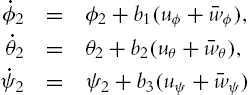
with ˉwi=(Φi+wη)/bi![]() . Finally, define ηi=(ϕiθiψi)T
. Finally, define ηi=(ϕiθiψi)T![]() , i=1,2
, i=1,2![]() . Then we can write
. Then we can write
˙η1=η2,˙η2=η2+B2(u+ˉw),

which is equivalent to system (7.4).
7.2 Nonlinear Optimal Controller with Integral Sliding Mode Design
The goal is to stabilize the quadcopter attitude using an optimal control u that is robust with respect to perturbations and parameter variations. For this it is necessary to minimize the following singular quadratic cost:
J(x(t))=12∞∫t1[x(t)TQx(t)]dt,

with Q=QT>0![]() . The minimization of (7.6) is subject to
. The minimization of (7.6) is subject to
˙η1=η2.
Developing (7.6), it follows that
J=12∞∫t1(η1TQ11η1+2η1TQ12η2+η2TQ22η2)dt.

To eliminate the cross terms, the Utkin variable υ=η2+Q−122QT12η1![]() is used. Then
is used. Then
J=12∞∫t1(ηT1Q1η1+υTQ22υ)dt

with Q1=Q11−Q12Q−122QT12![]() . Rewriting (7.7) with the Utkin variable yields
. Rewriting (7.7) with the Utkin variable yields
˙η1=A1η1+υ,
where A1=−Q−122QT12![]() . Then (7.9) is not singular with respect to the variable υ, so that υ is taken as an optimal virtual control variable and is given by
. Then (7.9) is not singular with respect to the variable υ, so that υ is taken as an optimal virtual control variable and is given by
υ=−Q−122Pη1,
where P∈R3×3![]() is the solution to the Riccati equation PA1+AT1P−PQ−122P+Q1=0
is the solution to the Riccati equation PA1+AT1P−PQ−122P+Q1=0![]() . Introducing the Utkin variable into (7.11), we have
. Introducing the Utkin variable into (7.11), we have
η2+Q−122(QT12+P)η1=0.
Notice that (7.11) and (7.12) are only true if (7.9) is minimized for all t1⩾0![]() .
.
Observe that (7.12) is an optimal vector that can be used for designing the vector S∈R3![]() given by
given by
S=η2+Q−122(QT12+P)η1,
where (7.13) represents the sliding surface vector. Taking the derivative of the previous equation with respect to time gives
˙S=[I3×3+Q−122(QT12+P)]η2+B2(u+ˉw).
To remove the linear parts, take u as
u=B−12{ˉu−[I3×3+Q−122(QT12+P)]η2}.
Thus
˙S=ˉu+B2w,
where ˉu![]() is the new controller to assure the convergence of the system. Developing the above, it follows that
is the new controller to assure the convergence of the system. Developing the above, it follows that
(˙S1˙S2˙S3)=(ˉu1+f1−ϕ2+wϕˉu2+f2−θ2+wθˉu3+f3−ψ2+wψ).

To remove the linearities η2![]() , we propose ˉu
, we propose ˉu![]() as
as
ˉu=(ˉu1ˉu2ˉu3)=(ˉv1+ϕ2ˉv2+θ2ˉv3+ψ2).

Then, rewrite ˙S![]() as
as
˙S=(ˉv1+f1+wϕˉv2+f2+wθˉv3+f3+wψ),

where each ˙Si∈˙S![]() is represented as
is represented as
˙Si=ˉvi+fi(η1,η2,t)+wη.
7.2.1 Convergence of the Sliding Surfaces
In the conventional sliding mode control the robustness property is not guaranteed from the first time instant because the robustness is only guaranteed when the sliding surface reaches zero.
With the integral sliding mode we will be able to compensate nonlinear terms and bounded uncertainties, also the robustness will be guaranteed from the initial time instance. In the following, we introduce variable ˉvi![]() to stabilize the sliding surfaces.
to stabilize the sliding surfaces.
Then, we propose
ˉvi=ˉvi1+ˉvi2.
• Part ˉvi1![]() will be responsible of compensating the nonlinear terms fi
will be responsible of compensating the nonlinear terms fi![]() and the bounded disturbance wη
and the bounded disturbance wη![]() from the beginning.
from the beginning.
• Component ˉvi2![]() will make sure that each sliding surface Si
will make sure that each sliding surface Si![]() reaches the optimal surface Si=0
reaches the optimal surface Si=0![]() at a defined finite time t1
at a defined finite time t1![]() taking in consideration that the perturbations fi
taking in consideration that the perturbations fi![]() and wη
and wη![]() have been compensated from the initial time instance t=0
have been compensated from the initial time instance t=0![]() .
.
For ˉvi1
{σi=Si−Zi,˙Zi=ˉvi2.
It should be mentioned that ˉvi1
V(σi)=12σ2i>0.
The asymptotic stability of (7.19) at the equilibrium point 0 can be proved if the following conditions are satisfied:
(a)lim|σi|→∞V=∞,
(b)˙V<0for σi≠0.
Condition (a) is obviously satisfied by V in (7.20). Nevertheless, the finite-time convergence (global finite-time stability) could be achieved if condition (b) is modified as
˙V⩽−αiV1/2,αi>0.
Indeed, separating variables and integrating inequality (7.23) over the time interval 0⩽τ⩽t
V1/2(σi(t))⩽−12αit+V1/2(σi(0)),
and, considering that V(σi(t))
tr⩽2V1/2(σi(0))αi.
Therefore control ˉvi1 Now notice that (7.23) can be written as
σi˙σi⩽−ˉαi|σi|,ˉαi=αi√2,ˉαi>0.
Consequently, from the above and with (7.17), (7.18) and (7.19) we have
σi⁎(˙Si−˙Zi)=σi⁎(ˉvi1+ˉvi2+fi(η1,η2,t)+wη−ˉvi2)=σi⁎(ˉvi1+fi(η1,η2,t)+wη),
and, selecting ˉvi1=−ρisgn(σi)
ρi=ˉαi+|fi(η1,η2,t)|+Lη.
Notice that (7.27) represents the necessary gains for ensuring the finite time stability in a bounded finite time tr
tr⩽2V1/2(σi(0))αi=|σi(0)|ˉα.
The above implies that σi=˙σi=0
˙σi=−ρisgn(σi)︸ˉvi1+fi(η1,η2,t)+wη=0∀t⩾tr,
meaning that −ρ1sgn(σi) In the following, to eliminate the reaching phase, we observe in (7.28) that proposing σi(0)=0 Based on the above considerations, we present the next result
ˉvi1=−ρisgn(σi)=−(fi(η1,η2,t)+wη),∀t⩾0
if and only if σi(0)=0 Therefore control ˉvi1=−ρisgn(σi) Now considering that control ˉvi1
{Si=Zi,˙Zi=ˉvi2,with Zi(0)=Si(0).
Then considering (7.29) we have
˙Si=ˉvi2.
The next step is to design ˉvi2 In order to achieve global finite-time stability at the optimal sliding surfaces Si=0
˙Si=−ki|Si|1/2sgn(Si).
The following Lyapunov function is proposed to prove that (7.30) converges to zero in finite time:
V(Si)=|Si|>0.
The previous equations must satisfy conditions (7.22). Observe that, by definition (7.31), condition (a) is achieved; to fulfill condition (b), we use (7.23). Notice that when introducing (7.31) into (7.23) an equivalent modified condition is obtained, which is given by
Si˙Si|Si|⩽−αi|Si|1/2.
Introducing (7.30) into (7.32), the previous inequality becomes
−ki|Si|1/2⩽−αi|Si|1/2.
Therefore to satisfy (7.33) each gain ki
˙V=−αiV1/2ifki=αi>0.
Observe that the finite-time convergence time tri
tri=2V1/2(Si(0))ki=2|Si(0)|1/2ki;
consequently, Si=0 Fixing tri=t1=cte Summarizing the methodology, it follows that when considering (7.17) and the fact that ˉvi=ˉvi1+ˉvi2
˙Si=−ρisgn(Si−Zi)︸ˉvi1+(−ki|Si|1/2sgn(Si))︸ˉvi2+fi+wη
with gains
ρi=ˉαi+|fi(η1,η2,t)|+Lηandki=2|Si(0)|1/2t1.
• Component ˉvi1 • Considering that the perturbative terms have been compensated from the initial time, control ˉvi2
Therefore, component ˉui
ˉui=−ρisgn(Si−Zi)−ki|Si|1/2sgn(Si)+η2i,Zi=−ki∫|Si|1/2sgn(Si)dtwith Zi(0)=Si(0),
and gains t1=cteDesign of ˉvi1
![]()
![]() we propose a new auxiliary surface σi
we propose a new auxiliary surface σi![]() with i=1,2,3
with i=1,2,3![]() given by2
given by2![]() is designed as a conventional sliding mode control. This means that for the stability analysis a candidate Lyapunov function could be used. Therefore
is designed as a conventional sliding mode control. This means that for the stability analysis a candidate Lyapunov function could be used. Therefore![]() , we obtain
, we obtain![]() reaches zero in finite time tr
reaches zero in finite time tr![]() , get
, get![]() that satisfies (7.23) will drive σi
that satisfies (7.23) will drive σi![]() to zero in finite time tr
to zero in finite time tr![]() and will keep it at zero ∀t⩾tr
and will keep it at zero ∀t⩾tr![]() .
.![]() , condition (7.26) is fulfilled if and only if
, condition (7.26) is fulfilled if and only if![]() , which means
, which means![]() for all t⩾tr
for all t⩾tr![]() , then the condition ˙σi=0
, then the condition ˙σi=0![]() produces
produces![]() will compensate the perturbative terms fi(η1,η2,t)+wη
will compensate the perturbative terms fi(η1,η2,t)+wη![]() only during the reaching phase.
only during the reaching phase.![]() will imply tr=0
will imply tr=0![]() and as a result σi=˙σi=0
and as a result σi=˙σi=0![]() for all t⩾0
for all t⩾0![]() .
. ![]() .
.![]() compensates fi(η1,η2,t)+wη
compensates fi(η1,η2,t)+wη![]() for all t⩾0
for all t⩾0![]() if and only if σi(0)=0
if and only if σi(0)=0![]() .
.![]() accomplishes σi(t)=0
accomplishes σi(t)=0![]() for all t⩾0
for all t⩾0![]() and due to (7.19), it follows that Si(t)=Zi(t)
and due to (7.19), it follows that Si(t)=Zi(t)![]() for all t⩾0
for all t⩾0![]() . Therefore (7.19) can be rewritten as
. Therefore (7.19) can be rewritten as![]() such that Si
such that Si![]() converges to zero in finite time.
converges to zero in finite time.Design of ˉvi2
![]()
![]() , we introduce ˉvi2=−ki|Si|1/2sgn(Si)
, we introduce ˉvi2=−ki|Si|1/2sgn(Si)![]() ; then ˙Si
; then ˙Si![]() is written as
is written as![]() must be equal to αi
must be equal to αi![]() , meaning that ki>0
, meaning that ki>0![]() , and this implies that
, and this implies that![]() will not be bounded, it will be exactly equal to
will not be bounded, it will be exactly equal to![]() in a finite time tri
in a finite time tri![]() . Observe that (7.34) represents the finite-time convergence of each Si
. Observe that (7.34) represents the finite-time convergence of each Si![]() to the optimal sliding surface Si=0
to the optimal sliding surface Si=0![]() . With the purpose that each Si
. With the purpose that each Si![]() has the same finite time convergence, we fix tri=t1=cte
has the same finite time convergence, we fix tri=t1=cte![]() ,3 then we will be able to design the gains ki
,3 then we will be able to design the gains ki![]() in order to have S1(t1)=S2(t1)=⋯=Sn(t1)=0
in order to have S1(t1)=S2(t1)=⋯=Sn(t1)=0![]() .
.![]() , the necessary gains for getting Si(t1)=0
, the necessary gains for getting Si(t1)=0![]() can be obtained with ki=2|Si(0)|1/2t1
can be obtained with ki=2|Si(0)|1/2t1![]() .
.![]() , we have
, we have![]() will compensate the perturbative terms fi(η1,η2,t)+wη
will compensate the perturbative terms fi(η1,η2,t)+wη![]() for all t⩾0
for all t⩾0![]() if and only if Zi(0)=Si(0)
if and only if Zi(0)=Si(0)![]() .
.![]() will ensure that every Si
will ensure that every Si![]() will converge to the optimal sliding surface Si=0
will converge to the optimal sliding surface Si=0![]() in a fixed reaching time t1
in a fixed reaching time t1![]() .
.![]() from (7.15) is given by
from (7.15) is given by![]() and ˉαi=αi√2
and ˉαi=αi√2![]() in (7.35).
in (7.35).


7.3 Numerical Validation
Simulations are realized to validate the proposed controllers. From section 7.1 notice that (7.3) can be expressed in regular form as
˙η1=η2,˙η2=η2+B2(u+ˉw),
where η1=(ϕ1,θ1,ψ1)T![]() and η2=(ϕ2,θ2,ψ2)T
and η2=(ϕ2,θ2,ψ2)T![]() .
.
Following the previous control procedure, some matrices are necessary to compute u. These matrices are proposed as follows:
Q=QT=(1787−6−42826644137611912−6492394−4419932132438)>0,

thus
Q11=(178782667611),Q12=QT12=(−6−424413912),Q22=(2394993438).

Therefore, from (7.9) and (7.10),
Q1=(13.19243.92448.03783.92444.57733.71138.03783.71136.1443),

A1=(0.17870.1203−0.56010.4330−0.00340.5017−0.5017−1.6838−0.1581).

Solving the Riccati equation, it follows that
P=(25.31329.9395−0.51819.93958.9679−1.5217−0.5181−1.52174.4597),

and finally S can be written as
S=η2+Q−122(QT12+P)︸Mη1,

where
M=(M11M12M13M21M22M23M31M32M33)=(0.9702−0.00360.5814−0.24041.1036−0.9275−0.20971.02280.8646).

Then, the sliding surfaces are given by
S1=ϕ2+M11ϕ1+M12θ1+M13ψ1,S2=θ2+M21ϕ1+M22θ1+M23ψ1,S3=ψ2+M31ϕ1+M32θ1+M33ψ1.

Rewriting u∈R3![]() , it follows that
, it follows that
uϕ=(Ix/l)(ˉu1−M13ψ2−M12θ2−(M11+1)ϕ2),uθ=(Iy/l)(ˉu2−M21ϕ2−M23ψ2−(M22+1)θ2),uψ=(Iz/l)(ˉu3−M31ϕ2−M32θ2−(M33+1)ψ2),

with
ˉu1=−ρ1sgn(S1−Z1)−k1|S1|1/2sgn(S1)+ϕ2,Z1=−k1∫|S1|1/2sgn(S1)dtwithZ1(0)=S1(0),ˉu2=−ρ2sgn(S2−Z2)−k2|S2|1/2sgn(S2)+θ2,Z2=−k2∫|S2|1/2sgn(S2)dtwithZ2(0)=S2(0),ˉu3=−ρ3sgn(S3−Z3)−k3|S3|1/2sgn(S3)+ψ2,Z3=−k3∫|S3|1/2sgn(S3)dtwithZ3(0)=S3(0),

and gains given by
ρ1=(α1√2+|θ2(ψ2γ1−β1)|+L1),ρ2=(α2√2+|ϕ2(ψ2γ2−β2)|+L2),ρ3=(α3√2+|θ2ϕ2γ3|+L3).

k1=2|S1(0)|1/2t1k2=2|S2(0)|1/2t1k3=2|S3(0)|1/2t1|,t1=cte

The initial conditions were set as ϕ1(0)=−5![]() , θ1(0)=2
, θ1(0)=2![]() , ψ1(0)=−3
, ψ1(0)=−3![]() , all in grad, ϕ2(0)=6
, all in grad, ϕ2(0)=6![]() , θ2(0)=4
, θ2(0)=4![]() , ψ2(0)=6
, ψ2(0)=6![]() in grad/s. These conditions imply S1(0)=−0.6026
in grad/s. These conditions imply S1(0)=−0.6026![]() , S2(0)=10.1917
, S2(0)=10.1917![]() , and S3(0)=6.5004
, and S3(0)=6.5004![]() . We can also define t1=1 s
. We can also define t1=1 s![]() as a finite-time convergence instance for the sliding surfaces S1
as a finite-time convergence instance for the sliding surfaces S1![]() , S2
, S2![]() , and S3
, and S3![]() . Thus, from (7.38) we obtained k1=1.5525
. Thus, from (7.38) we obtained k1=1.5525![]() , k2=6.3849
, k2=6.3849![]() , and k3=5.0992
, and k3=5.0992![]() . Furthermore, for simulation purposes we assumed α1=0.12
. Furthermore, for simulation purposes we assumed α1=0.12![]() , α2=0.14
, α2=0.14![]() , and α3=0.2
, and α3=0.2![]() . The bounded disturbances were selected as follows:
. The bounded disturbances were selected as follows:
wϕ=2sin(t)sgn(S1),|wϕ|≦Lϕ=2,wθ=−1.5cos(2t)sgn(S2),|wθ|≦Lθ=1.5,wψ=−0.5exp(cos(t))sgn(S3),|wψ|≦Lψ=0.5exp(1).

The above disturbances were considered multiplied by sgn(Si)![]() for the following reasons:
for the following reasons:
1. To observe that the effect chattering produced by sgn(Si)![]() is not relevant for the compensation of such disturbances. We are only interested in the knowledge of the maximum amplitude that each perturbation can reach, and not in the high frequency that it can produce.
is not relevant for the compensation of such disturbances. We are only interested in the knowledge of the maximum amplitude that each perturbation can reach, and not in the high frequency that it can produce.
2. To graphically validate the theory. It is expected to observe an evident chattering effect in wϕ![]() , wθ
, wθ![]() , and wψ
, and wψ![]() when Si=0
when Si=0![]() at the desired finite time t1=1
at the desired finite time t1=1![]() .
.
The following graphs were obtained when applying the proposed control scheme. From Fig. 7.1 observe that the auxiliary sliding surfaces σ1![]() , σ2
, σ2![]() , and σ3
, and σ3![]() are zero from the initial time instance, meaning that the robustness is guaranteed with respect to bounded uncertainties all the time. Besides, S1
are zero from the initial time instance, meaning that the robustness is guaranteed with respect to bounded uncertainties all the time. Besides, S1![]() , S2
, S2![]() , and S3
, and S3![]() converge to zero in a desired finite time t1=1
converge to zero in a desired finite time t1=1![]() ; this means that the vector of sliding surface S=η2+Q−122(QT12+P)η1
; this means that the vector of sliding surface S=η2+Q−122(QT12+P)η1![]() converges to the optimal vector of sliding surfaces S=0
converges to the optimal vector of sliding surfaces S=0![]() in finite time t1=1
in finite time t1=1![]() , and with this fact every solution η1=(ϕ,θ,ψ)T
, and with this fact every solution η1=(ϕ,θ,ψ)T![]() and η2=(˙ϕ,˙θ,˙ψ)T
and η2=(˙ϕ,˙θ,˙ψ)T![]() that belongs to S=0
that belongs to S=0![]() will be called an optimal sliding mode because it will be able to minimize the cost function (7.9) for all t⩾t1
will be called an optimal sliding mode because it will be able to minimize the cost function (7.9) for all t⩾t1![]() and in this manner solve the LQR problem.4
and in this manner solve the LQR problem.4

In Fig. 7.2 an asymptotic stabilization is clearly visible for the dynamics of ϕ,θ,ψ![]() and ˙ϕ,˙θ,˙ψ
and ˙ϕ,˙θ,˙ψ![]() due to the convergence of the vector S to the optimal sliding vector S=0
due to the convergence of the vector S to the optimal sliding vector S=0![]() in finite time t1=1
in finite time t1=1![]() .
.

 , ˙θ
, ˙θ , ˙ψ
, ˙ψ .
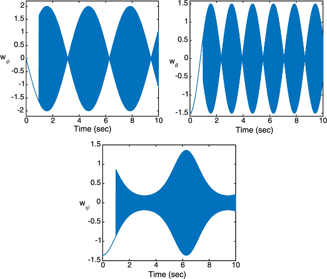
.In Fig. 7.3 it can be observed that the bounded uncertainties wϕ![]() , wθ
, wθ![]() , and wψ
, and wψ![]() present an evident chattering effect by considering the factor sgn(Si)
present an evident chattering effect by considering the factor sgn(Si)![]() , and also that this chattering effect appears at time t1=1
, and also that this chattering effect appears at time t1=1![]() . However, although these uncertainties present a high frequency, the control signal responses uϕ
. However, although these uncertainties present a high frequency, the control signal responses uϕ![]() , uθ
, uθ![]() , and uψ
, and uψ![]() shown in Fig. 7.4 compensate such perturbations from the initial time instance t=0
shown in Fig. 7.4 compensate such perturbations from the initial time instance t=0![]() .
.

In Fig. 7.4 it is shown that the control signal responses uϕ![]() , uθ
, uθ![]() , and uψ
, and uψ![]() have a chattering effect from the beginning, meaning that such controllers are compensating the proposed bounded uncertainties wϕ
have a chattering effect from the beginning, meaning that such controllers are compensating the proposed bounded uncertainties wϕ![]() , wθ
, wθ![]() , and wψ
, and wψ![]() for all t⩾0
for all t⩾0![]() .
.
7.3.1 Emulation Results
One of the problems existing today is due to the discontinuity produced by the sgn function. This discontinuity produces a high frequency, normally called the chattering effect, which in practical applications is not convenient because it could produce unwanted vibrations that could damage the instruments in real-time implementations. Nevertheless, there exists extensive literature on techniques that help diminish the chattering effect.
Notice the chattering effect produced by the sgn function in Fig. 7.4. If we want to improve the performance of the control inputs, several tricks could be used. One technique used frequently is to approximate the sgn function; see, for example, [6, Chap. 1]. This approximation can be applied as
sgn(σ)≈σ|σ|+ϵ.
For our simulations purposes we consider ϵ=0.0007![]() .
.
The idea when validating the proposed algorithm is to have similar results in simulations and/or experiments. For this we consider that all states ϕ, θ, ψ, ˙ϕ![]() , ˙θ
, ˙θ![]() , and ˙ψ
, and ˙ψ![]() are affected by some kind of white noise (that it is true when using inertial sensors). Under these assumptions the following graphs are obtained.
are affected by some kind of white noise (that it is true when using inertial sensors). Under these assumptions the following graphs are obtained.
In Fig. 7.5 we observe that the sliding surfaces S1![]() , S2
, S2![]() , and S3
, and S3![]() converge to zero in finite time t1
converge to zero in finite time t1![]() , although the nonlinear system is being affected by white noise. In Fig. 7.6 asymptotic convergence is observed for the dynamics of ϕ,θ,ψ
, although the nonlinear system is being affected by white noise. In Fig. 7.6 asymptotic convergence is observed for the dynamics of ϕ,θ,ψ![]() and ˙ϕ,˙θ,˙ψ
and ˙ϕ,˙θ,˙ψ![]() in spite of having white noise in the internal dynamics of the system. Due to this, the controls shown in Fig. 7.7 achieve the convergence of the vector S to the optimal sliding vector S=0
in spite of having white noise in the internal dynamics of the system. Due to this, the controls shown in Fig. 7.7 achieve the convergence of the vector S to the optimal sliding vector S=0![]() in finite time. In Fig. 7.7 a representation of the controllers uϕ
in finite time. In Fig. 7.7 a representation of the controllers uϕ![]() , uθ
, uθ![]() , and uψ
, and uψ![]() is shown; they drive S to zero in finite time in the presence of white noise and bounded uncertainties.
is shown; they drive S to zero in finite time in the presence of white noise and bounded uncertainties.

 , ˙θ, ˙ψ with sensor noise.
7.4 Real-Time Validation
The previous controller was validated on our platform (see Sect. 4.1.5 of Chap. 4) to analyze the attitude performance of a quadcopter. Manual and aggressive references were given to test the behavior of the controller. The following main graphs illustrate the results.
Applying the controller as obtained in Sect. 7.3 in real time is very difficult, and the system is very sensible to small changes. This effect appears because even if the sliding surfaces go to zero, the cross terms of other variables are present in these surfaces, e.g., recall that surface S1![]() is for assuring the roll angle convergence and notice that pitch and yaw terms are also included. In addition, if the terms Mij
is for assuring the roll angle convergence and notice that pitch and yaw terms are also included. In addition, if the terms Mij![]() of these variables (pitch and yaw) are bigger then they will strongly influence the controller performance. Therefore, in this part we will include a theoretical–practical tune up that could be used for sliding controllers.
of these variables (pitch and yaw) are bigger then they will strongly influence the controller performance. Therefore, in this part we will include a theoretical–practical tune up that could be used for sliding controllers.
Observe that S=vq+Mq![]() . Then we can choose M not only to assure convergence of the sliding surfaces but also to facilitate the implementation in real time. Therefore the goal will be to weigh the main diagonal of M to assure good convergence of each state. Remember that M is given by M=Q−122(QT12+P)
. Then we can choose M not only to assure convergence of the sliding surfaces but also to facilitate the implementation in real time. Therefore the goal will be to weigh the main diagonal of M to assure good convergence of each state. Remember that M is given by M=Q−122(QT12+P)![]() and Q is given by
and Q is given by
Q=QT=(Q11Q12QT12Q22)>0,Q11,Q12,Q22∈R3×3.

For a practical tune up we can consider Q12=03×3![]() and Q22
and Q22![]() as
as
Q22=(r000s000g)

with r, s, and g being positive numbers to guarantee Q22=QT22>0![]() . Hence M becomes
. Hence M becomes
M=(P11/r000P22/s000P33/g)=(M11000M22000M33),

and this implies that each Si![]() is given by
is given by
S1=ϕ2+M11ϕ1,S2=θ2+M22θ1,S3=ψ2+M33ψ1.

Then u∈R3![]() for practical validation is given as
for practical validation is given as
uϕ=(Ix/l)(ˉu1−(M11+1)ϕ2),uθ=(Iy/l)(ˉu2−(M22+1)θ2),uψ=(Iz/l)(ˉu3−(M33+1)ψ2),

with
ˉu1=−ρ1sgn(S1−Z1)−k1|S1|1/2sgn(S1)+ϕ2,Z1=−k1∫|S1|1/2sgn(S1)dtwithZ1(0)=S1(0),ˉu2=−ρ2sgn(S2−Z2)−k2|S2|1/2sgn(S2)+θ2,Z2=−k2∫|S2|1/2sgn(S2)dtwithZ2(0)=S2(0),ˉu3=−ρ3sgn(S3−Z3)−k3|S3|1/2sgn(S3)+ψ2,Z3=−k3∫|S3|1/2sgn(S3)dtwithZ3(0)=S3(0).

The new gains are given by
ρ1=(α1√2+|θ2(ψ2γ1−β1)|+L1),ρ2=(α2√2+|ϕ2(ψ2γ2−β2)|+L2),ρ3=(α3√2+|θ2ϕ2γ3|+L3),

and other parameters are
k1=2|S1(0)|1/2t1k2=2|S2(0)|1/2t1k3=2|S3(0)|1/2t1|t1=cte,

β1=β2(γ1+1),γ3=−γ1(1γ2(γ1+1)+1),b2=b1(γ1+1),b3=b1[γ2(γ1+1)+1],b−12=(γ1+1)b1,b−13=[γ2(γ1+1)+1]b1.

Analyzing the previous gains, we can observe that the gains for heuristic tune up are β2,γ1,γ2![]() , and b1
, and b1![]() . Thus, the gains can be proposed as
. Thus, the gains can be proposed as
ρ1=(|θ2(ψ2γ1−β1)|+Lx),ρ2=(|ϕ2(ψ2γ2−β2)|+Ly),ρ3=(|θ2ϕ2γ3|+Lz),

and if we want  and
and  then for the tune up we can use the following expressions:
γ3=−γ1γ1+1,γ1,b1=any number,b2=b3=b1(γ1+1),

and then the gains become ρ1=(Lx),ρ2=(Ly)![]() , and ρ3=(|θ2ϕ2γ3|+Lz)
, and ρ3=(|θ2ϕ2γ3|+Lz)![]() .
.
Fig. 7.8 introduces the behavior of the controllers when they are applied in a quadcopter prototype. Observe in this figure that the controller performs well in practice and that the closed-loop system is guaranteed even in the presence of aggressive maneuvers. Also notice that the procedure to tune the gains in the controller works pretty well and can be applied to others sliding controllers. Desired references were given manually by the pilot. Notice that several changes were produced to observe the performance of the controller.

7.5 Discussion
Sliding mode control is becoming a popular tool when working with UAVs since robustness and quick convergence properties make such controllers very interesting to apply in autonomous vehicles. On the negative side, the main problem is the chattering effect produced in the control responses. This effect could damage the physical parts of the system and could require lots of energy for good efficiency. New controllers as proposed in this chapter try to reduce these drawbacks and improve the performance of such algorithms. Nevertheless, many issues still need to be solved and remain an open research topic.
The controller presented in this chapter was designed to be robust with respect to unknown and bounded perturbations and to guarantee convergence in finite time. This fact is not typical in controllers. From emulation results we could observe good performance of the algorithms. The next step for this controller will be to reduce the chattering effect in its design. In addition, a methodology to theoretically tune sliding algorithms was also presented in this chapter. It is very useful when applying the controller in real time. The graphs obtained when implementing the proposed controller demonstrated good performance in closed-loop system.