
Chapter 1: Theoretical basis
Abstract
This chapter gives a brief introduction to artificial intelligence (AI). It starts by reviewing the history of AI. Then it introduces deep learning, which is the recent trend in AI, from its history, applications to future challenges. The last part of the chapter reviews the theory of neural network, which is the basis of deep learning. It introduces the neuron model, perception, multilayer perception, convolutional neural network (CNN), as well as application examples.
Keywords
Artificial intelligence; AI; Deep learning; Neural network; Perception; Convolutional neural network; CNN
1.1: Brief history of artificial intelligence
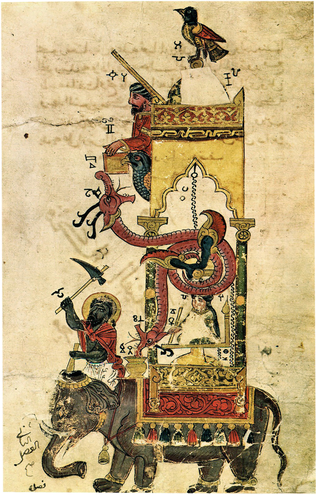
When the development of a skill reaches the peak, it can reflect highly anthropomorphic intelligence. From Ancient China’s Master Yan’s ability to sing and dance, to Ancient Arabic Jazari’s automatic puppets (as shown in Fig. 1.1), the relentless pursuit of intelligence never ends. Human beings hope to give wisdom and thought to machines, which can be used to liberate productive forces, facilitate people’s lives, and promote social development. From ancient myths to science fiction, and now to modern science and technology, they all demonstrate the human desire for intelligence. The birth of artificial intelligence (AI) was a slow and long process, whereas the improvement of AI is keeping pace with the development of human knowledge and even transcending human wisdom in some aspects. In the early days, the development of Formal Reasoning provided a research direction for the mechanization of human intelligence.
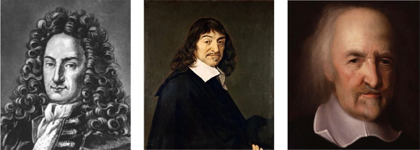
In the mid-17th century, Gottfried Wilhelm Leibniz, Rene Descartes, and Thomas Hobbes (Fig. 1.2) devoted themselves to the systematic study of rational thinking. These studies led to the emergence of the formal symbol system that became the beacon of AI research. By the 20th century, the contributions of Bertrand Arthur William Russell, Alfred North Whitehead, and Kurt Godel in the field of mathematical logic provided a theoretical basis for the mechanization of mathematical reasoning. The creation of the Turing Machine provided supporting evidence of machine thought from the view of semiotics. In the engineering domain, from Charles Babbage’s original idea of “Instrumental Analysis” to the large ENIAC decoding machine serving in World War II, we have witnessed the realization of the theories of Alan Turing and John von Neumann (see Fig. 1.3), which has accelerated the development of AI.

1.1.1: Birth of AI
In the mid-20th century, scientists from different fields made a series of preparations for the birth of AI, including Shannon’s information theory, Turing’s computational theory, and the development of Neurology.
In 1950, Turing published the paper Computing Machinery and Intelligence. In this paper, the famous Turing test was proposed: If a machine can answer any questions to it, using the same words that an ordinary person would, then we may call that machine intelligent. The proposal of the Turing test is of great significance to the development of AI in more recent times. In 1951, the 24-year-old Marvin Minsky, as well as Dean Edmonds, built the Stochastic Neural Analog Reinforcement Calculator. Minsky continued to work in the field of AI, playing a huge role in promoting the development of AI, which contributed to his winning of Turing Award. In 1955, a program called Logic Theorist was introduced and subsequently refined. The ingenious method proved 38 of 52 theorems in the Principles of Mathematics. With this work, the authors Allen Newell and Herbert Simon opened a new methodology for intelligent machines.
A year later, 10 participants at the Dartmouth Conference, including McCarthy, Shannon, and Nathan Rochester, argued that “any aspect of learning or intelligence should be accurately described so that people can build a machine to simulate it.” In that moment, AI entered the world with its mission clearly defined, opening up a brand new world of science.
1.1.2: Set sail
After the Dartmouth Conference, AI developments proceeded akin to a volcanic eruption. The conference started a wave of activity that swept across the globe. Through these developments, significant progress was achieved. Computers were shown to succeed at more advanced tasks, such as solving algebraic problems, geometric proofs, and certain problems in the field of language processing. These advances made researchers enthusiastic and confident about the improvement of AI, and attracted a large amount of funds to the research field.
In 1958, Herbert Gelernter implemented a geometric theorem-roving machine based on a search algorithm. Newell and Simon extended the application of search-based reasoning through a “General Problem Solver” program. At the same time, search-based reasoning was applied to decision-making, such as STRIPS, a Stanford University robotic system. In the field of natural language, Ross Quillian developed the first Semantic Web. Subsequently, Joseph Weizenbaum created the first dialogue robot, ELIZA. ELIZA was sufficiently lifelike that it could be mistaken for a human being when communicating with a person. The advent of ELIZA marked a great milestone in AI. In June 1963, MIT received funding from the United States Agency for Advanced Research Projects (ARPA) to commercialize the MAC (The Project on Mathematics and Computation) project. Minsky and McCarthy were major participants in the project. The MAC project played an important role in the history of AI and also in the development of computer science, giving birth to the famous MIT Computer Science and Artificial Intelligence Laboratory.
In this period, people came to expect the rapid acceleration of AI developments. As Minsky predicted in 1970: “in three to eight years we will have a machine with average human intelligence.” However, the development of AI still required the lengthy process of continuous improvement and maturity, which meant that progress would be slowly moving forward.
1.1.3: Encounter bottlenecks
In the early 1970s, the development of AI gradually slowed down. At that time, the best AI programs could only solve problems in constrained environments, which was difficult to meet the needs of real-world applications. This result arose because AI research had met a bottleneck that was difficult to break through. In terms of computing power, the memory size and processor speed of computers at that time were insufficient for actual AI requirements, which need high-performance computing resources. An obvious example was that in natural language research, only a small vocabulary containing less than 20 words could be processed. Computational complexity was another concern. Richard Karp proved in 1972 that the time complexity of many problems is proportional to the power of input size, which implies that AI is almost impossible in problems that might lead to an exponential explosion. In the fields of natural language and machine vision, a large amount of external cognitive information is needed as the basis for recognition. Researchers found that the construction of AI databases is very difficult even if the target is to reach the level of a child’s cognition. For computers, the ability to deal with mathematical problems such as theorem proving and geometry is much stronger than the ability to deal with tasks that seem extremely simple to humans, such as object recognition. This unexpected challenge made researchers almost want to quit their studies in these areas.
As a result of these factors, government agencies gradually lost patience with the prospects of AI and began to shift funding to other projects. At the same time, AI gradually faded out of people’s vision.
1.1.4: Moving on again
After several years at a low ebb, the emergence of “expert systems,” along with the resurgence of neural network, led AI on its way again to becoming a hot spot once again. Edward Feigenbaum led the development of a program that could solve specific domain problems according to a set of specific logical rules. Afterward, the MYCIN system, which could diagnose blood infectious diseases, increased the influence of AI in specific fields. In 1980, the XCON (eXpert CONfigurer) expert setup program was famous for saving customers 40 million dollars and brought huge commercial value to the application of automatically selecting computer components that met customers’ needs. XCON also greatly increased researchers’ interests in developing expert systems. In 1981, Japan increased funding to $850 million for the Fifth Generation Computer Project, with the goal of realizing solutions for human-computer interaction, machine translation, image recognition, and automatic reasoning. Britain poured 350 million pounds into the Alvey project, and the United States increased its funding for AI as well. In 1982, John Hopfield’s neural network changed the way machines process information. In 1986, David Rumelhart applied the back-propagation algorithm to neural networks and formed a general training method. This wave of technological innovation promoted the continuous development of AI.
However, good times did not last long, and the winter of AI arrived quietly once again. The limited applications of expert systems represented by the XCON program as well as the high maintenance costs made it gradually lose its original competitiveness in the market. When the initial enthusiasm for the fifth generation project did not yield the expected returns, R&D funds were gradually exhausted. Researchers’ enthusiasm also waned. For a while, AI was controversial and plunged into a cold winter.
1.1.5: Dawn rise
After years of tempering expectations while still adhering to the pursuit of the mystery of human intelligence, AI continued moving forward. AI also added vitality to other fields in the development process, such as statistical theory and optimization theory. At the same time, integration with other disciplines brought technological revolutions in data mining, image recognition, and robotics. On May 11, 1997, after IBM’s Dark Blue Computer System defeated human world champion Kasparov in chess, AI was brought back to the world stage.
At the same time, the rapid development of hardware also facilitated the realization of AI. For example, the Tesla V100 processor of NVIDIA can now process 10 trillion floating-point operations per second, which better meets people’s demand for computing performance. In 2011, Google Brain used distributed frameworks and large-scale neural networks for training; it learned to recognize the concept of “cat” from YouTube videos without any prior knowledge. In 2016, Google’s AlphaGo defeated world champion Lee Sedol in the field of Go, shocking the world. In 2017, AlphaGo’s improved version again outperformed Ke Jie, the world’s number one professional Go player. This series of achievements indicated that AI had reached a new peak, causing the proliferation of AI to more fields. References for AI history can be found via [1] and references therein.
1.2: Introduction to deep learning
1.2.1: History
In order to enable computers to understand the knowledge of humans, it is necessary to construct a multilayer network composed of simple concepts to define complex objects. After the network is trained iteratively, it can capture the characteristics of this object. This method is generally called deep learning (DL). The development of the Internet has produced a huge amount of data, which provides greater opportunities for the development of DL. This rapid increase in data volumes has made AI a very hot research topic nowadays, and deep neural networks are the current superstar. Multiple layers of neurons constitute a neural network, where the network depth corresponds to the number of layers. The more layers a network has, the stronger the ability it has to represent information. The complexity of machine learning will also be increased by the depth of a neural network.
In 1943, mathematician Walter Pitts and psychologist Warren McCulloch first proposed the artificial neural network (ANN) and modeled neurons in the ANN mathematically and theoretically. This seminal work opened up research on ANNs. In 1949, psychologist Donald Olding Hebb provided a mathematical model of neurons and introduced the learning rules of ANNs for the first time. In 1957, Frank Rosenblatt proposed a neural Perceptron using the Hebb learning rule or least square method to train parameters. Rosenblatt implemented the first Perceptron model Mark 1 in hardware. In 1974, Paul Werbos proposed a back-propagation algorithm to train neural networks. Geoffrey Hinton and others extended this algorithm to multilayer deep neural networks. In 1982, the earliest recurrent neural network (RNN), a Hopfield network, was proposed by Hopfield. In 1984, Fukushima Bangyan proposed the original model of a convolutional neural network (CNN), Neocognitron.
In 1990, Yoshua Bengio proposed a probabilistic model to process sequential data, which combined a neural network with a hidden Markov model for the first time and was applied to handwritten digit recognition. In 1997, Jurgen Schmidhuber and others proposed the Long Short-Term Memory (LSTM), which made RNNs develop rapidly in the field of machine translation. In 1998, Yann LeCun put forward the theory of the CNN. In 2006, the DL pioneer Hinton and his students proposed a method for dimension reduction and layer-by-layer pretraining which was published in Science. This work eliminated the difficulty of network training and enabled deep networks to solve specific problems. In 2019, these three pioneers, Hinton, LeCun, and Bengio won the Turing Award for their great contributions in the field of DL and their far-reaching significance to the development of AI today. More references on the history of DL can be found in Ref. [2] and references therein.
1.2.2: Applications
After years of development, DL has shown great value in applications, and has attracted attention from both industry and academia. DL has made significant progress in image, speech, natural language processing, and big data [2].
In 2009, Microsoft and Hinton collaborated to integrate Hidden Markov Models into DL to develop commercial speech recognition and simultaneous translation systems.
In 2012, AlexNet led in the World ImageNet Large Scale Visual Recognition Challenge (ILSVRC) by a wide margin. Jeff Dean of Google and Andrew Ng of Stanford University used 160,000 CPUs to build a deep neural network, which showed amazing results in image and speech recognition. The combination of DL with reinforcement learning improved the performance of reinforcement learning algorithms, enabling DeepMind’s reinforcement learning system to learn to play Atari games independently and even outperform human players.
Driven by high commercial profits, there are many frameworks suitable for DL, such as Caffe, TensorFlow, PyTorch, and Mindspore, which have helped to promote the application of DL to various fields. Since the 1980s, DL has continuously absorbed the knowledge of neuroscience, statistics, and applied mathematics, promoted its rapid development, and extended its antennae to practical problems in more fields. At the same time, it has enabled computers to continuously obtain higher recognition accuracy and prediction ability.
1.2.3: Future challenges
The development of DL benefits from advances in data, modeling, and computing hardware. With the development of the Internet and information technology, massive amounts of data can be used by computers, which is an advantage that was not available before. Research on deep neural networks has promoted the rapid development of neural network models, enabling these models to complete increasingly complex processing tasks in a wider range of fields. The rapid development of semiconductor processors and computer technology has provided fast and energy-efficient computing resources for neural network models and data, such as CPUs, GPUs, TPUs, and Huawei’s latest Ascend AI processor. But the factors that promote development can often cause restrictions because of their own limitations. The same situation is true of the relationship between DL and factors such as data quantity, network models, and computing hardware.
In terms of data, the labeling of large amounts of data poses a great challenge to DL. DL requires large quantities of data to train a neural network so that it can solve practical problems. However, raw data cannot be used directly for training; it needs to be labeled manually firstly. Because the amount of data needed for training is very large and the type of data is complex, some data also requires experts in specific fields to assign labels. As such, manual labeling is time-consuming and expensive, which can be an unaffordable burden for research institutes or companies engaged in DL. To address this challenge, researchers intend to find a new type of algorithm that can study and train unlabeled data. One such example is dual learning, but the road ahead in this research direction is long and still needs a lot of effort and time.
More complex models are required if we want to attain higher accuracy. Specifically, for a neural network, it needs more layers and more parameters. This complexity will result in the increase of storage for model parameters and the requirement for computing power. However, in recent years, the demand for DL on mobile devices is also growing and the resources on mobiles are typically insufficient to satisfy the computing requirements. In order to resolve the contradiction between limited resources and high computing requirements, we need to lighten the model, while simultaneously ensuring that the accuracy of the model is not significantly affected. As a result, many methods have been introduced to lighten models, such as pruning, distillation, weight sharing, and low-precision quantization. Considerable progress has been made. However, new methods need to be studied continuously to break through limitations of models.
In the development of any technology, it is difficult to break away from the constraint of realization costs, which is the same for DL. At present, although computing hardware resources for DL are abundant, due to the complexity of the network models and the huge amount of data, model training is often still carried out on limited hardware resources. In such situations, model training can still take a long time, making it difficult to meet the timelines of product research and development. In order to address this challenge, we have adopted the method of expanding hardware computing platforms in exchange for training time. However, such hardware is expensive and cannot be expanded infinitely, so the time-efficiency improvement brought by huge expenditure is limited. At the same time, by building a powerful computing platform and developing a cost-effective strategy to shorten the computing time of the model, the beneficiaries are merely limited to giants such as Google, Alibaba, and other large companies. In order to solve this problem, researchers are searching for more efficient algorithms which can accelerate the computing of neural networks. This direction also requires extensive and lengthy research.
Many methods in DL still require solid theoretical support, such as convergence of bifurcation algorithms. DL has always been regarded as a black box or alchemy. Most of the conclusions about DL come from experience and a lack of theoretical proof. DL lacks strict and logical evidence, and does not comply well with the existing theoretical system of thinking. Some scholars believe that DL can be used as one of the many ways to achieve AI, but it cannot be expected to become a universal key for solving all AI problems. At present, DL has strong applicability to static tasks, such as image recognition and speech recognition, but for dynamic tasks (such as autonomous driving and financial trading) it is still weak and short of meeting requirements.
In short, there is no doubt that DL has achieved great success in many fields in modern society. However, due to the numerous challenges in the development of data modeling, computing hardware, and theory, DL still has a long way to go. For more references on DL, please refer to Ref. [3].
1.3: Neural network theory
A well-known proverb states: “There are a thousand Hamlets in a thousand people’s eyes.” In a similar fashion, scholars in different fields have different understandings of neural networks. Biologists may associate the connection to the human brain neural network. Mathematicians may infer the mathematical principles behind neural networks. DL engineers may think about how to adjust the network structure and parameters. From the point of view of computer science, it is a fundamental problem to study the computational architecture and implementation of neural networks.
ANNs, also referred to as neural networks, are an important machine learning (ML) technology. It is an interdisciplinary subject between machine learning and neural networks. Scientists mathematically model the most basic cells, neurons, and construct ANNs by collecting these neurons in a certain hierarchical relationship. These collections of neurons can learn from the outside world and adjust their internal structure through learning and training in order to solve various complex problems. The ANN is based on the biological neuron mathematical model, M-P neuron, which was used in the perceptron, and subsequently the multilayer perceptron (MLP). Finally, the more complete CNN model has been developed and is now in wide use.
1.3.1: Neuron model
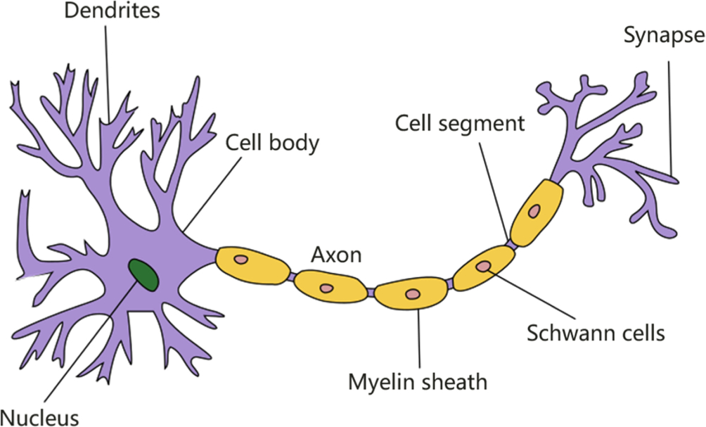
The most basic unit in a biological neural network is a neuron, and its structure is shown in Fig. 1.4. In the original mechanism of biological neural networks, each neuron has multiple dendrites, one axon, and one cell body. The dendrites are short and multibranched, with one axon that is long. Functionally, dendrites are used to introduce nerve impulses transmitted by other neurons, while axons are used to transmit nerve impulses to other neurons. When a nerve impulse introduced by a dendritic or cellular body excites a neuron, the neuron transmits excitability to other neurons through the axon.
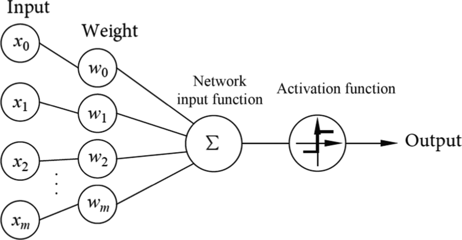
In the 1940s, American psychologist Warren McCulloch and mathematician Walter Pitts proposed the M-P neuron model based on the structure and working principle of biological neurons [4]. The mathematical model is shown in Fig. 1.5. The M-P neuron model, which was named after its coinventors, contains multiple inputs that correspond to dendrites, and the multiple dendrites are used to sense nerve impulses. More formally, this design is equivalent to the input signal Xi transmitted by n other neurons via an axon per neuron. In biological neurons, nerve impulses enter the cell body through complex biological effects, which is equivalent to the weighted summation and output of these signals in the M-P neuron model through the role of weights Wi. These weights are termed connection weights. A dendrite receives a nerve impulse transmitted by a synapse, which is equivalent to multiplying the input signal with the weight to get an output xiwi. Biological cells will feel the excitation of a nerve impulse transmitted by multiple synapses. The excitatory response in biological cells is then transmitted to other neurons through axons. This behavior is imitated in the M-P model, as the input signal of M-P neurons is processed with a neuron threshold b. Subsequently, the neuron output is generated for the next M-P neuron by applying an activation function. Therefore, the working principle of M-P neurons abstracts the biological neurons mathematically, and can be reconstructed and computed manually.
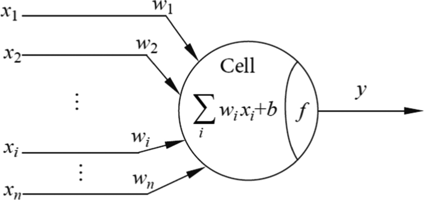
The schematic diagram of the M-P neuron model is shown in Fig. 1.5, where x1, x2, … xn denotes input signals from n neurons, respectively. Further, w1, w2, … wn denote the weights of the connections between n neurons and the current neuron, b denotes the bias threshold, y denotes the output of the current neuron, and f denotes the activation function. Putting everything together, the mathematical expression for the whole neuron is
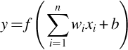
The function of formula (1.1) is to simulate the working mechanism of biological neurons: The neuron receives multiple input signals, weighted summation is performed, and a threshold is added. When the threshold b in formula (1.1) is negative, adding b is equivalent to subtracting the positive threshold. The output control is carried out through the activation function, which shows the process of neuron computation and processing. If multiple inputs are represented as a vector x = [x1, x2, …, xn]T, and multiple connection weights are represented as a vector w = [w1, w2, …, wn], then the output of the neuron becomes y = f(x · w + b). In detail, first perform vector multiplication on input signal vector and connection weight vector, and add bias value, then pass it through the activation function to obtain the final output.
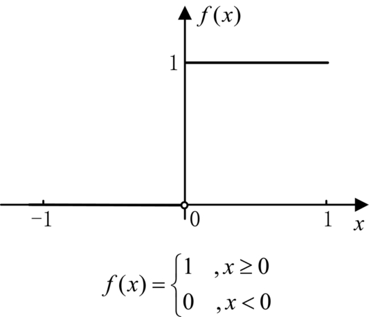
Activation functions are used to simulate the excitation of cells and signal transduction in biological neurons. Analysis of biological nerve signal transmission mechanisms found that there are only two states of nerve cells: the first is to achieve the excited state of nerve cells and to open the nerve impulse transmission; the second is a failure to make the nerve cells excited, which does not produce nerve impulses. In M-P neurons, the control function that activates this optimal output is a step function, as shown in Fig. 1.6, which maps the difference between the weighted summation value and the threshold to 1 or 0. If the difference is greater than or equal to zero, the output is 1, corresponding to the excited state of the biological cell; if the difference is less than zero, the output is 0. This design corresponds to the inhibition state of biological cells.
The M-P neuron model is the first mathematical model to characterize biological neurons. This model simulates the working mechanism of biological neurons, lifts the mysterious veil of biological neural systems, lays a foundation for the development of subsequent neural networks, and has a far-reaching importance in the establishment of the atomic structure of neural networks.
1.3.2: Perceptron
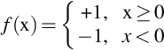
The structure of the perceptron is shown in Fig. 1.7. It is an ANN model based on the M-P neuron model [5]. The perceptron is a description of a network of neurons consisting of two levels: The first layer is the input layer, which consists of m + 1 inputs, x0, x1,…, xm. These neurons only receive signals and do not do any processing. The second layer is the output layer, which consists of an input function and an activation function of m + 1 weights w0, w1,…, wm. The network input function can be expressed as a weighted summation. The activation function is different from the M-P neuron. The perceptron uses the antisymmetric symbol function, as shown in Eq. (1.2). When the input is greater than or equal to 0, the output is + 1. When the input is less than 0, the output takes a value of − 1. Generally, the perceptron is a network with multiple inputs and a single output.
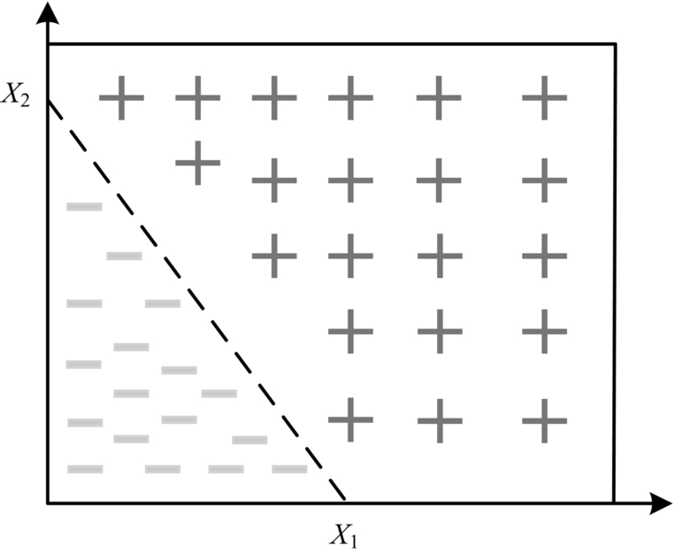
The basic mathematical principles of the perceptron and the M-P neuron model are the same, and they inherit the neuron model y = f (x · w + b). At the same time, since the perceptron divides the positive and negative examples of the training set into two parts and can be used to classify input data, the perceptron is a binary classifier. A perceptron is akin to how a person learns to recognize an object. For example, when a teacher instructs a student to recognize an apple, the teacher first shows a positive example by taking out an apple and telling the student, “This is an apple.” Subsequently, the teacher shows a counterexample by taking out a banana and telling the student, “This is not an apple.” Following these initial examples, the teacher may continue to show another example by taking out a slightly different apple and telling the students, “This is also an apple.” After a long period of training, the students finally learn to judge what an apple is, and thus know how to distinguish between apples and nonapples. This skill of “recognizing apples” is a trained model of perceptron. The emergence of the perceptron directly finds a preliminary direction for the application of neurons. The perceptron based on the M-P neuron model is a practical, simple ANN, which can solve straightforward binary linear classification problems. As shown in Fig. 1.8, two kinds of objects are classified by a linear method. The perceptron can find the dashed lines between (x1,0) and (0,x2) points in Fig. 1.8, and correctly distinguish between + and − objects. At the same time, the task of perceptron can be transferred, and it can be retrained by the Hebb learning rule or least-squares method. By adjusting the weights of the perceptron network without changing the network structure, the same perceptron can have the function of solving different binary classification problems.
In addition, it is particularly important that the perceptron also has hardware achievability. The first perceptron model, Mark1, implemented on the hardware, brought the neural network from theory to application. Because of the potential value of the perceptron, it immediately attracted the attention of many researchers.
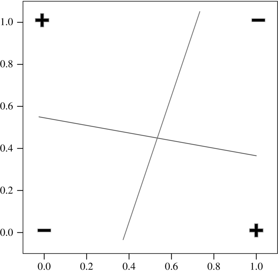
Unfortunately, perceptrons are limited to linear binary classification. For example, a perceptron cannot solve simple XOR problems. The XOR operation is shown in Fig. 1.9, with + for 1 and − for 0. Four logical rules are required for the XOR function: (1) 0 XOR 0 = −, corresponds to the lower left corner in the coordinate system; (2) 0 XOR 1 = +, corresponds to the upper left corner in the coordinate system; (3) 1 XOR 0 = +, corresponds to the lower right corner in the coordinate system; (4) 1 XOR 1 = −, corresponds to the upper right corner in the coordinate system. These four rules produce two results of + and −. If you want to classify these outputs by a linear classifier, the perceptron will not be able to find a line in the coordinate system that can separate the + and − attributes into the two distinct areas. Therefore, the application of the perceptron is extremely limited, making it necessary to find new ways to solve more complex classification problems.
1.3.3: Multilayer perceptron
1.3.3.1: Working principle
The perceptron can only deal with linear classification problems, and the output results are limited to 0 and 1. In order to solve more complex problems based on the traditional perceptron structure, such as multiclass classification problems, the structure of multiple hidden layers is used instead of a single layer. This deep structure is called multilayer perceptron (MLP), also known as a fully connected neural network (FCNN) [2]. MLPs are the earliest examples of DL feedforward neural networks. An MLP can classify an input into multiple categories. In an MLP, data can only flow in one direction, from the input layer, through the hidden layer, to the output layer, and does not form any cycles or loops within the network.
The input nodes in the MLP constitute the input layer, which receives data from the outside, but does not process the data. These nodes merely pass the data directly to the hidden nodes. Hidden layers are composed of several hidden nodes. Hidden nodes do not receive external data; they only receive data from input nodes, compute, and pass their results to output nodes. An MLP can have no hidden layers or it can have multiple hidden layers, but it must contain an input layer and an output layer. Output nodes form the output layer, which receives data from the upper layer (either the input layer or the hidden layer), computes, and passes the results to the external system. Hidden nodes and output nodes can be equivalent to neurons because they have similar computational processing functions. The perceptron can be regarded as the simplest MLP. It has no hidden layer, but has multiple inputs and one output. It can only classify input data into simple linear-classifiable categories.
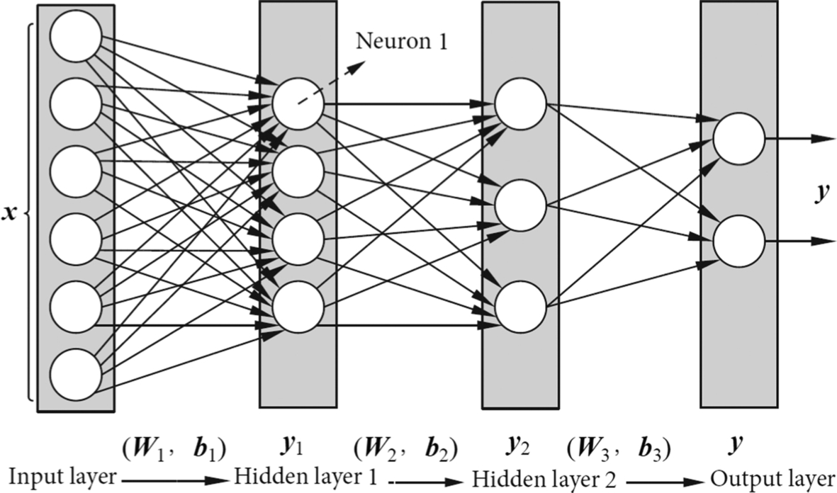
An MLP with two hidden layers is shown in Fig. 1.10. The structure is “Input Layer → Hidden Layer 1 → Hidden Layer 2 → Output Layer.” Fully connected data transmission is used between each layer, that is, each layer of neurons is connected to each neuron in the upper layer. In Fig. 1.10, neurons in Hidden Layer 1 process the input data to generate the output of neurons. For example, neuron 1 receives input to produce an output. There are four neurons in Hidden Layer 1, so there are four output results. These four outputs are processed by the neurons in Hidden Layer 2, with a total of three outputs. Following the same procedure, an MLP produces the final output. Therefore, the final output of the whole MLP can be regarded as the result of nested computation of multilayer neurons.
From a computational point of view, due to the one-way flow of feedforward network data, the MLP is essentially a nested call of the perceptron model, that is, the input data vector undergoes multiple perceptrons (e.g., formula (1.1)) in repeated processing in order to get the output. At present, there are many neurons in each layer of an MLP, whose input is vector x and output is vector y. The weight of each neuron is a vector w, and the weight vector w of multiple neurons constitutes a weight matrix W. Similarly, multiple biases of a layer of neurons constitute a biased vector b. Therefore, the fully connected computation model of multiple neurons in one layer can be expressed by formula (1.3). After multiplying the input vector x and the weight matrix, the bias vector can be added. The output vector y can be obtained by processing the activation function f, which completes the computation of multiple neurons in one layer of the network.
In Fig. 1.10, the vector x and the vector y are used to represent the input data and output data of the MLP, respectively. The terms W1, W2, W3 are used to represent the weight matrices of the connection weights between the neurons of different layers, while b1, b2, b3 represent the offset vectors of the different layers, and the vectors y1, y2 represent the calculated output of hidden layer 1 and hidden layer 2, respectively. When the input vector enters hidden layer 1 from the input layer, the weight matrix W1, and the offset vector b1, will have been applied. After the computation of the fully connected model, the output vector y1 is used as the input vector of the hidden layer 2. This process is continued through the entire fully connected network. Finally, the result y of the MLP is obtained through the output layer. This process is typical for a fully connected network.
1.3.3.2: Computational complexity
MLPs overcome the disadvantage that perceptrons cannot discriminate linearly nonseparable data. Accordingly, MLPs can solve nonlinear classification problems (e.g., the XOR problem). At the same time, with the increase in layers, any function can be approximated by MLP in finite intervals, which makes it widely used in speech and image recognition. However, when people begin to think that this kind of neural network can solve almost all problems, the limitations of MLP begin to appear. Since the MLP is fully connected and has a large number of parameters, the training time is very long and the computation is heavy. At the same time, the model can easily fall into the locally optimal solutions, which leads to difficulties with the optimization process of the MLP.
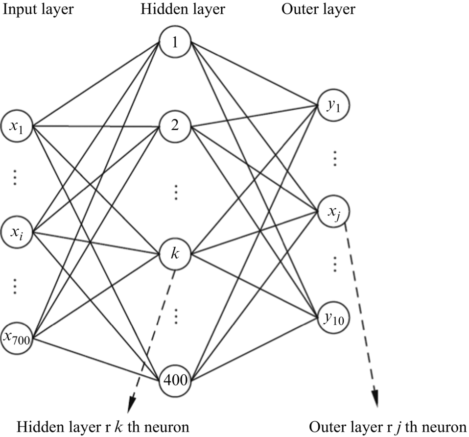
To illustrate the computational complexity of MLP, a simple MLP can be selected for demonstration purposes. As shown in Fig. 1.11, the structure for the network is “input layer → hidden layer → output layer” for a total of three layers. In this case, the input layer has 700 inputs and the hidden layer consists of 400 neurons, which are fully connected to the input layer. Each of these 400 neurons has 700 connections, and each connection has a weight. Therefore, the connection weight matrix of the hidden layer and the input layer is 700 × 400, while the neurons of each hidden layer also have an offset, so the offset vector of the hidden layer is 400. Next, in this example, assume the output layer has 10 outputs. Since the output layer and the hidden layer are also fully connected, the weight matrix between the output layer and the hidden layer is 400 × 10, and the offset vector of the output layer is 10. Therefore, the total number of weights of the entire MLP is 700 × 400 + 400 × 10 = 284,000, and the total number of offsets is 400 + 10 = 410. A weight of a neuron needs to be multiplied with the input data, so the entire MLP must perform 284,000 multiplication operations. At the same time, during the weighted summation, addition operations are required (which are less complex than multiplication). The total number of additions is equal to the number of multiplications, that is, (700 − 1) × 400 + 400 + (400 − 1) × 10 + 10 = 284,000.
In this simple example, even though the MLP with only one hidden layer is used to solve the 10-class classification problem of 700 inputs, the parameters multiplication and addition have reached nearly 300,000, respectively. This amount of computation and parameters is very large. When considering that a standard image may have a size of roughly 1000 × 1000 pixels, it is clear that 700 inputs is very small. With a more typical image, its pixel size could be on the order of 1 million, and 1000 nodes could be used as output for 1000 classes. So even if the whole MLP contains only one hidden layer of 100 nodes in one layer, the number of parameters are easily over 100 million. Even by the power of today’s mainstream computers, the amount of computation and parameters are considerable.
In addition, for image recognition tasks, each pixel is closely related to its surrounding pixels, while the correlation with distant pixels is relatively small. However, MLPs can only take input in the form of vectors, so the image of a two-dimensional matrix must be converted into vectors prior to being fed into the network for computation and processing. In other words, the input of this vector causes all the pixels in the image to be treated equally, without incorporating the position-related information between the pixels in the image. Consequently, many connections have little effect on feature extraction. At the same time, too many parameters and computations negatively affect the computational performance of predictions and applications.
With the addition of more layers of the MLP, the stronger the representation ability it has. However, it is very difficult to train an MLP with a large number of layers by the commonly used gradient descent method. The number of layers directly affects the parameters and computation. Generally speaking, gradients are difficult to transmit over three layers, so it is impossible to get a deep MLP. Due to the problem of high computational load with MLP s, researchers continued to search for more efficient neural network algorithms.
1.3.4: Convolutional neural network
Since the MLP is built in the form of a fully connected feedforward network, there are too many parameters, which leads to limitations such as long training time and difficulty in network tuning. At the same time, due to its fully connected form, the network deals with global features of the image, which makes it difficult to capture the rich local features. These limitations forced researchers to seek new network structures. In this scenario, multilayer neural networks emerged. Multilayer neural networks overcome the limitations of MLPs, and the CNN is representative of various multilayer neural networks [2].
The CNN is based on a neuron model and connects thousands of neurons through a hierarchical structure by following certain rules. From the perspective of computer science, the essence of CNNs is always a recursive call of the M-P neuron model.
The earliest CNN was LeNet5, which was published by LeCun in 1998, in the paper LeNet5-Gradient-Based Learning Applied to Document Recognition. However, CNNs were not popularized until 2012, when AlexNet (8-layer CNN) won the championship with a top-5 error rate of 15.3% in the ILSVRC competition classification challenge. The CNN prompted an upsurge of neural network studies, driven by an accuracy in the ILSVRC competition that was far higher than second place. AlexNet became a foundation of deep neural networks and reignited interest in DL.
Despite their longer history, CNNs were not particularly popular until 2012. One of the factors that sparked interest in CNNs in 2012 was the progress of heterogeneous computing that enabled people to use the power of a large number of GPUs for network training. Further, there was simultaneously an explosive growth in data availability for network training. On the other hand, the increasing depth of neural networks was well handled, as certain solutions and techniques were proposed to enable stable training of deep convolution neural networks. At present, common deep neural networks, such as AlexNet, VGG, GoogleNet, and LeNet, are all CNNs.
The CNN has made many improvements upon MLPs. It introduces new features such as local connections, weight sharing, and pooling. These techniques largely solve the inherent flaws of the perceptron. At the same time, the CNN has strong feature extraction and recognition ability, so it is widely used in the image recognition field. Common applications include object detection, image classification, and pathological image diagnosis.
1.3.4.1: Introduction to network architecture
CNNs require three processes: build the network architecture, train the network, and perform inference. For a specific application, a hierarchical architecture of CNNs, including an input layer, convolution layers, pooling layers, fully connected layers, and output layer, are required. By flexibly arranging or reusing these layers, a wide variety of CNNs can be generated. After defining the CNN structure, a large amount of data is needed to train the network to obtain optimal weights of the network. After training is complete, the model of the optimal network structure is obtained and can be used to infer new data and perform tests or predictions. In fact, the ultimate goal of CNNs is to provide an end-to-end learning model for specific applications. This learning model completes the task for a specific application, such as feature extraction and recognition/classification.
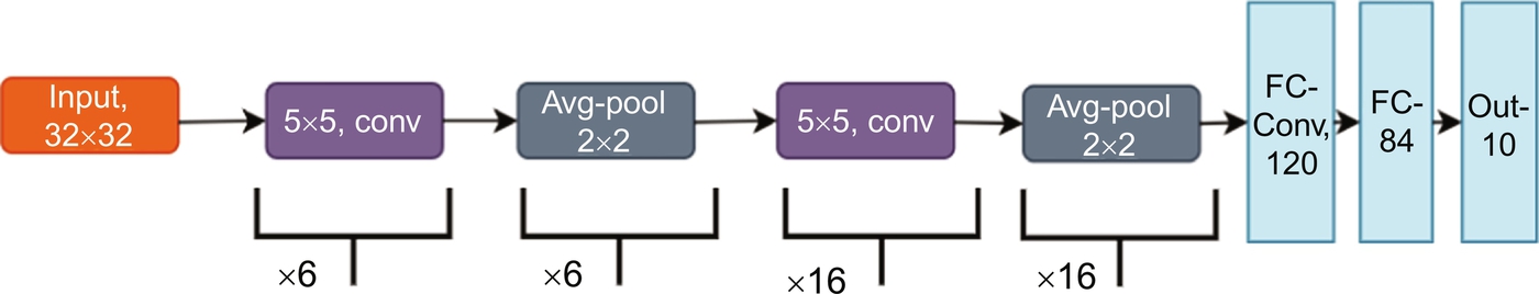
As shown in Fig. 1.12, the LeNet5 network structure is the most classic CNN [6]. The LeNet5 network consists of one input layer, two convolution layers, two pooling layers, two fully connected layers, and one output layer. The network structure is “Input Layer → Convolution Layer 1 → Pool Layer 1 → Convolution Layer 2 → Pooling layer 2 → Fully connected layer 1 → Fully connected layer 2 → Output layer.” The data is fed to the input layer, passes through the convolution layers, the pooling layers, and the fully connected layers, and finally to the output layer. The data flows in one direction. Therefore, LeNet5 is also a typical feedforward neural network, and later CNN architectures are developed on this basis. Each functional layer (such as convolutional layer, pooling layer, etc.) has an Input Feature Map and an Output Feature Map. All input feature maps of the same functional layer have the same size, and all output feature maps of the same functional layer have the same size. However, the size and number of the input and output feature maps for the same functional layer may vary, depending on the properties of the functional layer itself.
Like traditional image processing, the input image data needs to be preprocessed before it is sent to the input layer, so that the data obtained in the input layer can meet the format requirements of the CNN. In general, the input image data is also referred to as an input feature map, and may be a three-dimensional 8-bit integer data in RGB format. For example, with input image data of size 224 × 224 × 3, the data format is [224, 224, 3]. The first 224 is the image width; the second 224 is the image height, and the number of pixels in the whole image is the height multiplied by the width, i.e., 224 × 224. The final dimension, 3, indicates the number of channels of the input feature map, such as R, G, and B. There are totally three color channels. Therefore, the dimensions of an input feature map consist of width, height, and number of channels.
The neural network generally averages the input data, so that the mean value of the sample data is adjusted to zero. In addition, in order to facilitate the learning of a CNN, the input data is also normalized to a specific range, such as [− 1.0, 1.0]. Thus, the actual input to the network may be represented as a single-precision, floating-point number. Sometimes, in order to adapt to the requirements of the neural network, the size of the input data is also adjusted to a specified size. For example, the data could be reduced to a constant size by principal component analysis (PCA) [7]. In short, the input layer is used to prepare the data so that it can be easily processed by the CNN. Once the input data is processed, it is then processed by the convolutional layers, the pooling layers, etc., and finally the result is computed by the fully connected layers and the output layer.
1.3.4.2: Convolutional layer
The input layer conveys data to the convolutional layer and is then processed by the convolutional layer. As the core layer in the neural network, the convolutional layer can enhance the feature information and filter out useless information. The convolution layer extracts key features from the input feature map through multiple convolution operations, and generates an output feature map. The convolutional layer usually convolves the image by two-dimensional convolution, and performs convolutions upon a set of neighborhood pixels centered on each pixel. Each neuron performs the weighted summation of neighborhoods of each pixel and outputs the result. The offset is added to adjust the range of the final result. This final result is called the feature value. The output feature values of a number of neurons in the convolutional layer constitute a feature map.
The weighted summation in the convolution process uses a convolution kernel, which is also called a filter. A single convolution kernel is usually a three-dimensional matrix and needs to be described by three parameters, width, height, and depth. The depth is the same as the number of channels of the input feature data. The convolution kernel depth shown in Fig. 1.13 is three. Different convolution kernels extract different features. As some convolution kernels are sensitive to color information, and some convolution kernels are sensitive to shape information, a CNN can contain multiple convolution kernels to model multiple features.
The value of the convolution kernel is stored in the form of a two-dimensional weight matrix, which is represented by width and height. The number of weight matrices in a convolution kernel is consistent with the depth of the convolution kernel, which is equal to the number of channels in the input feature map. The distance at which the convolution kernel slides at a time on the feature map is called the step size. The convolution kernel weights generally use a matrix of size 1 × 1, 3 × 3, or 7 × 7, and the weight of each convolution kernel is shared by all convolution windows on the input feature map. Sizes of convolution kernels are the same in one layer, but they can be distinct in different layers. In Fig. 1.14, the size of all convolution kernels in the first layer is unified to 3 × 3.
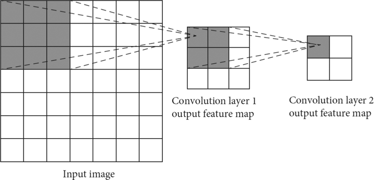
The portion of the original input feature map (or the first input feature map) corresponding to a convolution window is called the receptive field. The receptive field is a rectangular area on the original input feature map. Because there may be multiple convolutional layers in the network, the convolution window size and the receptive field size of the same input feature map may be different. But the convolution window of the first layer is generally of the same size as the receptive field. The receptive field is represented by two parameters, height and width. The height and width of the convolution window are consistent with the height and width of the convolution kernel of the same layer. As shown in Fig. 1.14, the 3 × 3 convolution kernel on the first convolutional layer has a receptive field size of 3 × 3 on the input image. Similarly, the 2 × 2 size convolution kernel in the second convolution layer corresponds to a convolution window size of 2 × 2 on the output feature map of the first layer, but this actually corresponds to a receptive field size of 5 × 5 on the original image.
Neurons cannot perceive all the information of the input feature map; they can only act on the receptive field of the original input feature map through the convolution kernel at each layer. Thus, the larger the receptive field, the larger the area of the convolution kernel acting on the original image. When the convolution kernel slides horizontally and vertically with a specific step size on the input feature map, at each step the weight matrix will be multiplied by the corresponding elements in the corresponding input feature map, and finally the output feature values can be obtained by deducting the offset. When the convolution kernel traverses all the positions of the input feature map, it generates a two-dimensional output feature map. Usually, the output feature maps of all channels corresponding to the same convolution kernel are added to form the final output feature map for the convolution kernel. Multiple convolution kernels generate multiple output feature maps, which are provided as input for the next layer.
After the convolution operation, each feature value in the output feature map needs to be activated by the activation function. Because the step function is discontinuous and not smooth, it is difficult to train. In practice, we normally use sigmoid, tanh and ReLU (Rectified Linear Unit), to approximate the step function. The activation function filters the output feature values to ensure the effective transmission of information. At the same time, the activation function is usually nonlinear, while the convolution is linear. That is to say, in the convolutional layer, neurons only have a linear processing function, because the linear combination of linear functions remains linear, no matter how deep a neural network is used. Without a nonlinear activation function, a purely linear deep neural network is equivalent to a shallow network. The activation function introduces nonlinear factors into a neural network, which enhances the ability of DL to fit nonlinear features.
Properties of the convolution layer
As seen from MLPs, the number of weights has a great influence on the computation complexity and storage size of the model during training and inference. CNNs adopt local connection and weight sharing to reduce the storage space of the network model and improve the computing performance.
- (1) Local connection
Full connections are adopted in MLPs, meaning that almost the whole image is processed by each neuron. As shown in Fig. 1.15, neuron 1 acts on all the pixels of the input image and has a weight in connection with each pixel. Thus, a single neuron generates many weights, as well as many neurons, resulting in a huge number of parameters. The convolution neural network adopts the sparse connection, which makes each neuron in the convolution layer only process the data in the receptive field of the input feature map. This is another advantage of the convolution neural network.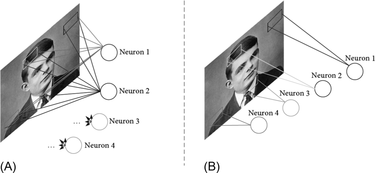
Fig. 1.15 Comparison of full connection and local connection. (A) Fully connected. (B) Locally connected. Turing photo source: https://upload.wikimedia.org/wikipedia/commons/thumb/a/a1/Alan_Turing_Aged_16.jpg/220px-Alan_Turing_Aged_16.jpg.
In Fig. 1.15, Neuron 1, Neuron 2, Neuron 3, and Neuron 4 only affect the pixels of a small area, which makes the weight parameters of the whole area decrease sharply. The theoretical basis of using a local connection in CNNs is that in a feature map, each pixel is closely related to its adjacent pixels, while the correlation between distant pixels is weak. Therefore, the influence of the distant pixels on the extraction of output features is shielded, and it also reduces the number of network model parameters. - (2) Weight sharing
Different feature values on the output feature map are generated by different neurons in the convolutional layer. Different neurons in the same convolutional layer use the same convolution kernel, so there is weight sharing between these neurons. Weight sharing greatly reduces the number of parameters in the CNN. As shown in Fig. 1.16, if weight sharing is not used, Neurons 1, Neurons 2, Neurons 3, and Neurons 4 on the same convolutional layer have different weights, corresponding to Weight 1, Weight 2, Weight 3, and Weight 4. In the weight sharing mode, the four neurons share the same weight of 1, directly reducing the total weight of this neuron to 1/4 of the weight-independent model, which greatly reduces the number of parameters in the neural network.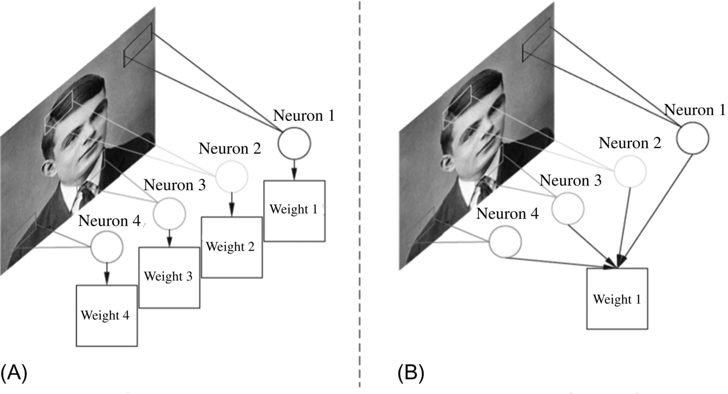
Fig. 1.16 Weight sharing. (A) Weight-independent. (B) Weight-sharing. Turing photo source: https://upload.wikimedia.org/wikipedia/commons/thumb/a/a1/Alan_Turing_Aged_16.jpg/220px-Alan_Turing_Aged_16.jpg.
The reason why weight sharing has little influence on the output feature map is that each image has inherent features, and these inherent features will be near identical in every part of the image. Therefore, using the same feature extraction method for different parts of the image, or even convolution with the same weights, can be effective in obtaining the features. The loss of information provided by the features is small, which ensures the integrity of the image features, while significantly reducing the number of weights. Therefore, no matter how many neurons there are in the convolution layer, for each image, only a set of weights needs to be trained. In this way, the time required for training parameters is greatly reduced. However, sometimes weight sharing also fails, for example, if the input image has a central structure and the goal is to extract different features from different positions of the image by convolution. In this case, the corresponding neurons of different image positions may need different weights.
Implementation of the convolutional layer
- (1) Direct convolution
There are several ways to implement a convolutional layer. The most straightforward way is direct convolution. Direct convolution is computed based on the inherent property of the convolutional layer, and the input feature map needs to be padded before computation. One of the benefits of zero padding is that the input feature map can be consistent with the size of the output feature map after the convolutional layer is processed. At the same time, zero padding can protect the edge information of the input feature map, so that it is effectively protected during convolution. If the input feature map is not padded, the input data will decrease in size during convolution, causing loss of information at the edge. Therefore, zero padding is a common preprocessing method before convolutional layers.
The weight matrix of the convolution kernel slides over the input feature map after zero padding. At each position in the input feature map, a submatrix, matching the size of the convolutional kernel, is multiplied by the corresponding elements (also called a “dot product”). Here, this submatrix is called the input feature submatrix, and the number of input feature submatrices in one input feature map is the same as the number of elements in the output feature map.
As mentioned later in this book, most CNN accelerators are designed using direct convolution computations. For example, the Tensor Processing Unit (TPU) proposed by Google uses the computation method of the systolic array. This computation method utilizes input and output feature map parallelism and weight parallelism, and maximizes the reuse of the weight and input data in the architecture design, which can reduce the bandwidth requirement of the computing unit and achieve high computational parallelism.
Specifically, as shown in Fig. 1.17, for an input feature map matrix X having only one channel, its size is 5 × 5. There are two convolution kernels, where convolution kernel 1 has weight W1, and all elements in the b1 offset are 0; convolution kernel 2 has a weight of W2, and all elements in the b2 offset are 1. The weights of the kernels are shown in the 3 × 3 matrices, the step size of the convolution kernels is 2, and the padding size at the boundary is 1.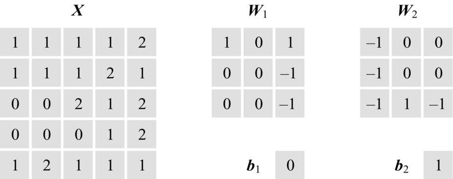
Fig. 1.17 Input data of the convolution.
As shown in Fig. 1.18, when convolution is performed, the input feature matrix X is first padded with zeros. Since the size of the zero padding is 1, the feature matrix is extended outward by one pixel to obtain the matrix Xp. In the process of convolution, the weight W1 acts on the initial position x1 of the Xp matrix, and the dot product between the input feature submatrix X1 in Xp and W1 is computed. The result of this dot product forms the first element of the output feature matrix Y1 after the biasb1 is added. The result is − 2, as computed by: 0 × 1 + 0 × 0 + 0 × 1 + 0 × 0 + 1 × 0 + 1 × (− 1) + 0 × 0 + 1 × 0 + 1 × (− 1) + 0 = − 2. After the first element of Y1 is computed, the weight W1 matrix slides the step size of the two elements to the right. At this time, the weight W1 matrix overlaps with the input feature submatrix X2 in the matrix Xp, and the dot product of the corresponding elements is performed. Then, after adding the offset, the value of the second element of the output feature matrix Y1 is computed to be − 3. Following this rule, the computation of all elements in the first row of the output feature matrix Y1 is completed. When performing the element computation of the second row of the output feature matrix Y1, it should be noted that the weight W1 needs to slide the step size of two elements vertically downward from the position of the input feature submatrix X1. The first element of the second row is computed as 1, as shown in Fig. 1.18. The step size plays a role in both the lateral and longitudinal movements of the convolution kernel on the input feature map. Thus, after nine movements and dot products, all elements of the output feature map Y1 are obtained. For convolution kernel 2, the output feature map Y2 can be obtained using the same method.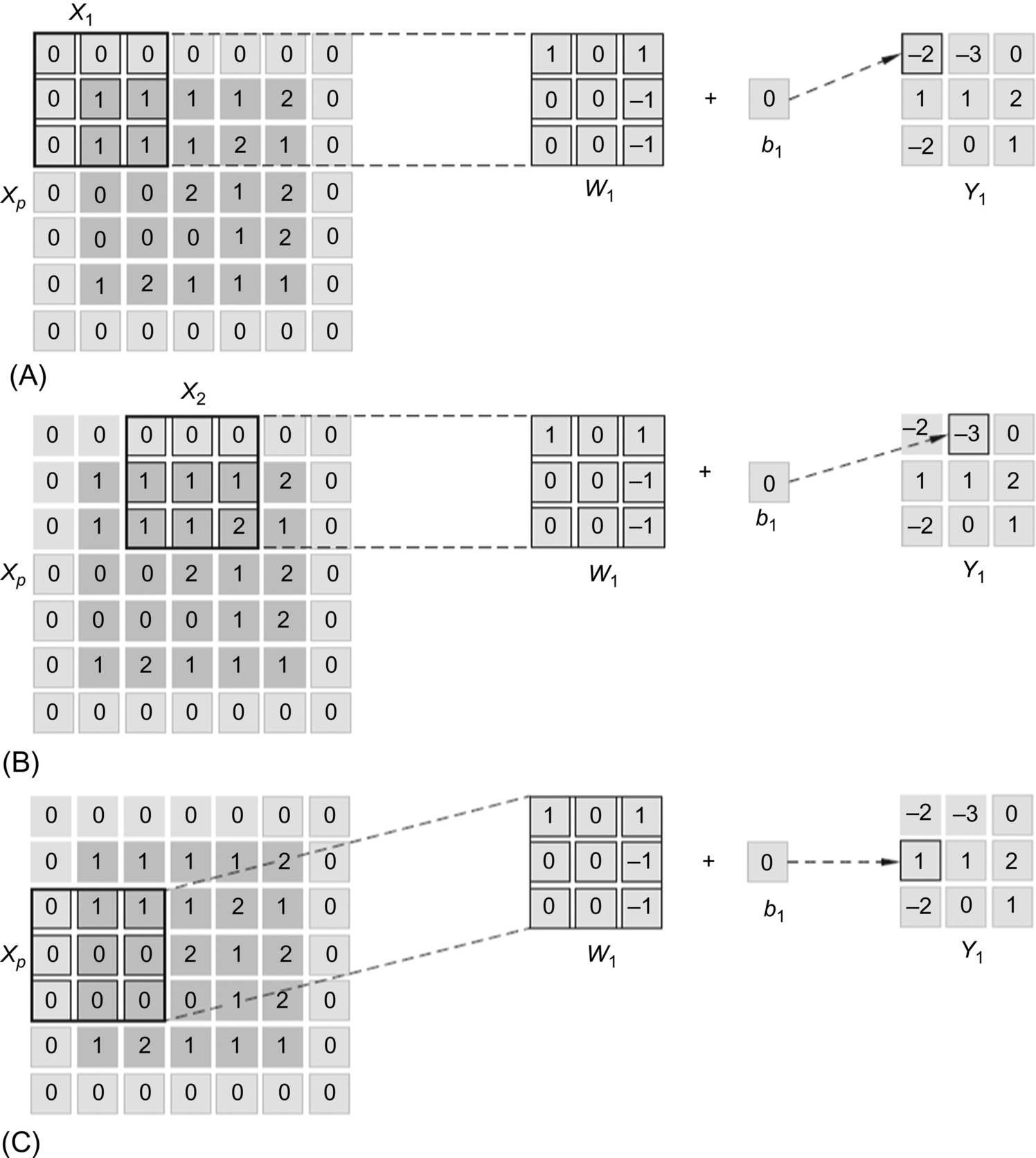
Fig. 1.18 Direct computation of convolution. (A) Output first element. (B) Row sliding computing. (C) Column sliding computing.
So far, the convolution of the input feature map and the weight matrix is completed by the direct convolution method. In real applications, each convolution kernel has multiple channels, and the weight matrix of all channels needs to be used to convolve the corresponding channel of the input feature map. The results of all channels are accumulated as the final output feature map of the convolution kernel. - (2) Convolution by matrix multiplication
In addition to the direct convolution method described above, convolution can also be achieved by matrix multiplication, and this method is widely used in CPU, GPU, and other processors, including Huawei’s Ascend AI processor.
This method first expands the input feature map and the convolution kernel weight matrix in the convolution layer by Img2Col (Image-to-Column), and then converts the dot product of the input feature submatrix and the weight matrix in the convolution into the matrix operation of the multiplication and addition of the row and column vectors, so that a large number of convolution computations in the convolutional layer can be converted into the parallelized matrix operations. Therefore, the processor only needs to efficiently implement matrix multiplication, and the convolution operation can be performed efficiently. Both CPU and GPU provide specialized Basic Linear Algebra Subprograms (BLAS) to efficiently perform vector and matrix operations.
The Img2Col function expands each input feature submatrix into a row (or a column) and generates a new input feature matrix whose number of rows is the same as the number of input feature submatrices. At the same time, the weight matrix in the convolution kernel is expanded into one column (which may also be one row), and the multiple weight matrices may be arranged in multiple columns. As shown in Fig. 1.19, the input feature map Xp is expanded into a new matrix XI2C by Img2Col expansion. First, the input feature submatrix X1 is expanded into the first row of XI2C, and the input feature submatrix X2 is expanded into the second row. Since there are nine input feature submatrices, all of which are expanded into nine rows, the final XI2C matrix can be generated. Similarly, the weight matrices W1 and W2 of the two convolution kernels can be expanded into a matrix WI2C, and the offset matrix bI2C can be similarly processed. Next, the matrix multiplication operation is performed, and the first row of XI2C and the first column of WI2C are combined, yielding the first value of YI2C after adding the offset. The remaining elements of the output map matrix YI2C are obtained similarly.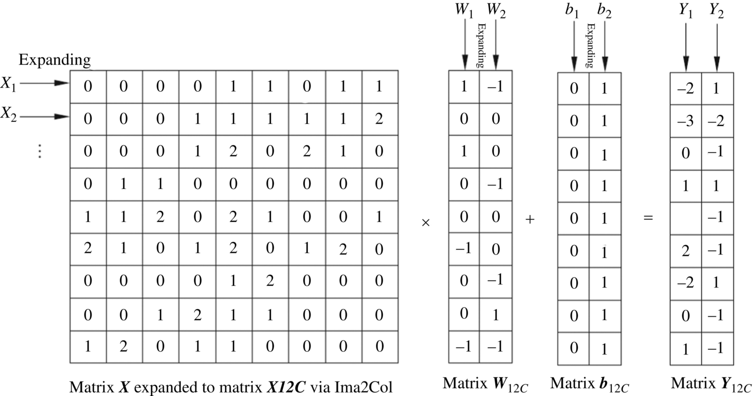
Fig. 1.19 Convolution by matrix multiplication.
The function of Img2Col is to facilitate the conversion of the convolution into matrix multiplication, so that the feature submatrices can be stored in continuous memory before matrix multiplication is performed. This reorganization reduces the number of memory accesses and thus reduces the overall time of the computation. In the case of direct convolution computation, since the input feature submatrices are stored in memory with overlapping but discontinuous addresses, it may be necessary to access the memory multiple times during the computation. These multiple memory accesses directly increase the data transfer time, which further affects the speed of convolution computation. Img2Col plays a vital role in facilitating the convolution computation, by converting the convolution computation into matrix multiplication.
When the offset value is constant in a convolution kernel, the computation of the offset can be further optimized. Specifically, the offset value and the weight matrix of the convolution kernel can be combined, and the coefficients are added to the input feature matrix. As a result of this optimization, the computation of matrix multiplication and bias accumulation is implemented at one time. As shown in Fig. 1.20, the coefficient matrix I is appended to the XI2C matrix, where the I matrix is a 9 × 1 dimensional and all elements are set to unity The bias matrix b is also appended to the WI2C matrix, where b = [0 1]. Then the computation is.
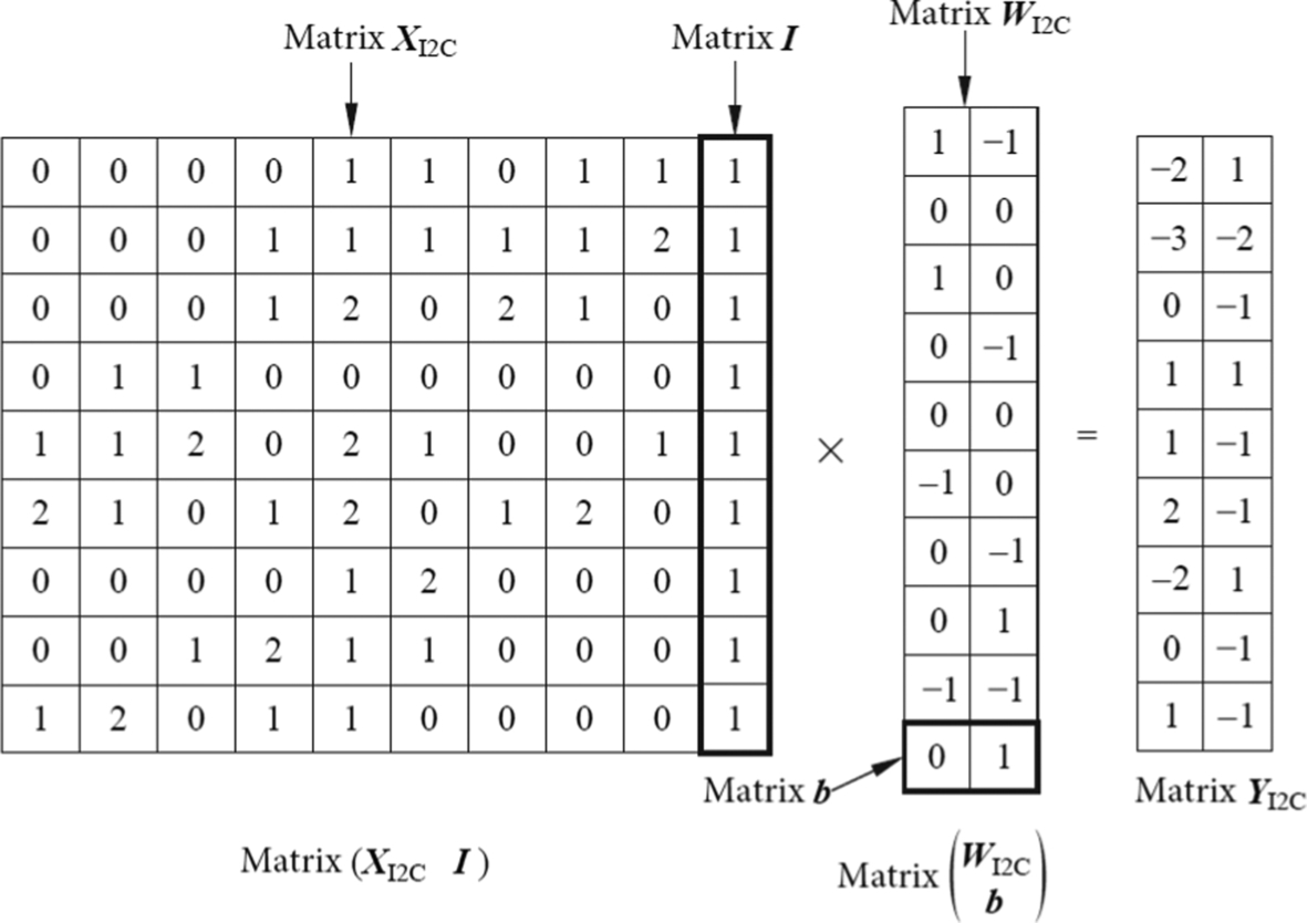
Fig. 1.20 Optimization of bias accumulation.
From Eq. (1.4), the multiplication of the matrix (XI2CI) with is equivalent to the result of multiplication of (XI2C) and (WI2C) followed by the addition of bI2C. By increasing the dimensions of the matrix, it is possible to perform computations using only matrix multiplications, saving computational resources on the hardware and simplifying the computation process.
It is worth mentioning that convolution in modern processors can also be achieved by other means such as fast Fourier transform (FFT) and the Winograd algorithm. These methods all reduce the computational complexity by transforming complex convolution operations into simpler operations. The convolution in the cuDNN library provided by NVIDIA partially uses the Winograd algorithm. Generally, in the CNN, the parameter and number of operations in the convolutional layer account for the vast majority of the entire network. Accordingly, acceleration of the convolutional layers can greatly improve the computation speed of the overall network and the execution efficiency of the entire system.
.jpg)
1.3.4.3: Pooling layer
As the CNN continues to get deeper, the number of neurons increases, and enormous amounts of parameters need to be trained. In addition, the overfitting problem still exists, even after employing the abovementioned methods of weight sharing and local connections. The CNN innovatively adopts a downsampling strategy, which regularly inserts a pooling layer between adjacent convolutional layers, reducing the number of feature values (the output of neurons) following the pooling layer. With this approach, the main features are retained while the size of feature maps is reduced, resulting in a reduction in the total number of computations, and a reduced chance of overfitting.
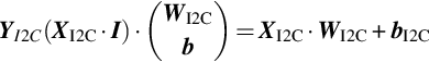
The pooling layer typically uses a filter to extract representative features (e.g., maximum, average, etc.) for different locations. The pooling filter commonly uses two parameters: size F and step size S. The method of extracting features from the pooling filter is called a pooling function. The pooling function uses the overall statistical features of the output in the neighborhood of a location to replace the value of the output at that location. The commonly used pooling functions include the maximum pooling function, average pooling function, L2 normalization, and weighted average pooling function based on the distance from the center pixel. For example, the maximum pooling function gives the maximum value in the adjacent rectangular region.
After the convolution layer is performed, the output data is handed over to the pooling layer for processing. In the input feature map of the pooling layer, the pooling filter usually slides horizontally and vertically with a window size FxF and step size of S. At each position, the maximum or average value in the window of the input feature map is obtained and forms the output feature value. Consider the example shown in Fig. 1.21, where the pooling filter is a 2 × 2 matrix and the step size is 2. In this example, a 4 × 4 input feature map is the input of the pooling layer. Output feature map 1 is computed by the maximum pooling function and has a size of 2 × 2, while output feature map 2 is generated by the average pooling function. The size of the output feature map is 2 × 2, which indicates that the pooling layer directly reduces the number of feature values of the output feature map to 1/4 of the input feature map size. This process reduces the amount of data while retaining the main feature information.
When using different pooling functions, the pooling filter does a small amount of translation on the input feature map. However, most of the feature information will not change after the pooling function, which means that it effectively retains the majority of the feature information of the input. This characteristic is called local translation invariance. Local translation invariance is a very useful property, especially when it is concerned about whether a feature appears or not. For example, when deciding whether a face is included in an image, it is not necessary to know the exact location of the pixels of the eyes, but to know that one eye is on the left side of the face and the other eye is on the right side of the face. However, in some other applications, the specific location of features is very important. For example, if you want to find a corner where two edges intersect, you need to preserve the position of the edges to determine whether the two edges intersect. In this case, the pooling layer will cause damage to the output features.
In short, the pooling layer summarizes all the feature information centered on each position of the input feature map, which makes it reasonable that the output data of the pooling layer is less than the input data. This method reduces the input data to the next layer and improves the computational efficiency of the CNN. This reduction in size is particularly important when the next layer is the fully connected layer. In this case, the large-scale reduction of input data will not only improve the statistical efficiency, but also directly lead to a significant reduction in the number of parameters, thus reducing storage requirements and accelerating computation performance.
1.3.4.4: Fully connected layer
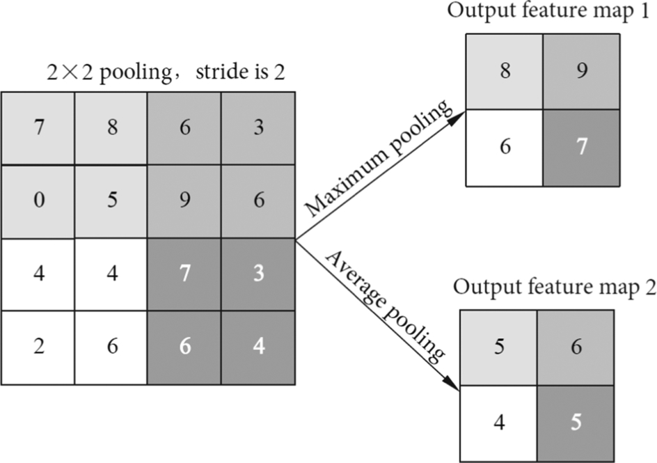
The data stream of a convolution neural network is processed by convolution layers and pooling layers for multiple iterations, which are then followed by fully connected layers. A fully connected layer is equivalent to an MLP, which performs classification upon input features. As shown in Fig. 1.22, the fully connected layer consists of 1 × 4096 neurons, each of which is fully connected to each neuron in the previous layer (often a pooling layer). After extracting the image features from the convolutional layers, the image features are classified by the fully connected layer, determining the class of the features. There are 1000 output classes in Fig. 1.22. After identifying the classes of the features, the probability of all classes is output through the output layer. For example, a fully connected layer will detect the features of a cat, such as a cat’s ear, cat’s tail, and so on. These data will be categorized as a cat, and finally the output layer will predict a large probability that the object is a cat.
1.3.4.5: Optimization and acceleration
The computation in convolution layers has five levels of parallelism: synaptic parallelism, neuron parallelism, input feature map parallelism, output feature map parallelism, and batch processing parallelism. These five parallelization methods make up the whole convolution process. The levels are sorted from low to high, and the amount of computing data for the various levels is graded from small to large. As the parallelization level rises, the requirement of computing resources becomes higher.
Consider the following example of a convolutional layer, in which the input image has N channels, the size of a single convolution kernel is K × K, the number of convolution kernels is M, and the size of the output feature map is SO × SO. Let us consider the manner in which the convolution layer is processed in order to understand how each parallelization level works.
Synaptic parallelism
When the weight matrix in a convolution kernel is computed in a single convolution window of an input feature map, the weights are multiplied by the input feature values in the convolution window, and a total of K × K multiplication operations are performed. There is no data dependency in the process, so the multiplication operation in the same convolution window can be performed in parallel. A multiplication operation is similar to a synaptic signal of a neuron acting on a dendrite. Therefore, this type of parallel methods is called a synaptic parallel. For convolution kernels of size K × K, the maximum synaptic parallelism is also K × K. In addition, after multiplication gives the products, it is necessary to perform the accumulation output immediately. Assuming that the addition unit can be shared by multiple convolution kernels, the pipeline mechanism can be used, that is, when the multiplication step is performed in a weight matrix, the previous weight matrix can do the summation using the addition unit. Multiplication and addition by multiple weight matrices can be performed in parallel.
Neuron parallelism
When an input feature map is processed by a convolution neural network, a convolution kernel slides over the input feature map, causing the generation of multiple convolution windows. Each of the convolution windows has no data dependency upon the other and thus can be computed in parallel. The dot product operation of each convolution window can be performed by a single neuron, so that multiple neurons can perform parallel operations on multiple convolution windows. This parallel mode is called neuron parallelism.
If the size of a convolutional layer output feature map is SO × SO, where each output feature value is computed by a convolution kernel in the corresponding convolution window, a total of SO × SO convolution windows are required. The computation can be performed simultaneously by SO × SO neurons in parallel, yielding parallelism in the convolutional layer of SO × SO. At the same time, in this parallel mode, since the convolution kernel weights used in multiple convolution windows can be shared (they are actually the same set of weights), and the input feature values of multiple convolution windows overlap, part of the data is reusable. By fully exploiting this data reusability in convolution computations, it is possible to reduce the size of the on-chip cache and the number of data read and write operations. These improvements lead to reduced processor power consumption and improved performance.
Input feature map parallelism
A typical CNN processes a multichannel input image, such as an RGB image. The number of channels in a convolution kernel is generally equal to the number of channels in the image. After each channel of the input feature map enters the convolutional layer, it is two-dimensionally convolved with the corresponding channel of the weight matrix in a convolution kernel. Each channel of the weight matrix is convolved only with the corresponding channel of the input feature map. This operation yields a channel of the matrix of output features. However, the output feature matrix for the multiple channels must be aggregated in order to obtain the final output feature map, which is the result of the convolution kernel.
Since the multichannel weight matrices in a single convolution kernel are independent in the convolution process and the multichannel input feature maps are also independent, channel-level parallel processing can be performed. The parallel processing is called input feature map parallelism.
As an example, for an RGB image, the number of channels in the input feature map is three, and parallel convolution can be performed for the three channels of the weight matrix in the convolution kernel. Therefore, the maximum parallelism for an input image with N channels is N. In the input feature map parallel mode, the data of multiple two-dimensional convolution operations does not overlap and has no dependencies. Therefore, the hardware can perform parallel computation of the input feature map as long as it can provide sufficient bandwidth and computational power.
Output feature map parallelism
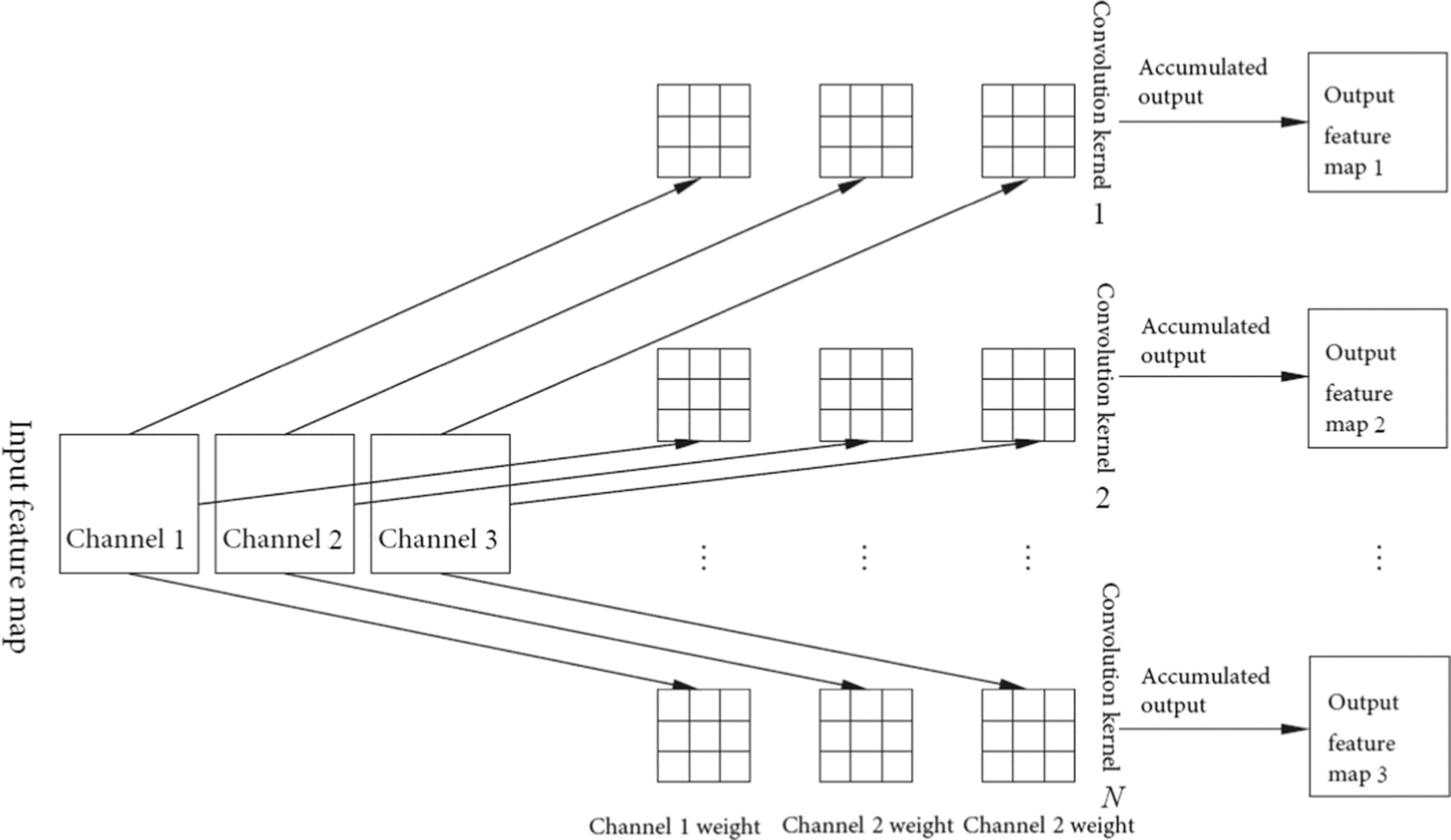
In a CNN, in order to extract multiple features of an image, such as shape contours and color textures, it is necessary to use a number of different convolution kernels to extract features. When the same image is set as input, multiple convolution kernels perform convolution computations on the same image and produce multiple output feature maps. The number of output feature maps and the number of convolution kernels are equal. Multiple convolution kernels are computationally independent and have no interdependencies. Therefore, the operations of multiple convolution kernels can be parallelized and independently derive the corresponding output feature maps. Such parallelism is called output feature map parallelism.
For computation of convolutional layers with M convolution kernels, the maximum degree of parallelism is M. In this parallel mode, the weight values of multiple convolution kernels do not coincide, but the input feature map data can be shared by all convolution kernels. Therefore, taking full advantage of the reusability of the input data can help achieve the best performance.
Batch parallelism
In the practical application of CNNs, in order to make full use of the bandwidth and computing power of the hardware, more than one image are processed at a time, which form a batch. If the number of images contained in a batch is P, the parallelism of the batch is P. The same CNN model uses the same convolution layer for different images processed in batches, so the network weights used by different images can be reused. The advantage of such large-scale image processing is that the on-chip cache resources can be fully utilized, and the weight data that has been transferred to the processor can be fully utilized, thus avoiding frequent memory accesses. These optimizations reduce the power consumption and delay of data transfer.
On the other hand, computing hardware can process multiple tasks in parallel, improving the utilization of hardware resources and the overall computing throughput. Task-level parallelism is also a way that CNNs can be accelerated, but compared with task-level parallelism, batch processing has higher requirements for hardware resources.
According to the actual situation, flexibly using the parallel methods of convolutional layers can efficiently accelerate the computation of a CNN. Considering the extreme case, since each of the parallel methods is performed at different levels, theoretically all parallel methods can be used simultaneously. Therefore, the theoretical maximum parallelism in a convolutional layer is the product of the parallelism exhibited by all parallel methods. As shown in Eq. (1.5), K × K is the synaptic parallelism, SO × SO is for the neuron parallelism, N is the input feature map parallelism, M is the output feature map parallelism, and the total number of input images in one batch is P. Achieving maximum parallelism is equivalent to all multiplications in the convolutional layers of all tasks being computed simultaneously.
For example, in Fig. 1.23, the number of channels of the input feature map is N = 3, the width and height of the convolution kernel weight matrix are K = 3, the number of convolution kernels is M = 4, and the output feature map dimension is SO = 6. In the processing of the convolutional layer, synaptic parallelism is first performed; that is, a 3 × 3 parallel multiplication with a degree of parallelism of 9. Simultaneously with neuron parallelism, a 6 × 6 output feature map can be convolved by 6 × 6 neurons with a degree of parallelism of 36. When the input feature maps are parallelized, the three channels of the input feature maps are simultaneously convoluted with a parallelism of three. Finally, the output feature map can be computed in parallel. The four output feature maps are generated in parallel under the action of four convolution kernels with a parallelism of four. If a batch of 10 images is processed simultaneously, it is also possible to add a dimension with a parallelism of 10, so that the maximum parallelism of the convolutional layer is 3 × 3 × 6 × 6 × 3 × 4 × 10 = 38,880. That is to say, 38,880 multiplication computations can be performed simultaneously, and the degree of parallelism is considerable.
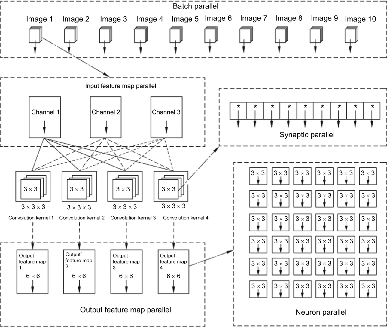
However, in practice, the size of the input image, the number of convolution kernels, and the number of processed images are all large. As such, given the computing resources and architecture design of hardware, it is not possible to achieve the theoretical maximum parallelism during execution. This same argument can be made for types of operations other than convolution. The limitations of Amdahl’s Law also apply to the acceleration ratio in real practice. At present, various accelerators on the market actually seek an optimal balance between the parallelisms of various dimensions based on specific application requirements.
1.3.5: Application example
AI has a wide range of applications in real life, and is commonly used in robotics, natural language processing, image recognition, and expert systems. A simple application example for beginners is handwritten number recognizing, which is equivalent to the “Hello World” program for beginners to learn programming. Handwritten numbers are widely used, and humans can understand handwritten numbers without difficulty, but for computers it is very challenging. In the early days, traditional methods were adopted. In order to program a computer to recognize handwritten numbers, it took a long time and the recognition accuracy was not high. While people were racking their brains regarding this problem, researchers found that it is easy to solve such problems through machine learning.
Turing Award winner LeCun first established a dataset known as MNIST (Modified NIST and MNIST) through the National Institute of Standards and Technology (NIST) handwritten digit library [8]. The MNIST dataset contains handwritten images of 70,000 Arabic numerals, as shown in Fig. 1.24. These digital images are grayscale and were collected from various places. The dataset is split such that 60,000 can be used as training data, and the remaining 10,000 are to be used as test data. The size of each picture is 28 × 28. Based on the MNIST dataset, researchers have proposed a variety of handwritten digit recognition networks, which have improved algorithm accuracy to a level comparable to humans.
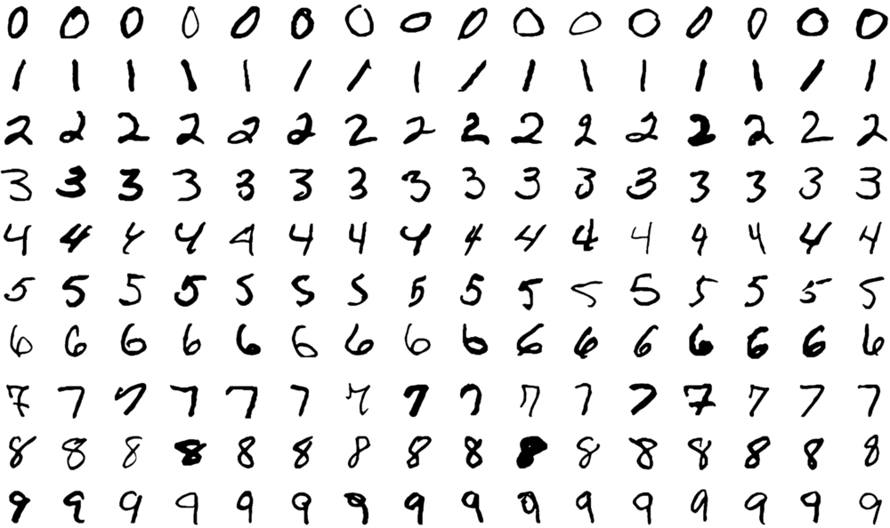
The MNIST dataset only includes numbers from 0 to 9. The task is to arbitrarily select a picture with a number and let the computer recognize it. From another angle, the task can be considered as classifying the digital meaning of the picture into one of 0–9. Let us take a clear look at the process of digit recognition.
This case is realized by a LeNet network, a CNN proposed by LeCun. The LeNet network is also one of the earliest CNNs. As shown in Fig. 1.25, a simple digit recognition process includes the steps of loading a dataset, constructing a neural network structure, initializing, training, and testing. The training includes two substeps: validation and tuning.
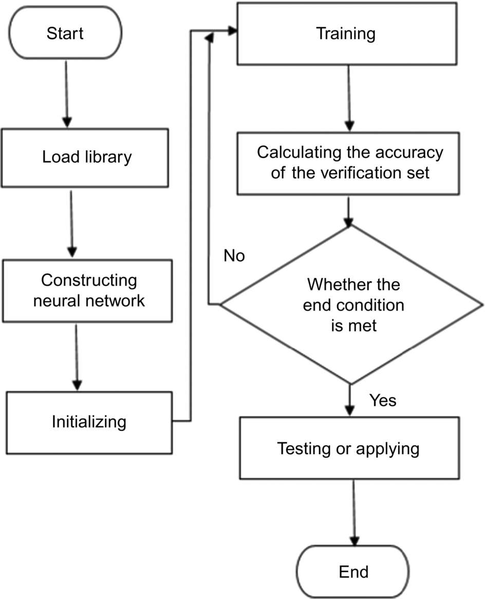
1.3.5.1: Initial setup
In the initial setup stage, loading datasets, constructing neural network structures, and initializing operations are needed. Usually the MNIST dataset needs to be loaded first for training and testing. Next, we need to construct a neural network, defining the corresponding input layer, convolution layers, downsampling layers, fully connected layers, output layer, and the connections between them. Moreover, the input and output dimensions of each layer must be specified. These aspects of the network structure are considered as hyperparameters. Except the first layer, which needs to be clearly specified, the input and output sizes of the hidden and output layers can be automatically inferred. Specific hyperparameters include the size of the convolution kernels in the convolution layer, the step size of the downsampling layer, and the number of nodes in the fully connected layer.
If the digit recognition program is to be trained on GPU, it is often necessary to allocate the GPU device and reference the upper limit of the memory occupancy. The setting of these parameters with different GPU hardware configurations is very important in determining how to use the resources of the GPU efficiently. The GPU should be allocated as needed so as to make the best use of the memory. Finally, when initializing, we need to set the trainable parameters such as the convolution kernels of convolution layers, weights and biases of fully connected layers, and assign initial values to these parameters based on the specified initialization methods (such as Gaussian random initialization, constant initialization, etc.).
1.3.5.2: Training
In the training stage, the data from the training dataset is transferred to the neural network, and the neural network attempts to learn the patterns exemplifying each class. The trainable parameters of the model are consistently modified to make the neural network converge. At the same time, we consistently calculate the accuracy of the current model on the validation dataset and decide whether the model has reached the required accuracy or whether there has been any overfitting. Generally, the training should be stopped when the number of training steps specified in advance has been reached, when the model has converged, or when the target accuracy has been reached. It is also possible that the parameters of the neural network have converged to a local optimum rather than the global optimum.
1.3.5.3: Test
As shown in Fig. 1.26, when testing the trained and optimized neural network, handwritten digits 2 and 7 are, respectively, fed into the handwritten input layer. After the neural network receives the test data, it carries out automatic prediction, and outputs the probability of each digit as the label of the input data. If the corresponding number is recognized, it will be displayed by the system. As shown in Fig. 1.26, the input images show the numbers 2 and 7, and the results of the corresponding output layer are highlighted with white squares.
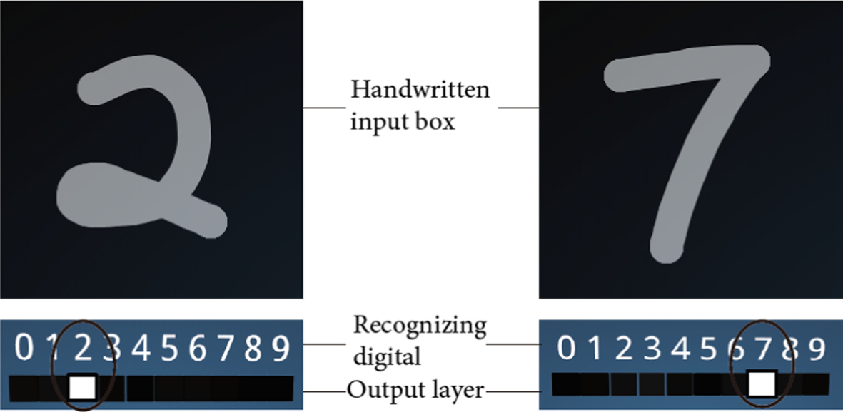
At present, handwritten digit recognition technology is quite mature and is mainly applied in the fields of large-scale data statistics, finance, taxation, and mail sorting systems. It greatly improves the recognition speed of digital numbers in specific businesses and has high application value.