
Chapter 6: Case studies
Abstract
This chapter focuses on the data and algorithms to run AI, based on the computation power of the Ascend AI processor. This chapter is divided into two sections. In the first section, the standard evaluation criteria for image classification and video-based object detection algorithms are introduced followed by the criteria to evaluate the hardware’s inferencing performance. In the second section, examples of image recognition and video object detection are used; their datasets and typical algorithms used, to illustrate how to develop customized operators and end-to-end applications on Ascend AI processors.
Keywords
Evaluation criteria; Accuracy; Mean average precision; Throughput and latency; Energy Efficiency Ratio; Image classification; Object detection; Model migration
The transformation of Artificial Intelligence (AI) from theoretical research to industrial practice depends on three factors: improvements in algorithms, computing power, and data. This chapter focuses on the data and algorithms to run AI, based on the computation power of the Ascend AI processor. This chapter is divided into two sections. In the first section, the standard evaluation criteria for image classification and video-based object detection algorithms are introduced followed by the criteria to evaluate the hardware’s inferencing performance. In the second section, examples of image recognition and video object detection are used; their datasets and typical algorithms used, to illustrate how to develop customized operators and end-to-end applications on Ascend AI processors.
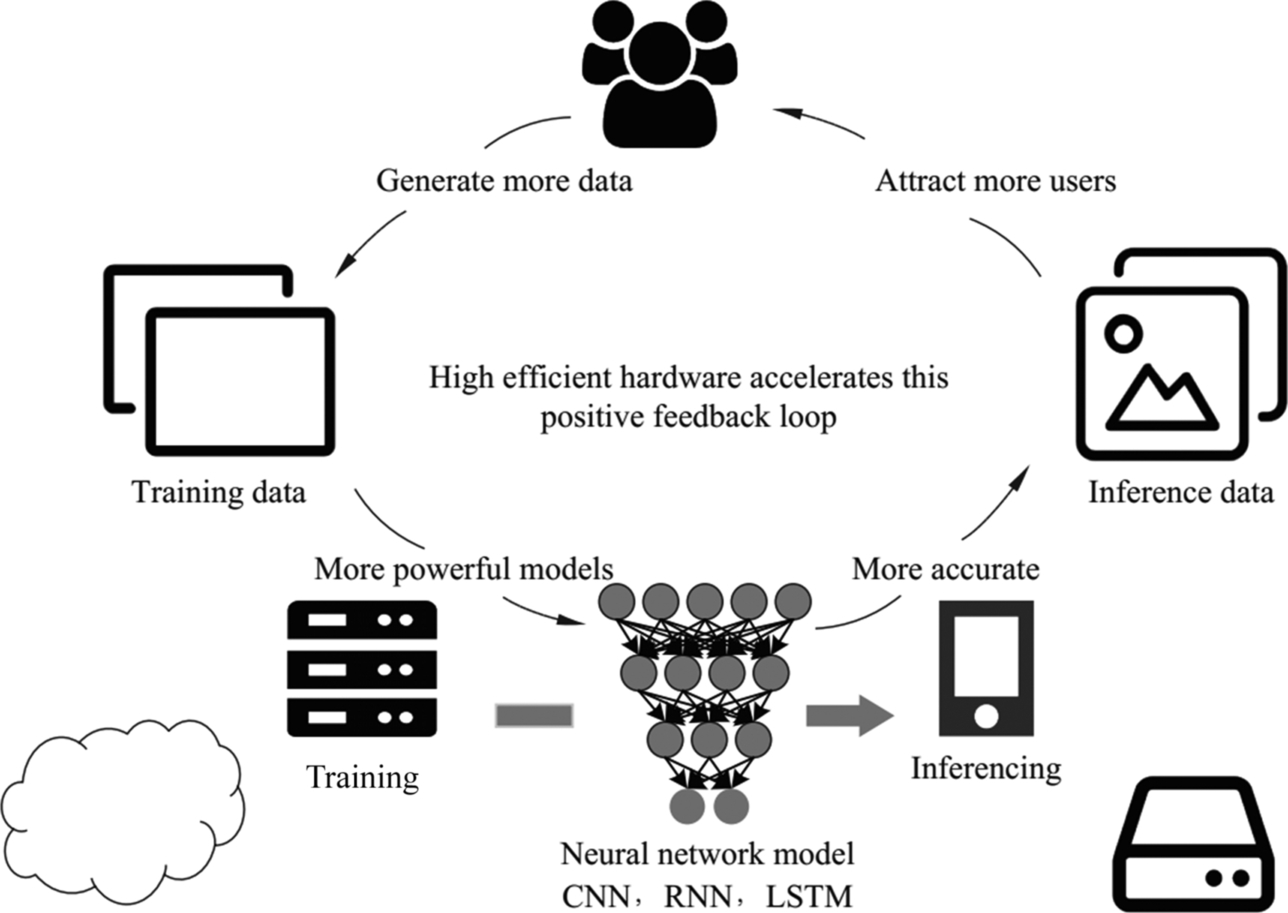
When considering machine learning as a storybook, there are two different storylines known as training and inference and the major characters of each differ slightly. The former is fulfilled by the algorithm scientists, the other is based on the work of algorithm engineers. As shown in Fig. 6.1, more users generate more data. To better characterize the data, algorithm scientists develop bigger models to improve accuracy. However, this causes the structure of the model to become more complicated, and as a result, more powerful training hardware is needed. As a result, more engineers work on deploying in richer scenarios, which attracts more users and generates more data. This series of “more” form a closed cycle in the research and application, which promotes the development of artificial intelligence.
Developers of artificial intelligence or algorithm scientists emphasize more on the training process. They design various complex or concise operators, training parameters, and fine-tuning hyperparameters of networks and verify the algorithm performance on given datasets. For the convolution operator, whose implementation has been introduced previously, as scientists are not satisfied with how it characterizes the data, a series of extended convolutions are proposed. For example, dilated convolution [1] can have a larger receptive field and deformable convolution [2] can describe the target object better with the same amount of weights.
Implementers of artificial intelligence focus more on the aspect of inference. A production-level system often requires real-time processing of dozens or even hundreds of HD images per second. For example, a company that specializes in video object detection for drones is unlikely to accept a network with hundreds of layers. A model with hundreds of megabytes and the electricity consumption of tens of watts are quite challenging for the weight-limited low-cost drones. Recently, more attention is given on researching algorithms that are more computationally efficient and require less memory. From MobileNet [3] to ShuffleNet [4], based on Group Convolution and Depth-wise Convolution, these compressed networks obtain a similar performance comparing to the original large networks such as GoogleNet and VGG16, with much fewer parameters and decreased model size.
For this reason, Huawei has launched the full-stack and full-scenario intelligent solutions from on-device (Fig. 6.2) to on-cloud (Fig. 6.3). From the perspective of technology, Huawei has a full-stack solution that includes IP and processor, processor enablement, training and inference frameworks, and application enablement. From the perspective of business, Huawei can provide services for full-scenario deployment environments including public and private cloud, edge computing, IoT, and consumer terminals.


To provide the computing power for AI, the Ascend processors are developed into five series including Max, Mini, Lite, Tiny, and Nano, to satisfy the diverse requirements of different scenarios. On the top of the hardware, a highly automated processor enablement software stack CANN is also provided, including the aforementioned offline model conversion tool, offline model running tool, and tensor boost engine, to help R&D workers fully utilize the computing power of the Ascend processor. At the same time, as a unified training and inference framework which can work on-device, on-edge, and on-cloud independently or collaboratively, Huawei’s MindSpore is very friendly to AI researchers, so that the performance of the model can be further improved. At the application layer, ModelArts, which can provide services for the entire pipeline, offers layered APIs and preintegrated solutions for users with different requirements.
As a typical inference processor, Ascend 310 takes the advantages of its low power consumption and high performance and targets at efficient on-device deep neural network inference. It aims to use a simple and complete toolchain to achieve efficient network implementation and migration, from automatic quantization to process layout. Due to space limitations, details on how to design a neural network will not be discussed in this book. More descriptions are focused on the support of Ascend AI processors for various networks, illustrating how to migrate appropriate networks to the Ascend development platform.
6.1: Evaluation criteria
This section will briefly introduce the standard evaluation criteria for image classification and video object detection (accuracy, precision, recall, F1 score, IoU, mean average precision, etc.), as well as for hardware (throughput, latency, energy efficiency ratio, etc.).
6.1.1: Accuracy
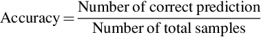
For classification problems, accuracy is an intuitive evaluation measure, which refers to the percentage of correctly classified samples in the total samples.
Let’s start with the following example:
A feasible solution for the classifier is to let {“yellow = apple” and “green = pear”}, which means that all yellow fruits are apples and all greens are pears. The shape of the fruits can be ignored at this moment because both fruits have the same shape (round) and hence this feature cannot differentiate between the two fruits.
The Accuracy of this classifier is:

It looks not bad, does it?
Next, let’s modify the data set slightly:
It seems that there are little changes from dataset1 to dataset2 as 90% of apples are yellow and 95% of pears are green. The only change is the number of each fruit. Accuracy for the same classifier, {“yellow = apple”, “green = pear”} is:

It doesn’t seem to be a problem, but what about creating a classifier based on shape, such as {“circle = apple”, “square = pear”}? The “square” attribute does not appear in the data. It can be replaced by any attribute that is not round, such as “triangle.” Then all round fruits are considered as apples, which also means all pears are classified as apples. Take a look at the performance of this classifier:

The classification based on shapes seems very unreasonable, since all fruits will be classified into one category, and this classifier is useless in a strict sense. However, based on the accuracy score as above, it seems much better than the classifier which is based on colors, and it is worth thinking about. In some applications, simply taking accuracy as the only evaluation measure may cause problems with serious consequences. Taking the earthquake prediction scenario as an extreme example, if a sample is taken every second, there will be 86,400 data points each day, and there is usually NO single positive sample for the nearly 2.6 million data points collected in a month. If the accuracy is taken as the measurement, the model will undoubtedly choose to classify the category of each test case into 0 (no earthquake) and achieve an accuracy of over 99.9999%. As a result, in the event of an earthquake, the model will not predict it correctly, resulting in huge losses. Researchers would like to choose to report false positives to capture such rare samples. The same situation applies to rare disease recognition tasks. It is better to give more tests to a suspected patient instead of failing to identify the rare disease.
The classification on a dataset with imbalanced data size of different categories is generally referred to as an imbalanced data classification problem. To evaluate this kind of problem better, some new evaluation concepts need to be introduced.
As shown in Table 6.1, if the prediction result is a pear (positive) and the ground-truth label is also a pear, then the prediction belongs to true positive (TP). If the predicted value is ‘pear’, but the real ground-truth value is ‘apple’, the prediction is false positive (FP). If the predicted value is apple (negative) and the ground-truth value is also apple, the prediction belongs to true negative (TN). If the predicted value is an apple, but the ground-truth value is a pear, the prediction is a false negative (FN).
Table 6.1
| Predictionground truth | Pears: Positive | Apples: Negative |
|---|---|---|
| Pears: Positive | True positive (TP) | False positive (FP) |
| Apples: Negative | False negative (FN) | True negative (TN) |
Based on the above description, we can give the definitions as:


The performance of the above classifier {“round” = apple, “square” = pear}, can be given as Table 6.2:

Table 6.2
| Predictionground truth | Pears: Positive | Apples: Negative |
|---|---|---|
| Pears: Positive | 0 | 0 |
| Apples: Negative | 100 | 10,000 |
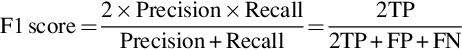
For this given problem, if precision and recall are used as evaluation metrics, the results of the shape classifier will not be misleading. For specific cases, evaluation criteria should be set reasonably in accordance with the data distribution and data characteristics. If the goal is to design a relatively balanced classifier, the F1 score is a good evaluation measure to use:
Once the evaluation criteria are determined, let’s look back to the original dataset. Can 200 fruits in the warehouse represent all the apples and pears? Are there other fruits? How many different colors are there for apples in the real world? What are their percentages? Will it misclassify red apples from yellow apricots? How about round oranges from star carambolas? The list goes on and on. Sufficient data collection and preparation is the prerequisite for the success of any intelligent model. With the increased capability of current AI models, existing algorithms can deal with more types of features, while the demand for data also increases as well. To train a high-performance model, it is essential to make the right assumption on scope and type of sampled data, based on the context of the actual task. Various data modeling details including overfitting and underfitting will not go into detail here due to space limitation. For those interested please read [5] by Ian Goodfellow, Bengio, and Aaron Courville, three pioneers of deep learning.
To summarize, the accuracy metric does not consider the objective of the classification, since it only focuses on calculating the percentage of correct predictions on each category. The use of accuracy as an evaluation measure should be with great caution, especially for classification tasks, in which the data has imbalanced categories. On the contrary, precision, recall, and F1 score are practical evaluation measures for real applications, and the selection of the evaluation measure for the classifier should be based on the data and label characteristics of the actual cases.
6.1.2: IoU
Based on image classification, a series of more complex tasks can be extended according to different application scenarios, such as object detection, object localization, image segmentation, etc. Object detection is a practical and challenging computer vision task, which can be regarded as a combination of image classification and localization. Given an image, the object detection system should be able to identify the objects in the image and provide their location. Comparing to image classification tasks, as the number of objects in an image is uncertain and the accurate location of each object should also be provided, the task of object detection is more complex and its evaluation criteria are more controversial.
As shown in Fig. 6.4, an object detection system can output several rectangular boxes and labels. Each rectangular box represents the boundary of the predicted object, as well as its category and position information. Both of these outputs are needed to be evaluated by developers. To evaluate the accuracy of the predicted boundary, the Intersection over Union (IoU) metric is introduced. To evaluate the correctness of the predicted category labels, the mean Average Precision (mAP) metric is introduced.
The concept of IoU is very intuitive; it illustrates the intersection of the predicted boundary and the ground-truth boundary. The bigger the IoU is, the higher is the performance of the prediction. If both intersections overlap entirely, the result is perfect.

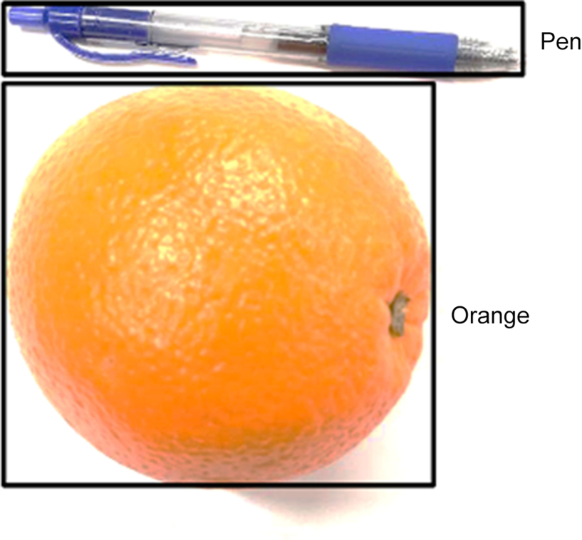
In Fig. 6.5, a solid border indicates the ground-truth boundary of the object “orange” and a dashed border indicates the predicted boundary. In general, a matrix can be defined with the coordinates of the upper left corner and the lower right corner of the matrix, namely:

The concept of IoU is not difficult to understand, but how is it calculated? Will the relative position between the predicated boundary and the ground-truth boundary affect the calculation? Should we discuss whether the two boundaries intersect on a case by case basis? Do any intersections contain the cases of nested overlap?
At first glance, it seems that it is necessary to discuss the relative positions and intersection types of the predicted boundary and the ground-truth boundary case by case and make decisions based on various coordinates situations. However, the calculation of IoU is not so complicated. For calculating the intersection, the position of the predicted border and the ground-truth border can be swapped arbitrarily, and the coordinates of the intersected bounding box of the two borders need to be calculated only. If the two borders do not intersect, the output of IoU must be zero.
Code 6.1 is the code for calculating the IoU. Take the top left corner of the image as the origin (0,0), and let the x-axis extends to the right and the y-axis extends downward. The input parameters are the coordinates of the upper left and lower right corners of the predicted and the ground-truth borders. The output IoU score is a floating-point number between [0,1]. Assuming that the overlapping area of the two borders in Fig. 6.5 is the case of inter, the x coordinate inter_xmin of the upper left corner is the min value between {xp1 and xt1}, and the y coordinate inter_ymin is the max one between {yp1 and yt1}. Similarly, we can get the x and y coordinates (inter_xmax, inter_ymax) of the lower right corner. Worth noting here is that if the borders do not overlap at all, the value of inter_xmax - inter_xmin may be negative, which needs to be set to zero using the np.maximum function as Code 6.1. If either of the x and y axis does not overlap, the predicted and ground-truth borders do not overlap. The area of the intersection between the predicted border and the ground-truth border can be calculated using the coordinates of the inserted points on the diagonal direction. The area of the union can be obtained by adding the area of the two borders. Then the IoU ratio can be obtained by dividing the intersection area by the union area.
If you are interested, you can build your own sample to test it. In actual programming, it is common to add 1 to the length and width when calculating the area.
6.1.3: Mean average precision
As the name implies, mean Average Precision (mAP) refers to the mean value of the average precision of each category. The average precision here refers to the area under the Precision-Recall curve (PR curve).
For most algorithms, given a data sample, the prediction of a model is based on its derived confidence value between [0, 1]. If the confidence is higher than a threshold, the corresponding sample will be classified as positive, otherwise negative. It is obvious that the threshold value directly affects the results of prediction. In practice, precision and recall of the model can be controlled by adjusting the threshold. Generally, a higher precision will result in a lower recall or vice versa. Briefly, precision indicates the percentage of true positives in the predicted positives, and recall shows what percentage of the ground-truth positives is predicted as positive. Different tasks have different preferences for precision and recall. Efforts are often made to improve the performance on one of precision and recall without sacrificing the other. For example, given a requirement of at least 70% of ground-truth positives to be detected, it allows improving the precision as much as possible while keeping the recall value not lower than 0.7.
The precision-recall curve can be drawn intuitively as Fig. 6.6,a where the vertical axis P represents the precision and the horizontal axis R represents the recall. It is easy to draw a typical precision-recall curve using the automatically generated classification data from sklearn. When recall increases, the precision decreases gradually. In practice, it is usually difficult to calculate the accurate area under the PR curve. Usually, the approximate average precision is computed by changing the value of recall from 0 to 1 gradually with a fixed step size (e.g., 0.01).

In the problem of object detection, the mAP is often used as a unified indicator for considering the two kinds of errors from precision and recall. Because of the special requirement for object detection, the IoU is used to determine whether an object of a particular category is accurately detected or not. The value of the threshold can be set based on the actual applications. The typical threshold value is usually 0.5. In practice, a detection model may output multiple predicted boundaries (more than the number of ground-truth boundaries) for each image. If the IoU of the predicted and ground-truth bounding boxes is larger than 0.5, the predicted bounding box is considered to be correct, otherwise, the predicted bounding box is considered to be wrong. With more bounding boxes predicted, the recall increases as well. By averaging the precision at different recall rates, the corresponding average precision value can be obtained. The final mean average precision can be obtained by computing the mean value of the average precision of all object classes.
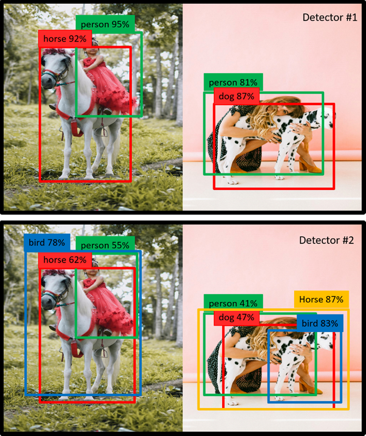
One problem that can be easily ignored is how to set the threshold of the IoU when calculating the mAP. If the threshold is set too low, even the erroneous bounding box detections can get excellent scores. As shown in Fig. 6.7, we designed two object detectors, both of which are considered to perform perfect predictions of the object boundary under the measurement of mAP, while the performance of detector 2 was actually far from the ground-truth label. In the article “Best of both worlds: human-machine collaboration for object annotation”, it is also mentioned that it is actually difficult for human eyes to distinguish the object boundary corresponding to IoU = 0.3 and IoU = 0.5. Needless to say, this situation may cause some problems in the development of practical applications. The ways to evaluate object detectors can vary from each other, depending on the context of the actual application. In practice, the average precision corresponding to different IoU thresholds (0.5–0.95, with 0.05 as the step size) is often calculated. With further average computation, the average precision of objects of different sizes also can be obtained. This is how the object detector is evaluated on the MS COCO dataset [6] in the following section.
6.1.4: Throughput and latency
The training process usually involves massive training data and complex neural networks. To train the parameters in the model, it requires a huge amount of computation and the processor requirements are quite high in terms of computing power, accuracy, and expansibility. The inference process involves testing the trained models on new data. For example, a video monitoring device determines whether a captured face is suspicious based on the backend deep neural network model. Although the inference process has much fewer operations than training, it still involves a lot of matrix operations.
During training, accuracy is more critical, while performance such as real-time and speed are more important during inference. Throughput is one of the easiest measures to evaluate the overall performance of inference, i.e., the number of images that can be processed per second when running a model. Latency (reciprocal of the throughput) is the average time spent to infer each image and is one of the important metrics to measure performance. Generally, the unit of latency is milliseconds (ms) and the time used to process the first frame is often excluded when calculating the average latency. The throughput can be computed by dividing 1000 (number of milliseconds per second) by the latency.

As mentioned previously, the computing power of a processor is commonly measured by TOPS, which is the number of operating basic deep learning operators per second. If the computing power of a processor is used as a measurement for hardware, throughput is the performance measurement based on the integration of hardware and software. It is highly related to the data structure, model architecture, and even the batch size for batch processing. In general, given data with the same type and size, the model which has fewer parameters has a faster absolute processing speed and higher throughput. Of course, as the complexity and number of parameters of the deep learning model increase, it shows more advantages of the high computing power and low energy consumption of specialized processors such as the Ascend AI processor.
It is important to note that the operands defined in a processor may vary depending on the type and precision of the computation, which will result in different throughput. Therefore, when stating the performance of a processor (including computing power, energy efficiency ratio, throughput, etc.), some detailed information, such as the computing type and precision (such as FP16 or INT8), should be provided. Sometimes the neural network architecture of the computational model should also be provided to facilitate a relatively fair comparison. By quantization, the model trained with FP32 precision can be compressed into FP16 or INT8 version for inference. Typically, the lower the data quantization precision is, the worse is the accuracy of the inference. A proper quantization technique can improve throughput while avoiding the loss of precision for inference.
6.1.5: Energy efficiency ratio
The unit of the energy efficiency ratio is TFLOPS/W, which is defined as average computing power when the processor consumes 1-Watt electricity power. In practice, given the precision, batch size, model architecture, and data characteristics, Watt/Image is also often used to measure the average power consumption per image.
As mentioned previously, the higher the TFLOPS is, the faster is the processor and therefore, theoretically, the processor can provide a larger throughput with the same algorithm and data. However, in engineering practices, larger throughput is not always the best choice. The selection of computing power should be based on the context of the practical application. Taking the power of the light bulbs as an example, a bulb is often brighter if it has a larger watt. However, there is no need for 300 W searchlights everywhere, and the high-watt bulb will not even glow if the local power system is not strong enough. The choice of light bulbs is limited by the power supply and environment, so as the choice of artificial intelligence processors.
The application scenarios of AI are rather complicated. To achieve the same computing power, the electricity power consumed may vary due to different processor architectures or different model structures. Meanwhile, more advanced deep learning models usually work with more parameters, and hence the requirement for computing power is higher. Although companies can design processors with different computing power for different scenarios, it is definitely more desirable to achieve a higher computing power for the same application scenario or with the same power consumption limit.
With the recent rapid development of deep learning, the vast energy consumption of data computation has attracted more and more attention. To save energy costs, Facebook chose to build its data center in Sweden, not far from the Arctic Circle. The average winter temperature there is about − 20°C, and cold air enters the central building and naturally cools the servers by exchanging with the generated hot air. Subsequently, a joint venture between the United States and Norway, Kolos, also proposed to construct the world’s largest data center in the Norwegian town of Barnes, which also located in the Arctic Circle. The power consumption of this proposed data center is 70 MW, with 1000 MW as its peak value.
On average, training a deep learning model produces 284 tons of carbon emissions, which is equivalent to one-year carbon emissions of 5 vehicles. Therefore, the energy efficiency ratio becomes more and more critical when evaluating the deep learning platform. The design of the dedicated neural network processors can be customized based on the algorithm to reduce excessive power consumption and improve the computation efficiency. With improved performance, these processors will have a bright future in applications on mobile devices, which require high-performance and low energy consumption.
6.2: Image classification
Considering the maturity of deep neural networks in computer vision, this chapter explains how to create a typical application with Ascend AI processor using image classification and video object detection as examples. In the image classification example, a command-line-based end-to-end development pipeline is explained, and the model quantification method is also briefly introduced. The video object detection example focuses on how to customize the operators in the network and then discusses the factors that affect the performance of inference.
6.2.1: Dataset: ImageNet
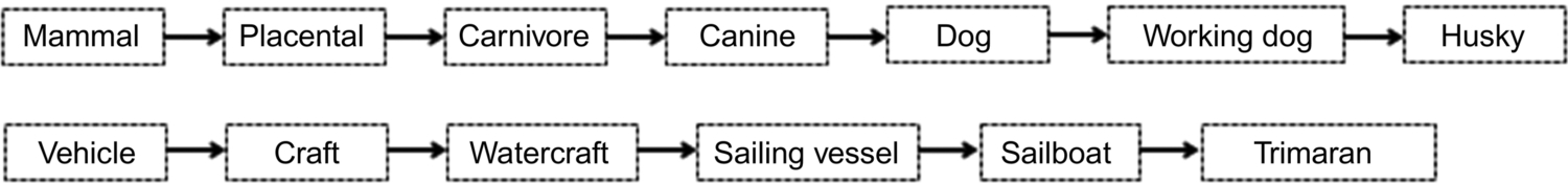
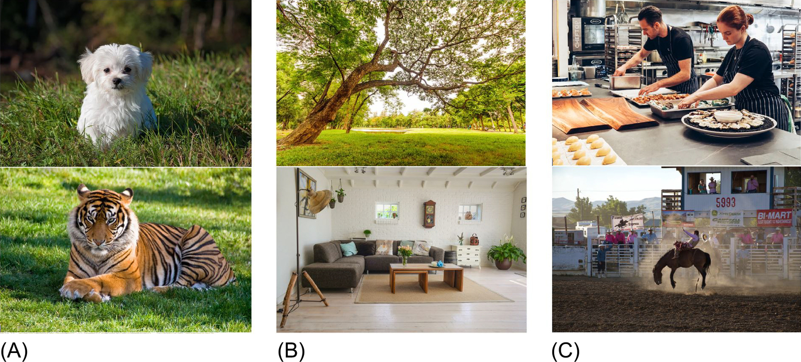
In this chapter, the ImageNet dataset [7] is selected for image classification because of its richness of data composition and its popularity in computer vision. Being the largest image dataset in the world now, it has about 15 M images covering more than 20,000 categories. It is also known as the first dataset that is annotated based on the WordNet semantic hierarchy. As in Fig. 6.8, the semantic hierarchy of ImageNet from top to bottom level is shown from left to right. For example, “husky” is a subset of the “working dog,” “working dog” is a subset of the “dog,” “dog” is a subset of the “canine,” “canine” is a subset of to the “carnivore,” and “carnivore” belongs to “placental” which is a subset of “mammal.” Although there are ambiguous labels in ImageNet dataset at some levels, it is much better than other datasets in which “female” and “human” are classified into completely distinct categories. The directed acyclic semantic structure itself provides a good reference for extracting the semantic feature from various images. At the same time, the tree-structure organization also facilitates researchers to extract the desired information and select certain specific nodes to train the classifier based on their application needs. It can be imagined that the features that distinguish “cats” from “dogs” are not the same as those features which distinguish “trucks” from “cars.”
There are three types of tasks defined on ImageNet: image classification, single object detection, and multiple object detection. The most popular one is image classification, in which the model only needs to classify the object in the image into a particular predefined category. Most images of this task come from Flickr and other search engines. Each image was manually labeled into one of 1000 categories, and each image is supposed to have just one object of a particular category. The number of images for each category may be from one to several, and their sizes and shapes may vary as well. In the paper, “ImageNet Large Scale Visual Recognition Challenge” [8], the authors summarize the ImageNet dataset from eight dimensions, including scale, the number of instances, texture type, etc., ensuring the diverse and representativeness of the dataset. At the same time, the granularity of categories of ImageNet is finer than that of a similar dataset PASCAL [9]. The class of “birds” in the PASCAL dataset will be subdivided into several categories including flamingo, cock, ruffed grouse, quail, and partridge in ImageNet (Fig. 6.9). It is worth mentioning that this type of fine-grained classification also causes difficulties for people who do not have sufficient prior knowledge. The human classification error rate on the dataset reached 5.1%, partly because the image quality is low and the target object is not prominent. Some volunteers gave feedbacks that they labeled incorrectly because they could not accurately classify “quail” from “partridge”, both of which are not popular birds. To some extent, this is one of the reasons why the classification accuracy of the recent models on ImageNet is higher than that of humans, while it still cannot prove that machine learning is more intelligent than a human.

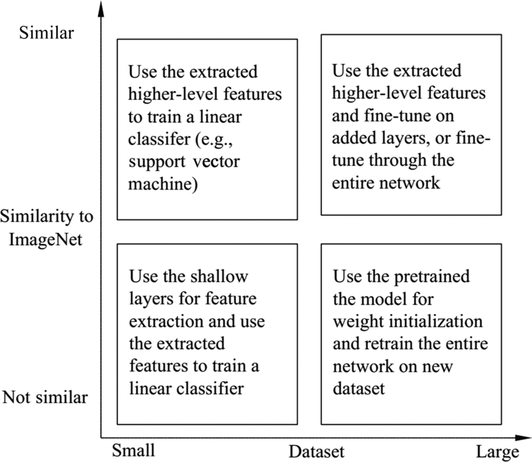
Along with the birth and development of ImageNet, the world-famous “ImageNet Large Scale Visual Recognition Challenge (ILSVRC)” [7] began in 2010. In the competition, two evaluation measures are used: Top-1 error rate (for a certain image, whether the label with top one probability predicted by the algorithm is the same to the ground-truth label) and Top-5 error rate (whether the labels with top five probabilities predicted by the algorithm is the same as the ground-truth label). In 2012, AlexNet, the winner of ILSVRC competition, marked the first time that the convolutional neural network is able to classify with a top-5 error rate of 15.4%, while the top-5 error rate of the second-ranked model is 26.2%. The whole community of computer vision was shocked by the performance and deep learning became popular since then. GoogleNet and VGGNet in 2014 and ResNet in 2015 are subsequent impressive models because of their great achievements. Since then, “model trained on ImageNet” means that the model is trained and evaluated on the data provided by a particular year of ILSVRC (the data of ILSVRC 2012 is most commonly used). At the same time, researchers are surprised to find that the model trained on ImageNet (pretrained model) can be used as the basis for fine-tuning parameters of other image classification tasks, which is especially useful when the training data is insufficient. By using the intermediate result of a specific layer before the fully connected layer, this first part of the model can become an excellent image feature extractor. The second part of the model can be designed based on the requirement of the application. After fine tuning with a certain amount of data, a good result can usually be obtained. Fig. 6.10 briefly summarizes some suggestions for using the pretrained model and transfer learning for image classification, w.r.t. the data size of the target application, and its similarity to ImageNet.
When looking back, ImageNet was only published as a poster at a corner of CVPR2009. While 10 years later, in CVPR2019, it won the “PAMI Longuet-Higgins Prize,” which shows its significant contribution to computer vision research. Many people regard ImageNet challenge as a catalyst for the current wave of artificial intelligence, and the participating companies from various areas of the tech industry spread all over the world. From 2010 to 2017, in just several years, the classification rate of the winners increased from 71.8% to 97.3%, which has surpassed the performance of a human. It also demonstrates that more data can lead to better learning results. “ImageNet has changed people’s understanding of datasets in the field of artificial intelligence. People begin to realize that datasets are as important as algorithms in research”, said by Professor Fei-Fei Li from Stanford University.
6.2.2: Algorithm: ResNet18
The key to deep learning is probably the “deep” layers. The technique that transforms networks from two or three dozens of layers, such as the VGG and GoogleNet, to hundreds of layers is the residual block. As one of the top performed networks for image classification on ImageNet dataset, Deep Residual Net (ResNet) ranked first place in ILSVRC 2015. It outperformed the second-ranked system with a big gap in all three tasks of image classification, object detection, and object localization. Their top-5 error rate was as low as 3.57%, which refreshed the record of precision of CNNs on ImageNet. The residual block, proposed by Kaiming He et al., provided a solution to resolve the difficulties of training networks with deep structures, and it became a milestone in the history of deep learning.
To understand ResNet, let us first look at the Degradation problem is solved. Degradation is the phenomenon that the performance of the neural network decreases while the number of layers increases. Generally speaking, for the deep learning networks with convolutional layers, theoretically, with the increasing number of network layers, there should be richer feature extraction and the accuracy of the network should increase as well. However, when the number of network layers reaches a certain level, its performance will be saturated, and further adding new layers will lead to a degraded of the overall performance. Surprisingly, this degradation is not due to overfitting, because the performance decline on both the test and the training set, which differs from the obvious characteristics of overfitting, i.e., the performance decreases on the test while the performance increases on the training set.
To some extent, this is even counterintuitive—how could a deeper network be less effective than a shallow one? In the worst case, the later layer only needs to make an identity mapping for the incoming signal, i.e., the output signal of the previous layer does not change after flowing through the current layer, and the error rate after the information passing through current layer should be equal. In the actual training process, due to the limitations of the optimizer (such as stochastic gradient descent) and data, the convolution kernel is difficult to converge to the impulse signal, which means the convolutional layer is actually difficult to achieve the identity mapping. Therefore, the model cannot converge to the theoretical optimal result after the network depth becomes deeper. Although the Batch Normalization technique can solve a part of the gradient loss problem caused by back propagation, the problem of network performance degradation with increased depth still exists and it has become one of the bottlenecks that restrict the performance of deep learning.
In order to solve this problem, ResNet proposed the residual block (Fig. 6.11b). Given input as x, the goal to learn a mapping H(x) as the output of the neural networks. In the figure, F(x) is the learned mapping from the weight layer. In addition to the output of the weight layer, another connection directly connects x to the output. The final output is obtained by adding x to F(x), which uses the entire residual block to fit the mapping:

It is easy to see that if F(x) is zero (i.e., all parameters in the weight layer are zero), then H(x) is the identity mapping, as mentioned above. By adding the Shortcut structure, the residual block provides a way for the network to converge to identity mapping quickly and tries to solve the problem of performance degradation when the depth goes deeper. This simple idea really provides a solution for the difficult problem of fitting identical mapping using convolutional layers, which makes it easy for the optimizer to find the perturbations on the identical mapping instead of learning the mapping as a new function. Because of these characteristics, ResNet achieves an outstanding performance on various computer vision datasets, including ImageNet.
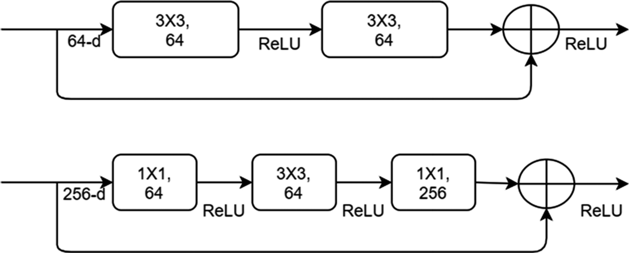
To illustrate the performance of residual networks with different depths, the author designed 18-, 34-, 50-, 101-, and 152-layer residual networks, respectively. In practice, ResNetN is often used to represent n-layer residual networks. In order to reduce the number of parameters and computation, when using deeper networks, the high-dimensional input, e.g., 256 dimensions, is first reduced to 64 using 1 × 1 convolution, and to use 1 × 1 convolution to recover back afterward. The details are shown in Fig. 6.12, and the top figure is a residual block of ResNet18/34, and the bottom is the residual block of ResNet50/101/152, which is also called as a Bottleneck Design. It is a good practice to compare the difference of parameters numbers between residual block with bottleneck design and conventional residual block.
Experiments show that the residual network can effectively solve the problem of performance degradation when the depth goes deeper. In general, a conventional CNN suffers the aforementioned degradation issue, however, with residual network architecture, the performance continues to be improved along with the depth of the network, i.e., a 34-layer version consistently outperforms than its 18-layer counterpart in both training and validation set.
It is easy to get the implementation of the residual network on the official website of TensorFlow [11]. To note here is that the description in this chapter is based on the publication “Deep Residual Learning for Image Recognition” [10] in 2015 and it corresponds to the v1 version of TensorFlow’s official implementation. The author, Kaiming He, in the following year (2016) published another article “Identity Mappings in Deep Residual Networks” [12], and it includes details about the relative positions of activation function and batch normalization which are ignored here. The corresponding code is available as v2 version of the implementation.
6.2.3: Model migration practice
The Ascend AI processor provides two ways to migrate trained models onto the processor. One is the integrated development environment, Mind Studio, and the other is the digital developer suite. Both methods are based on the same set of artificial intelligence full-stack development platforms developed by Huawei. The former provides the drag-and-drop style visual programming, which is suitable for the beginners for a quick start. The latter offers a command-line development suite, which is suitable for advanced developers for customized development.
This section takes the reader through the deployment process of applications on the Ascend AI platform using the command line (DDK). The reader is supposed to finish the installation of the DDK (for details on installation, see “Ascend 310 DDK sample usage guide (command mode)” or “Ascend 310 Mind Studio installation guide”), and the DDK installation directory is $HOME/tools/che/DDK, where $HOME represents the user’s home directory.
Generally, several steps are involved to migrate a model. This section will introduce each of them:
- • Model preparation: Get the model weight file and convert it into the DaVinci offline model file which is supported by Ascend AI Processor.
- • Image processing: Process images using DVPP/AIPP for decoding, cropping, etc.
- • Project compilation and execution: Modify the configuration file, set the install folder for DDK, path to the model file, and runtime environment parameters and compile the code to the executable file.
- • Result verification: Verify the inference result of the model.
6.2.3.1: Model preparation
We assume that the network has been trained on the host side and the corresponding weight file has been computed. For this example, you can download the trained weight file from the home page of Kaiming He,c the main contributor to ResNet. As mentioned above, a residual network has implementations for different depths. The provided link contains models for ResNet-50, ResNet-101, ResNet-152, etc., with their corresponding weight file (caffemodel) and prototxt file. Here, the 50-layer ResNet50 is used as an example.
Interested readers can learn about the operators and network structure of ResNet from its configuration document, such as prototxt/ResNet-50-deploy.prototxt. For example, Code 6.2 prototxt defines the input parameters for this sample case, and it shows that the input data is a three-channel image with a size of 224*224 pixels. The reader can prepare the test data according to the input parameters in this file.
To understand the configuration of specific layer in the neural network, the convolutional layer in Code 6.3 can be used as an example.
Based on what you have learned in the previous chapters of this book, it is easy to see that “bottom” refers to the input of the current layer and “top” is the output of the current layer. The “type” indicates the characteristics of the current layer and the value “Convolution” here means the current layer is a convolutional layer. The field “name” refers to the name of the current layer and is free to be defined by the reader, but note that this name is used as a reference to the relative position of the layer in the network, so this value needs to be unique.
Next comes the parameter setting for the convolutional layer, which has 64 convolution kernels (the “num_output” field in the code) of size 7*7 (i.e., the “kernel_size” field in the code). The field “pad” refers to the amount of padding at image edges, and the default value is 0, which means no padding. The padding needs to be symmetric in the up, down, left, and right directions. Here, the size of the convolution kernel is 7*7, as shown in the following Fig. 6.13 (nonreal pixel ratio). The number 3 here means that all 4 edges of the image have been expanded with (7–1)/2 = 3 pixels to extract features from the pixels at the image edge successfully. The field “stride” refers to the step length of the convolution kernel, whose default value is 1. Here, the stride value is set to 2, i.e., the convolution is calculated every two pixels; stride_h and stride_w can also be used to set the vertical and horizontal stride values, respectively.

When the model file is ready, it needs to be converted into the offline model file supported by the Ascend AI processor. During the process of model migration, any unsupported operators are required to be customized by the user themselves. The customized operators can be added to the operator library to make it possible for the model migration. The process for customizing operators will be introduced in the following section, the implementation of object detection, in detail. All operators of ResNet, in this section, are supported by the built-in framework of the Ascend AI platform. The user can directly migrate the model using the following commands (Code 6.4). After executing the command, a model file with the extension .om is generated, e.g., the resnet50.om file.
Here:
- • model: relative path to the model configuration file resnet50.prototxt
- • weight: relative path to the weight file resnet50.caffemodel
- • framework: the type of backend framework
- – 0:Caffe
- – 3:Tensorflow
- • output: name of the output model file, defined by the user
6.2.3.2: Image processing
With the development of IoT technology, the demand for on-device image processing of edge computing has increased. Hence, the required number of image frames to be processed per second and the number of codec operations increased as well. To speed up image data processing, a DVPP module, which is dedicated to image processing, is provided on the Ascend AI platform. Taking Ascend 310 as an example, its dual-core VDEC can process real-time dual-channel 4 K HD video at 60 frames per second, and its 4-core VPC can speed up to 90 frames per second, for real-time 4-channel 4 K HD video. With a higher compression rate such as H.264/H.265 and a large amount of computation for the codec, implementing the encoding and decoding operations on the hardware can effectively release CPU resources, so that data can be processed efficiently on the device.
In order to better represent and store images, the DVPP module supports two image formats including YUV and RGB/RGBA. As shown in Fig. 6.14, the YUV format is divided into three components. “Y” refers to Luminance or Luma, namely the gray value. “U” and “V” represent Chrominance, or Chroma, which describes the color saturation of an image, i.e., the pixel colors. The mainstream YUV formats are YUV444 (each pixel has Y, U, V values), YUV422 (each pixel has a Y value and two pixels share the same U, V values), YUV420 (each pixel has a Y value and four pixels share the same U, V values), and YUV400 (only Y value, i.e., black or white). The RGB format is more familiar to us, which can produce a wide variety of colors by changing the channels of red (R), green (G), and blue (B) and combining them with each other. The A in RGBA represents Alpha (transparency). RGB/RGBA format is defined according to the color identified by human eyes, which can represent most colors and is a friendly way to display on the hardware side, but it requires higher storage and transmission costs than YUV.

In this example, the preprocessing of images is already supported internally by the framework. Users can also call DVPP for image processing according to actual needs. There are mainly two methods to call DVPP, which are calling through the interface and calling through the executor. Due to the space limitation of this book, please refer to the attachment “Ascend 310 DVPP API reference” for detail.
6.2.3.3: Project compilation
In the local DDK installation directory, you can find a folder named sample, which contains a series of development cases for Ascend AI processors. Due to factors such as version upgrade and algorithm iteration, you are advised to obtain the reference samples of the classification network from the Ascend official website.c For typical scenarios such as image classification and object recognition, the corresponding code can be found there. Here, ResNet50 belongs to the image classification model. After the model conversion is done, you can start the local project compilation and execution based on the built-in image classification reference samples (classify_net/).
Considering that the context of the compilation environment is different, the compilation procedure is divided into two steps. It is recommended that the executable file and the dynamic link library file on the device side should be compiled separately. For the Atlas development board which is a computation platform with the independent processor for executing the inference, the environment for compiling executable files is on the device side. For the environment where the PCIe card or accelerator card is controlled by the central processing unit on the host side, the environment for compiling executable files should be set on the host side. For all types of Ascend platforms, the environment for compiling the link library and the scenario where the project is running should be consistent with itself.
Modify the “classify_net/Makefile_main” file according to the actual situation and compile the executable file. Modify the following items:
- DDK_HOME: ddk installation directory. The default value is “../../che/ddk/ddk/”.
- CC_SIDE: Indicates the side where the file is compiled. The default value is host. When the Atlas development board is used, set this parameter to device. Note that the value is in lowercase.
- CC_PATTERN: Indicate the scenario where the project is running, the default value is ASIC. In the Atlas scenario, the value is changed to Atlas.
After the modification, run the “classify_net/Makefile_main” file. You can generate a series of executable files in the “out” folder of the current path. The differences may vary depending on the software version and scenario of the reference samples. Modify the “classify_net/Makefile_device” filed to change the value of CC_PATTERN. The default value is ASIC. In the Atlas scenario, the value is changed to Atlas. After the execution is successful, a series of link library files including libai_engine.so are generated in the “classify_net/out” folder. So far, all the files required to execute the inference on the Ascend platform are ready.
After the compilation is completed, insert the ResNet50.om and ResNet50.prototxt that are successfully converted in the previous step into the “classify_net/model” path on the device side, and modify the corresponding path of the inference engine in “graph_sample.txt” according to the path described in the previous chapter.
The code in Code 6.5 is a typical sample of the basic definition of the inference engine. In the code, “id” indicates the ID of the current engine, “engine_name” can be determined by the reader, and “side” indicates the position where the program is executed (DEVICE indicates the device side and HOST indicates the host side). “so_name” refers to the dynamic link library file generated in the previous step. In “ai_config”, you can use the “model_path” field to configure the path of the model. In this example, the path is changed to the om path generated by the conversion.
6.2.3.4: Analysis of results
Based on the abovementioned evaluation criteria in this chapter, it is easy to know that the dataset commonly used by the ImageNet 2012 has 1000 class labels in the image classification task, and the prediction result provided by the model is also a 1000-dimension vector. As shown below, each horizontal row represents one dimension in the label vector. The first column indicates the ID of the corresponding label, and the second column indicates the probability that the label is true.
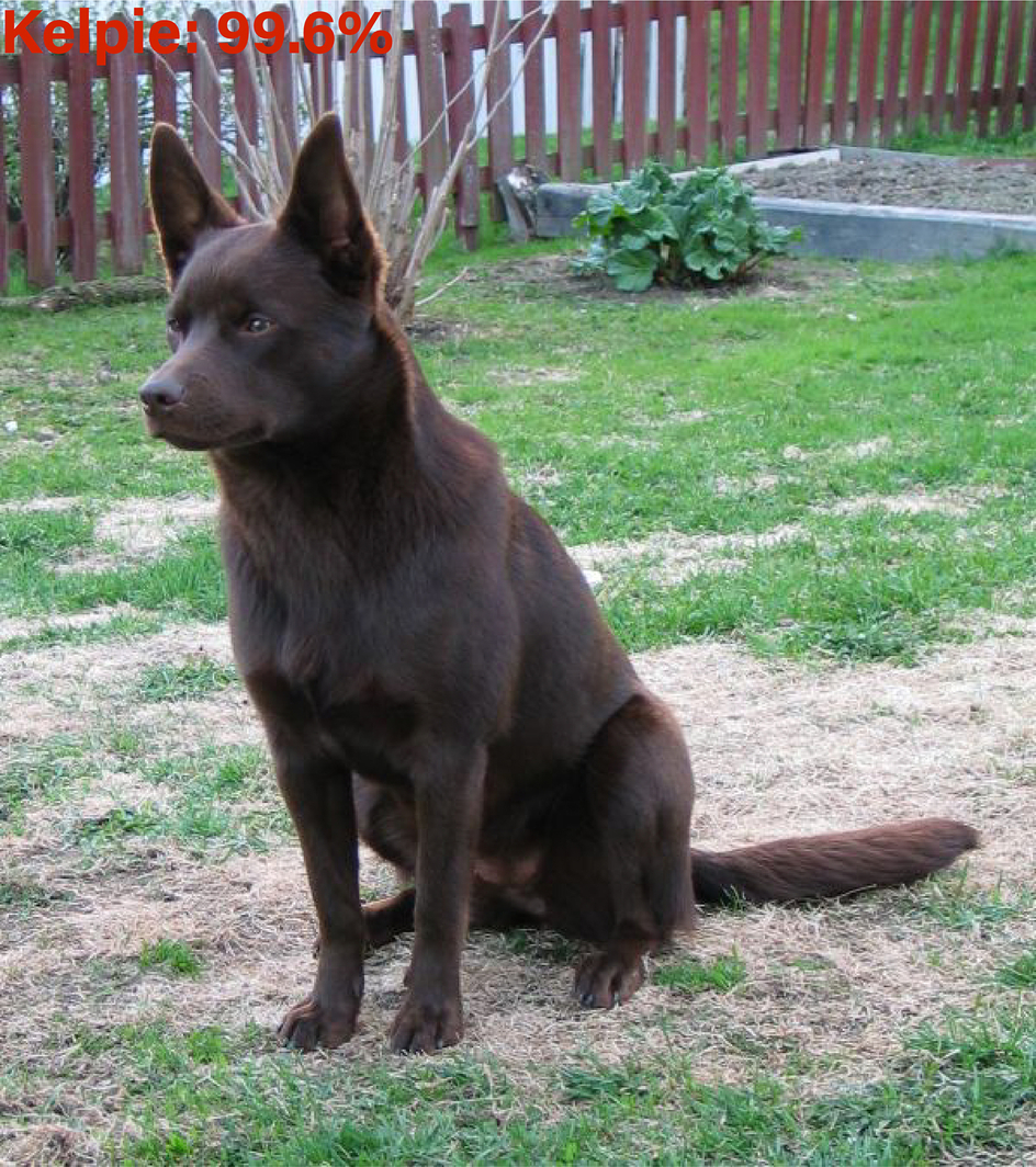
Generally speaking, the Top-1 prediction selects that the label with the highest value as the output label. The image input here is the Australian Kelpie dog, which is predicted accurately with the confidence of 99.8%. If you select MindStudio as the integrated development environment, which has built-in visualization function, you can right-click the resulting engine to view the result shown in Fig. 6.15.
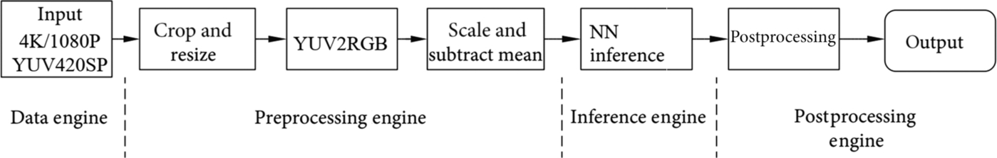
Finally, let us take a look at the pipeline of processing the input image by the Ascend AI processor in this case. As shown in Fig. 6.16, the DVPP module completes image transcoding, segmentation, and deformation. Next, the AIPP completes a series of preprocessing, including regularization, for input data. The DaVinci architecture processing core, which is the AI Core, processes the core inference. The operation result is sent to the CPU for postprocessing, and the postprocessing result is the output. The implementation and execution sequence of operators has been completed on the host side. You only need to perform offline inference calculations on the device side.
In the evaluation criteria section, the FP32 model is often quantified to FP16 or even INT8 precision in order to provide higher throughput and reduce the cost of energy consumption per image. The following section uses the residual network as an example to describe the general algorithm and performance of the quantization.
6.2.3.5: Quantification methodology
Compared with the FP32 type, the low-precision types such as FP16 and INT8 occupy less space. Therefore, the corresponding storage space and transmission time can be significantly reduced. To provide more human-centric and intelligent services, more and more operating systems and applications are integrated with the deep learning function. Naturally, a large number of models and weight files are required. Considering the classic AlexNet as an example, the size of the original weight file exceeds 200 MB, and the structure of recent newer models is becoming even more complex with a higher number of parameters. Obviously, the space benefit of low-precision type is quite prominent. As the computing performance of low bits is higher, INT8 runs three or even more times faster than FP32.
During inference, the Ascend AI processor collectively refers to the actions for the quantization process to the quantization Calibration, which is responsible for completing the following functions:
- • Calibrating the input data of the operator, determining a value range [d_min, d_max] of the data to be quantized, and calculating an optimal scaling ratio and a quantization offset of the data;
- • The weight of the operator is quantized to INT8, and the scaling ratio and quantization offset of the weight are calculated.
- • The offset of the operator is changed to INT32.
As shown in Fig. 6.17, when the offline model generator generates an offline model, the quantized weight and the offset quantity can be combined into the offline model by using the quantization calibration module (Calibrator). In the DaVinci architecture, the quantization from FP32 to INT8 is used as an example to describe the quantization principle.

To determine the two constants of the resizing ratio and the quantization offset, the following formula is used. For simplification, it may be assumed that the high-precision floating-point data may be linearly fitted by using low-precision data.
d_float is the original high-precision floating-point data, the scale is an FP32 floating-point number, and q_uint8 is the quantization result. In practice, the 8-bit unsigned integer (UINT8) is used for q_uint8. A value that needs to be determined by the quantization algorithm is a constant scale and an offset. Because the structure of the neural network is divided by layers, the quantization of the weight and the data may also be performed in the unit of the layer, and the parameters and data of each layer are quantized separately.
After the scaling ratio and the quantization offset are determined, the conversion of the UINT8 data obtained by calculation using the original high-precision data is shown in the following formula.
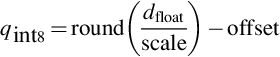
In the formula, round() is the rounding function, scale is a FP32 floating-point number, q_uint8 is an unsigned 8-bit integer, and offset is an INT32 number. The data range is [scale*offset, scale*(255 + offset)]. If the value range of the data to be quantized is [d_min, d_max], the scale and the offset are calculated as follows:
The weight value and the data are both quantized by using the solution of the aforementioned formula, and d_min and d_max are the minimum value and the maximum value of the to-be-quantized parameter.
For the quantization of the weight value, because the weight value is determined when the inference acceleration is performed, the weight value does not need to be calibrated. In the algorithm, d_max and d_min can directly use the maximum value and minimum value of the weight value. According to the algorithm verification result, for the convolutional layer, each convolution kernel adopts one independent quantization coefficient, and the precision of inference is high after quantization. Therefore, the quantization of the convolutional layer weight value is performed according to the number of convolution kernels, and the calculated scaling ratio and the number of the quantization offset are the same as the number of the convolution kernels. For the fully connected layer, the weight value quantization usually uses one set of scaling ratios and quantization offset.
Data quantization is to collect statistics on input data of each layer to be quantized, and each layer calculates an optimal set of scaling ratios and quantization offset. Because data is an intermediate result of inference calculation, the range of data is related to input, and a group of reference (the dataset used for inference) input needs to be used as an example to obtain the input data of each layer to determine d_max and d_min for quantization. In practice, the test dataset is often sampled to obtain a small batch of the dataset for quantization. Because the range of the data is related to the input, to make the determined [d_min, d_max] better robust when the network has different input data, a solution of determining the [d_min, d_max] based on the statistical distribution is proposed. The difference between the statistical distribution of the quantized data and the one of the original high-precision data is calculated and the optimal [d_min, d_max] is calculated by minimizing the difference, which leads to the optimal [d_min, d_max], and the offset and scale can be computed thereafter based on the calculation result.
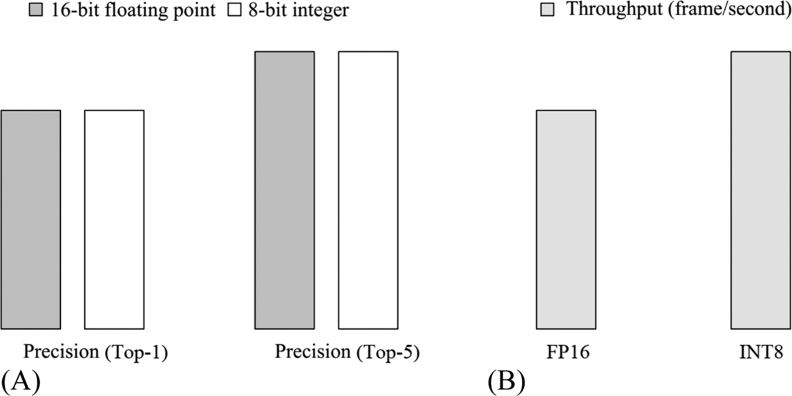
In this case, for the residual network of 152 layers, as shown in Fig. 6.18, a throughput increase of about 50% may be obtained by using a precision cost of less than 0.5%. Quantification plays a significant and practical role in typical industrial application scenarios.
6.3: Object detection
6.3.1: Dataset: COCO
Although ImageNet provides tags for object detection and localization tasks, the most commonly used dataset in this area is the COCO dataset sponsored by Microsoft Corporation, which consists of a large number of daily scene images containing everyday objects. It provides richer data for object detection, semantic segmentation, and text annotation with pixel-level annotations, which facilitates training and evaluation of object detection and segmentation algorithms. Every year, this dataset is used for a competition, which covers typical machine vision applications such as object detection, semantic segmentation, key point estimation, and image captioning (the contextual relationship between objects). It is one of the most influential academic competitions since the ILSVRC.
Compared to ImageNet, COCO consists of images, which contain objects with the scene background, i.e., noniconic images. As shown in Fig. 6.19, such an image can better reflect the visual semantics and is more in line with the requirements of image understanding. In contrast, most images in the ImageNet dataset are iconic images, and these are more suitable for image classification, as it is less affected by the semantics.
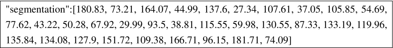
The COCO object detection task consists of 80 object categories and 20 semantic categories. The 2014 version of the COCO dataset includes 82,783 training images, 40,504 validation images, and 40,775 testing images. The basic format of the dataset is shown in the following table, where the instance segmentation annotates the exact coordinates of each control point on the boundary with a precision of two decimal places. For example, we randomly select an imagee from COCO dataset which can be described using the text “Two black food boxes with a variety of cooked foods.” To illustrate the polygon segmentation annotation, Fig. 6.20 shows a sequence of boundary points, each in (x, y) pair, which belongs to the “Broccoli” object in the image. Note that a single object that is occluded may require multiple polygons to represent it. There are also data labeled by traditional bounding boxes (corresponding to the “bbox” field in the image annotation json file). The meaning of the four numbers is the top left horizontal coordinate, the top left vertical coordinate, the width, and the height (the unit is pixel). More descriptions and data downloading instructions can be found in the COCO dataset official website.f
As mentioned in the first section of this chapter, the evaluation criteria for object detection is more complicated than image classification. The COCO dataset provides more refined criteria, which not only facilitates the data visualization and evaluation but can also help analyze the underlying reasons for typical model errors and identify any shortcomings of the algorithms.
For example, the evaluation criteria provided by COCO includes the mean Average Precision (mAP) based on different Intersection over Union (IoU) thresholds. In terms of the mAP, the evaluation metrics used by COCO are as follows:
- • AP: The IoU starts from 0.5, with a step size of 0.05, to 0.95. The mean of the average precision of all 80 categories is computed at each of the 10 IoU thresholds. This is the major evaluation metric for the COCO object detection challenge.
- • AP0.5: When the IoU is 0.5, the mean average precision of all categories, which is the same as the PASCAL VOC evaluation metrics.
- • AP0.75: When the IoU is 0.75, the mean of the average precision of all categories, which is stricter than the previous one.
Compared with ImageNet, which focuses on single object localization, the objects to be detected in COCO are smaller and more complex. The “small object” with an area of 32*32 square pixels or less accounts for 41% of the objects. The “medium object” with an area between 32*32 and 96*96 square pixels accounts for 34%, and the rest 24% is “large object” with an area over 96*96 square pixels. To better evaluate the algorithms, COCO also uses the mean average precision based on the size of the object as follows:
- • APS: Mean average precision on the “small object”: the area is within 32*32 square pixels.
- • APM: Mean average precision on the “medium object”: the area is between 32*32 and 96*96 square pixels.
- • APL: Mean average precision on the “large object”: the area is above 96*96 square pixels.
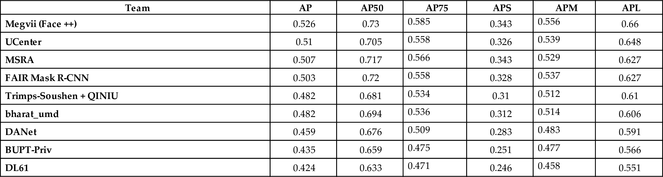
Besides, the recall rate in the field of object detection describes the number of objects detected out of all the objects in the image. For example, if there are five birds in the image, and the model only detects one, then the recall rate is 20%. For the average precision, COCO also considers the number of repeated calls of the algorithm (repeated detection of each image or 1 time, 10 times, and 100 times) and the different scales of the object, and uses the average recall rate as an important evaluation criterion. These standards established by COCO have gradually been recognized by the academic community and became a universal evaluation standard. It can also be seen in Table 6.2 that the small objects (APS) have lower mean average precision than the large object (APL). In general, smaller objects are more challenging to detect. In addition, when the IoU is 0.5, the mean average precision is higher. It is largely because the mAPs of all 80 categories obtained at the three IoU thresholds of [0.85, 0.90, 0.95] are significantly lower. Especially for small objects, it is generally difficult to achieve a 90% IoU.
Ever since ResNet achieved milestone results on ImageNet in 2015, the subsequent image recognition competitions are no longer as attractive for major companies and universities as it was before. The reason is that after the performance of the algorithm gradually approaches or even surpasses the performance of human, it is difficult for researchers to make subversive improvements in the algorithm. Therefore, the organizing committee chose to end the competition, and researchers moved to the MS-COCO object detection task. As shown in Table 6.3, the best algorithm utilizing the MS-COCO has a mean average precision of only about 53%. Therefore, there are significant rooms for improving state-of-the-art algorithms in object detection. Furthermore, complex object detection algorithms are widely used in the industry, to enable applications such as autonomous driving, smart security, smart city, and many other areas that need to parse and analyze complex scenes in images for abstraction and analysis. Also, the demand for real-time object detection is very high. Considering autonomous driving as an example, limited by the transmission bandwidth of the internet and environmental conditions, hundreds of image frames and sensor data need to be processed and analyzed per second on the device side. Only when decisions can be made within milliseconds in such systems, the safety of the passengers can be guaranteed.
Table 6.3
| Team | AP | AP50 | AP75 | APS | APM | APL |
|---|---|---|---|---|---|---|
| Megvii (Face ++) | 0.526 | 0.73 | 0.585 | 0.343 | 0.556 | 0.66 |
| UCenter | 0.51 | 0.705 | 0.558 | 0.326 | 0.539 | 0.648 |
| MSRA | 0.507 | 0.717 | 0.566 | 0.343 | 0.529 | 0.627 |
| FAIR Mask R-CNN | 0.503 | 0.72 | 0.558 | 0.328 | 0.537 | 0.627 |
| Trimps-Soushen + QINIU | 0.482 | 0.681 | 0.534 | 0.31 | 0.512 | 0.61 |
| bharat_umd | 0.482 | 0.694 | 0.536 | 0.312 | 0.514 | 0.606 |
| DANet | 0.459 | 0.676 | 0.509 | 0.283 | 0.483 | 0.591 |
| BUPT-Priv | 0.435 | 0.659 | 0.475 | 0.251 | 0.477 | 0.566 |
| DL61 | 0.424 | 0.633 | 0.471 | 0.246 | 0.458 | 0.551 |
6.3.2: Algorithm: YoloV3
In the previous section, the residual block was explained and the focus was mostly given on explaining the depth and precision of neural networks. In this section, the Yolo model is demonstrated, and the attention is given more on the speed of network inference. From the first version of Yolo (named from You Only Look Once, meaning “you just have to look at it once,” only one convolution block is required) to the third version, the primary objective is to make the object detection as fast as possible. The low precision for small object detection, which is the shortcomings of the previous versions, has been well overcome in YoloV3, and it has become the most cost-effective algorithm so far.
As shown in Table 6.4, under similar hardware configurations, YoloV3 is 100 times faster than the Region-based Convolution Neuron Network [13] (RCNN) and 4 times faster than the Fast Region Convolutional Neural Network [14] (FastRCNN). Furthermore, YoloV3 is 3 times faster than the similar algorithm Single Shot Multibox Detection [15] (SSD) and even more accurate. YoloV3 provides a cost-effective solution for commercial applications with its ability to perform real-time video analysis based on lower-cost hardware, making it one of the most commonly used models for video processing in industrial practices.
Table 6.4
| Method | mAP | Inference time (ms) |
|---|---|---|
| SSD321 | 28.0 | 61 |
| DSSD321 | 28.0 | 85 |
| R-FCN | 29.9 | 85 |
| SSD513 | 31.2 | 125 |
| DSSD513 | 33.2 | 156 |
| FPN FRCN | 36.2 | 172 |
| RetinaNet-50-500 | 32.5 | 73 |
| RetinaNet-101-500 | 34.4 | 90 |
| RetinaNet101-800 | 37.8 | 198 |
| YOLOv3-320 | 28.2 | 22 |
| YOLOv3-416 | 31.0 | 29 |
| YOLOv3-608 | 33.0 | 51 |
The performance data in the figure is based on the NVIDIA M40 or Titan X graphics card (recreated).
Based on the article “Focal Loss for Dense Object Detection” [16], the commonly used algorithms for object detection can be roughly classified into three categories. The first is the traditional object detection algorithm. Based on the sliding window theory, windows of different sizes and aspect ratios are used to slide across the whole image with certain step size, and then the areas corresponding to these windows are classified. The Histograms of Oriented Gradients [17] (HOG) published in 2005 and the Deformable Part Model [18] (DPM) proposed later are representatives of traditional object detection algorithms. Based on the carefully designed feature extraction method, these algorithms obtain excellent results in certain fields such as human pose detection. After the emergence of deep learning, the traditional image processing algorithms gradually fade out due to the lack of competitiveness in accuracy.
Deep-learning based object detection models can be divided into two groups. The first group is two-stage models. The core idea is similar to the traditional object detection algorithms. The first step is to select multiple high-quality region proposals from the image that probably corresponds to real objects. The next step is to select a pretrained convolutional neural network (such as VGG or ResNet as described above), “cut the waist” at a layer before the fully connected layer and take out the “front half” of the network (layers starting from the input image and to the selected layer) as the feature extractor. The features extracted with the feature extractor for each region proposal are then resized into fixed size required by the successive layers. Based on these features, the successive layers predict the categories and bounding boxes, which are further compared with the ground-truth categories and bounding boxes to train the classifier and the regression model. For example, if the object to detect is “cat,” the network is trained to predict the category of the region proposal to be “cat” and regress the bounding box to fit the ground-truth boundary box of “cat.” The two-stage models have developed for years from “Selective Search for Object Recognition” [19] and recently evolved to the R-CNN series, while the first stage mostly involves a selective search to extract the region proposals which contain important information of the target objects, and the second stage is to perform classification and regression based on the features extracted upon the region proposals. However, because such algorithms require extracting the features for each region individually, overlapping regions can cause a large amount of redundant computation. A major improvement of Fast R-CNN over R-CNN is that, based on the shift invariance of the convolution operator, the forward inference of the convolutional neural network is only needed to perform once on the image to map the positions of objects from the original image to the convolutional feature map. In addition, Faster R-CNN further improves the efficiency of selective search by using the neural network to predict the candidate object boundary. However, there is still a gap in real-time video analysis.
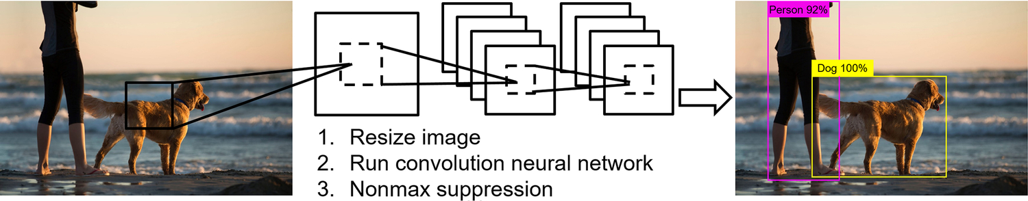
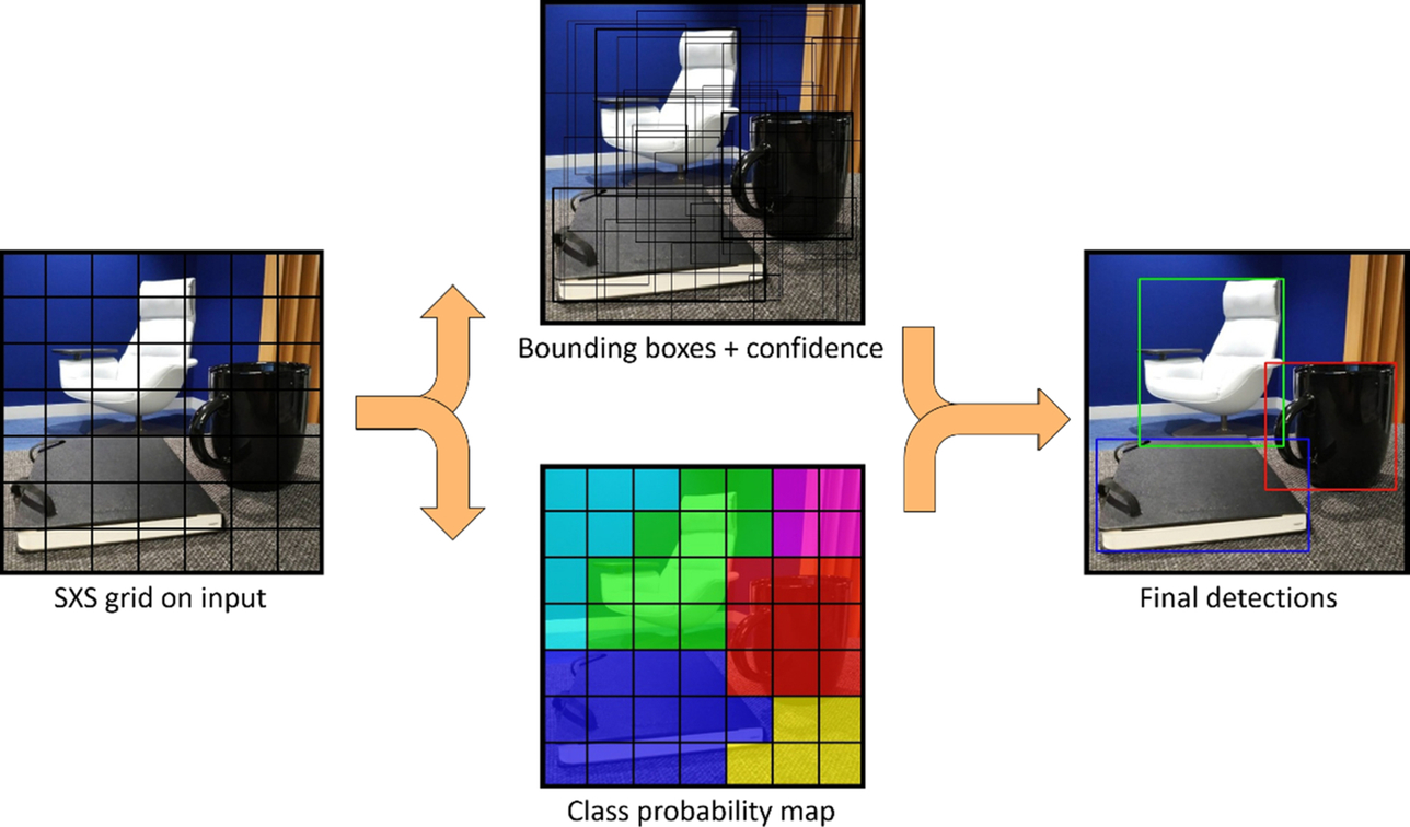
The second group is one-stage algorithms that use only one network to predict the categories and locations of objects. Algorithms such as SSD and Yolo belong to one-stage methods. The general pipeline of the algorithm is shown in Fig. 6.21. First, the image is resized, and then features are extracted by the convolutional neural network. Then the results are filtered by nonmaximum suppression, and the bounding boxes, as well as the categories, can be obtained at one shot. In short, it treats the object detection as a regression problem and predicts the labels directly from the image. As can be seen in Fig. 6.21, the two-stage methods are relatively complex and slower, but it has high precision. The one-stage techniques are simple and straightforward with a faster speed, but the mean average precision is relatively lower. In practice, developers can choose the optimal algorithm and hardware architectures based on their business needs and scenarios.
In the first Yolo model, which was published in 2015, the author borrowed the network structures from the popular GoogleNet at the time and attached two fully connected layers to the 24-layer convolutional network, using 1*1 convolution to control the feature dimensions. At the last layer, the author used a linear activation function to predict a 7*7*30 vector matrix. The meaning of 7*7 here is simple and clear. You can refer to the leftmost image in Fig. 6.22. The image is divided into 7*7 small squares (feature maps) and each square region corresponds to its detection result, which is represented as a feature vector of 1*30. For each square region, the authors attempt to predict two target bounding boxes. Defining a bounding box needs four floating-point values: the center point coordinates (x, y) of the bounding box and the width and height (w, h) of the bounding box. The prediction of the bounding box also produces a confidence value, i.e., the probability of the bounding box representing an object. So the number of predicted values of each bounding box is 4 + 1 = 5. Two bounding boxes require 5*2 = 10 floating-point values. The remaining 20 floating-point numbers are used for prediction of class labels—20 categories in total since YOLO initially used PASCAL VOC for training. Thus, since each of the 7*7 squares generates 20 + 10 = 30 floating-point numbers, a 7*7*30 matrix is generated by the network at the end.
The reader can change the number of regions for dividing the image, the number of bounding boxes for each region, and the number of categories to be predicted, based on the characteristics of the data and its applications. Assuming that the image is divided into S*S small regions, each region corresponds to B bounding boxes, and C classes need to be predicted, then the only work is to define the regression target of the neural network a matrix of S*S*(B*5 + C) and retrain or fine tune the network parameters. It should be noted here that a small square in the image corresponds to two bounding boxes, but the two bounding boxes share the same probability value of a particular category. This results in less satisfactory detection results of Yolo for close objects and small objects.
To improve the accuracy under the premise of high performance and to solve the problem of missing the detection of small and close objects, two newer versions of the Yolo network was developed. In a later version, the authors bind the predicted category probabilities to each bounding box. In YoloV2, the authors use a 19-layer Darknet network structure to extract features, and use a couple of techniques such as high-resolution classifier, batch normalization, convolutional with anchor boxes, dimension clusters, and multiscale training, to improve the efficiency and accuracy of the model. In YoloV3, the authors borrow the idea of the residual network, which is mentioned in the previous section, and set a shortcut structure on the 53-layer Darknet network to extract image features. Based on the concept of Feature Pyramid Networks, the authors further modify the network structure and adjust the input size to 416*416, and use feature maps in three scales (the image is divided in three ways 13*13, 26*26, 52*52, respectively). Fine-grained features and the residual network bring a higher level of abstraction, which improves the detection accuracy of YoloV3 for small objects and hence boosting its popularity in industrial practice.
6.3.3: Customized operator practice
Similar to the previous image classification practice, after obtaining the weight file and configuration file of the YoloV3 model from the official websiteg of the author Joseph, the first step is to convert the existing YoloV3 model into the .om format, which is supported by the Ascend AI processor. In this tutorial, the focus is on the process of developing customized operators, so the original implementation of the convolution operators is intentionally removed from the framework. Readers can get all the source code for this use case from the official website of Huawei’s Ascend AI processor.h In the fifth chapter of this book, we explained how to implement a Reduction operator in the TBE domain-specific language. In this section, we will use the typical two-dimensional convolution operator as an example to illustrate the end-to-end process of customizing a convolution operator and integrating it into networks.
When the reader attempts to convert models from other frameworks into DaVinci offline models through the offline model generation commands mentioned in the image classification section, if there are undefined operators in the model, “operator unsupported” errors can be found in the log files for offline model generation. At this point, you may choose to implement a customized operator. It is notable that when the user redefines the operators that are already supported in the framework and the names are exactly the same (e.g., the two-dimensional convolution operator Conv2D has been defined in the framework, and the reader also implements a new Conv2D operator), the convertor will choose the user’s new implementation.
To customize the TBE operator, you need to implement the logic for both Compute and Schedule. Compute describes the computational logic of the algorithm itself, and Schedule describes the scheduling mechanism of the algorithm on the hardware side, including the way to implement the computational logic such as network splitting and data stream. The split of Compute and Schedule resolves the problem of strong coupling of computational logic and hardware implementation, making computing independent from scheduling. Compute can be reused as a standard algorithm on different hardware platforms. After Compute is implemented, the hardware-related mechanism is designed based on the data stream of the computation. Furthermore, to make the customized operators visible to the framework, the customized operators need to be registered with plugins.
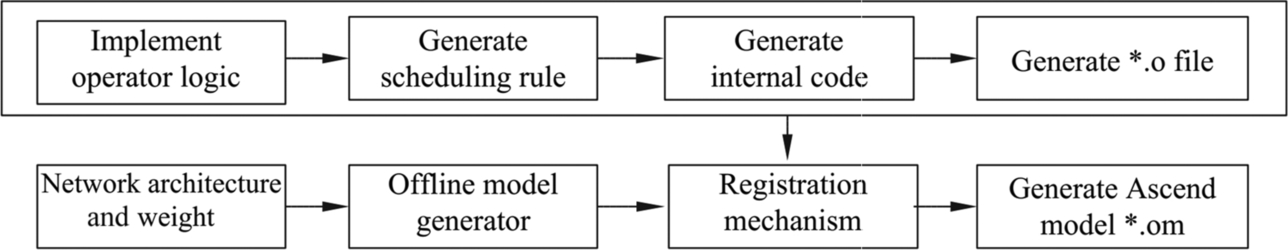
As shown in Fig. 6.23, the implementation of the operator logic (including Img2Col matrix expansion, MAD matrix multiplication, etc.) is decoupled from hardware. That is to say, the task scheduling of the operators on the processor side, such as data stream and memory management, is automatically generated by independent scheduling modules. After integration with computational logic and task scheduling, TBE generates cce codes. Then the cce codes are compiled into executable files by the offline model generator through the plug-in mechanism. The .om model file supported by the Ascend AI processor is generated based on the original network weights and configuration files. When individual operators of the current model are not supported, users can develop customized operators in this way and enable the inference of customized models from end to end. Next, let’s look at the implementation of the plugin module, operator logic module, and scheduling generation module step by step.
6.3.3.1: Development of plugin
The development of the plugin is similar to what has been described in the programming section. After the offline model generator is launched, the plugin mechanism is called first to notify the framework that the current operator is a user-defined TBE operator and then registers the operator into the framework. So before defining the operator, you need to complete the development of the plugin, so that the executable file which supports the new operator can be generated successfully in the subsequent model conversion.
Specifically, the primary function of the plugin is to establish the correspondence between the name of the DaVinci operator and that of the Caffe operator in the offline model generator, so that the offline model generator can find the dll (dynamic link library) file corresponding to the needed operator during conversion. The customized operator with the same name of the Caffe operator is registered and the executable file for the current operator is generated in a specified path. After conversion, the customized operator is packaged into the DaVinci model to form an .om file. Inference can be done by the offline model directly during the offline model execution phase. It should be noted here that the dll file compiled by the plugin is on the host side and it belongs to the preprocessing stage of model conversion.
The registration of the plugin requires the following items:
- • The name of the operator: conv_layer, defined by the user;
- • Type of framework: CAFFE (i.e., the framework on which the model trained);
- • Operator name in the original framework (here we use Caffe): “Convolution,” note that the operator name should be exactly the same as the name in the prototxt file for Caffe model;
- • The method used to derive the shape and type of the output: For example, for InferShapeAndType_conv, its implementation can be referred to as the derivation of tensor shape in the Caffe framework. For the activation function, the shape of the input and the output tensor is the same. Users may implement the functions in other ways as needed;
- • Compilation method for the target files of the operator: for example, BuildTeBin_conv;
- • Method for executing the operator parsing: TVM;
- • Data format: DOMI_TENSOR_NC1HWC0;
- • Arrangement of weights: DOMI_TENSOR_FRACTAL_Z;
This book has mentioned many times that when a matrix larger than 16*16 is used for computation, it is recommended to store the matrix in a specific data format in advance, and to read the data in specific tiles during the computation. The way of data arrangement specifies the way of data reading, which is represented by DOMI_TENSOR_FRACTAL_Z. In the next section about the implementation of operators, the details of the data arrangement and computations based on the tiling strategy will be further explained.
To sum up, the way to define a typical operator plugin is presented in Code 6.6:
6.3.3.2: Implementation of the operator
Different from the implementation of the CPU, the implementation of a convolution operator on the Ascend AI processor is more complicated. In order to make full use of the computing power of the Cube Unit, it is necessary to change the input data format in advance, such as arrangement, expansion, and dicing. This section will elaborate on how to implement the convolution operator on the AI Core with a given configuration.
Matrix operation based on Cube Unit
The most basic operations that can be performed by the Cube Unit on the Ascend AI processor are matrix multiplications with input size Mcube × Kcube and Kcube × Ncube. The Cube Unit supports three data types: FP16, INT8, and UINT8. The value of Mcube, Kcube, and Ncube differs by data type, as illustrated in Table 6.5.
Table 6.5
| Data type | Mcube | Kcube | Ncube |
|---|---|---|---|
| INT8 | 16 | 32 | 16 |
| UINT8 | 16 | 32 | 16 |
| FP16 | 16 | 16 | 16 |
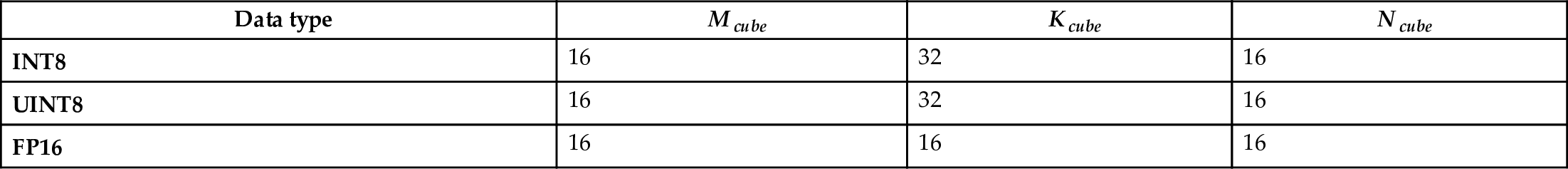
In order to support matrix multiplication operations of any input size, e.g., matrix A of size M × K and matrix B of size K × N, the input matrices need to be partitioned in advance. To be specific, you need to pad M to multiples of Mcube, K to multiples of Kcube, and N to multiples of Ncube, so that the matrix A can be partitioned into a block matrix of size ![]() (each block is Mcube × Kcube), and matrix B can be partitioned into a block matrix of size
(each block is Mcube × Kcube), and matrix B can be partitioned into a block matrix of size ![]() (each block is Kcube × Ncube). Then matrix multiplication is performed on each pair of blocks. For example, each multiplication is between two matrices with the size of Mcube × Kcube and Kcube × Ncube, and each addition is between two matrices with the size of Mcube × Ncube.
(each block is Kcube × Ncube). Then matrix multiplication is performed on each pair of blocks. For example, each multiplication is between two matrices with the size of Mcube × Kcube and Kcube × Ncube, and each addition is between two matrices with the size of Mcube × Ncube.
Definition of convolution operator parameters and data arrangement
A convolution operator takes an input feature map and a convolution kernel as input, and generates an output feature map.
As mentioned in Chapter 4, in deep learning framework, the feature map data of the convolutional operator is generally arranged in the format of NHWC or NCHW, where:
- • N: The number of sample images in a batch of input data.
- • H: The height of the feature map.
- • W: The width of the feature map.
- • C: The number of channels of the feature map.
On the CPU, the feature map data in the memory is generally arranged in the NHWC format. In order to facilitate the presentation, the shape of the input feature map is written as NHinWinCin, and the output feature map shape is written as NHoutWoutCout.
The shape of the convolution kernel is written as CoutCinHkWk, where:
- • Cout: The number of convolution kernels, which is equivalent to the number of channels in the output feature map.
- • Cin: The number of weight matrices in each convolution kernel, which is equivalent to the number of channels in the input feature map.
- • Hk: The height of the weight matrix in the convolution kernel.
- • Wk: The width of the weight matrix in the convolution kernel.
In addition, the convolution operator generally has the following parameters:
- • Ph: Padding size (one side) along the height of the feature map.
- • Pw: Padding size (one side) along the width of the feature map.
- • Sh: The stride size of the convolution along the height of the feature map.
- • Sw: The stride of the convolution along the width of the feature map.
Accordingly, the height and width of the output feature map are obtained by the following formula:
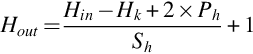
Example of the Convolutional operator
In order to facilitate the explanation, we assume that the data type is FP16 and all the parameters mentioned above are represented with the following specific values:
- • N = 10
- • Cin = 32
- • Cout = 64
- • Hin = Win = Hout = Wout = 28
- • Hk = Wk = 3
- • Ph = Pw = 1
- • Sh = Sw = 1
In this case:
- • The shape of input feature map [N, Hin, Win, Cin], i.e., [10, 28, 28, 32].
- • The shape of kernel weights [Cout, CinHk, Wk], i.e., [64, 32, 3, 3].
- • The shape of the output feature map [N, Hout, Wout, Cout], i.e., [10, 28, 28, 64].
Format conversion of the input feature map
The format conversion of the input data involves the following steps:
- Step 1. The input data in the NHWC format is converted into the 5D format of NC1HWC0 defined under the DaVinci architecture.
- Step 2. The 5D format of NC1HWC0 is expanded into the 2D format of the input feature map matrix by the Img2Col method.
- Step 3. Based on the “small Z big Z” rule, the memory arrangement of the input feature map matrix is converted.
On the Ascend AI processor, the data is saved in the 5D format of NC1HWC0, where C0 is related to the DaVinci architecture and is equal to Kcube, and C1 is the quotient of Cin divided by C0, which can be expressed as ![]() , as shown in Fig. 6.24. The specific conversion process is as follows:
, as shown in Fig. 6.24. The specific conversion process is as follows:
- Step 1. The Cin of the input feature map data [N, Hin, Win, Cin] is split based on Kcube to obtain
 , i.e., [10, 28, 28, 32] is split into [10, 28, 28, 2, 16]. If Cin is not a multiple of Kcube, you need to pad zeros to reach the multiple of Kcube and then split.
 - Step 2. Dimensional permutation of gives
 , i.e., [10, 28, 28, 2, 16] is further converted to [10, 2, 28, 28, 16].

The illustration of the entire conversion process is shown in Fig. 6.25. This process takes place in two scenarios:
- • The first layer of RGB image data needs to be converted.
- • The output feature map data for each layer needs to be rearranged.
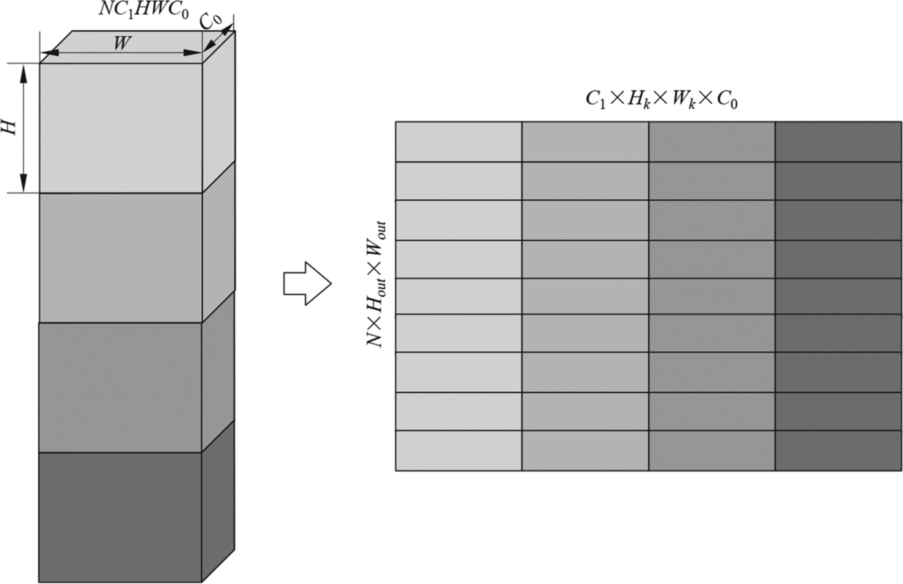
After converting the input feature map into the 5D NC1HWC0 format, according to the Img2Col algorithm, the data needs to be converted into a 2D format, namely the input feature map matrix. Based on the Img2Col algorithm described above, the shape of the final input feature map matrix is [N, HoutWout, HkWkCin], where HoutWout the height is and HkWkCin is the width. As shown in Fig. 6.25, since the Cin dimension is split by the Ascend AI processor, the shape of the final input feature matrix is ![]() , i.e.,[10, 28 ⁎ 28, 2 ⁎ 3 ⁎ 3 ⁎ 16], i.e., [10,784, 288].
, i.e.,[10, 28 ⁎ 28, 2 ⁎ 3 ⁎ 3 ⁎ 16], i.e., [10,784, 288].
After Img2Col conversion, the input feature map matrix needs to be further converted into the “small Z big Z” layout format, so further splitting and conversion of the axis are needed. Finally, the shape of the input feature map block format is ![]() , where HoutWout is padded to the multiple of Mcube and then split. Considering the example mentioned above, the output shape should be [10, 49, 18, 16, 16]. It can be seen that [16, 16] are the height and width of the small matrix, respectively, so it is called the “small Z” arrangement. [49, 18] are the height and width of the block format of the input feature map matrix, respectively. It is called the “big Z” arrangement.
, where HoutWout is padded to the multiple of Mcube and then split. Considering the example mentioned above, the output shape should be [10, 49, 18, 16, 16]. It can be seen that [16, 16] are the height and width of the small matrix, respectively, so it is called the “small Z” arrangement. [49, 18] are the height and width of the block format of the input feature map matrix, respectively. It is called the “big Z” arrangement.
The two steps above are done by dedicated hardware in the AI Core. The implementation of the hardware is relatively complicated due to the need to complete all the conversions simultaneously. Fig. 6.26 shows the process of further conversion using the example for calculating the parameters for the convolution kernel given in the previous section, which includes the following steps:
- Step 1. Since the step sizes Sh and Sw are both 1, in order to obtain a small matrix at coordinate (0, 0) in the input feature map matrix (a total of 49*18 small matrices), it is necessary to sequentially read 16*16 = 256 number of data in the input feature map, whose shape is [Mcube, Kcube] and can be directly expanded into a small matrix. It is equivalent to unfolding the pixel points at (0, 0) for the Kcube = 16 convolution kernels.
- Step 2. Continue to read 256 number of data, and a small matrix at coordinate (0,1) can be obtained, which is equivalent to expanding the pixel points at coordinate (0, 1) for the Kcube = 16 convolution kernels. During the process of data reading, based on the different stride sizes, some data may be read multiple times and the hardware can use these data during the conversion process.
- Step 3. Continue to get a small matrix at coordinate (0,2), which is equivalent to expanding the pixels at coordinate (0,2) for the Kcube = 16 convolution kernels.
- Step 4. After the first three steps, Wk = 3 small matrices have been obtained along the width of the input feature graph matrix, and then the input feature map need to be expanded along with the other Hk = 3 dimensions. Repeat step 1–3 to expand pixel points of (1,0), (1,1), (1,2), (2,0), (2,1), (2,2) for the Kcube = 16 convolution kernels.
- Step 5. After Steps 1–4, HkWk = 9 small matrices have been obtained along the width of the input feature map matrix. Next is to do a further expansion for
 dimensions by repeating Steps 1–4.
 - Step 6. After Steps 1–5, all the
 small matrices have been obtained along the width of the input feature map. Then further expansion is done along with the height of the input feature map for
  dimensions by repeating Step 1–5.
 - Step 7. After Step 1–6, the last to do is do a further expansion for N dimensions (the batch size of the input feature map), and Step 1–6 is then repeated.
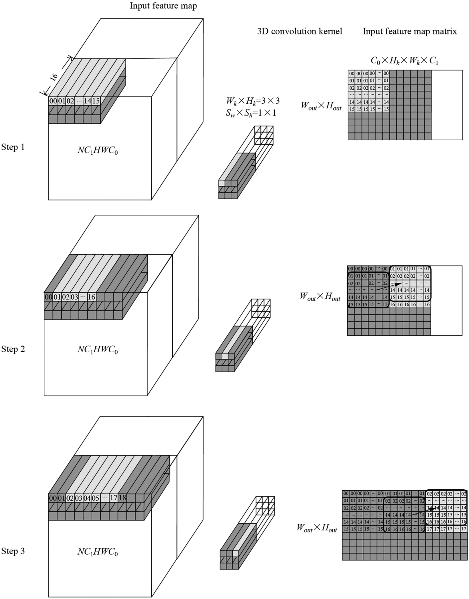
After all the steps above, we finally get 10*49*18 = 490*18 small matrices and convert the input feature map into the input feature matrix with the format of “big Z small Z.” The final shape of the data is [10, 49, 18, 16, 16].
Format conversion of the weight data
The format conversion of weight data includes the following steps:
- Step 1. The weight data is also converted into the 5D format of NC1HWC0, and finally the data of the format
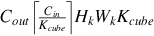 is obtained.
 - Step 2. The 5D format of NC1HWC0 is expanded into a 2D format of the weight matrix.
- Step 3. The memory arrangement of the weight matrix is further converted based on “big Z small Z.”
The steps above are completed offline by the offline model generator during the model conversion process, and the data can be directly loaded during inference on the Ascend AI processor.
The shape of the weight data is [Cout, Cin, Hk, Hw], i.e., [64, 32, 3, 3], and after converted to 5D format, the shape becomes ![]() , i.e., [64, 2, 3, 3, 16].
, i.e., [64, 2, 3, 3, 16].
Since the data conversion is completed offline and the speed is not a concern, the 5D to 2D and the “big Z small N” conversion can be conducted separately. As shown in Fig. 6.27, the weight data needs to be converted into a weight matrix, which is relatively simple to implement. The convolution kernel data of each Kcube(or C0) channels are expanded into a column vector, and these column vectors are horizontally concatenated, forming a part of the weight matrix with the shape of [HkHwKcube, Cout], i.e., [144, 64]. After that, the operation is repeated along the height direction of the weight matrix for ![]() dimensions, and the final weight matrix
dimensions, and the final weight matrix![]() (i.e., [288, 64]) can be obtained.
(i.e., [288, 64]) can be obtained.
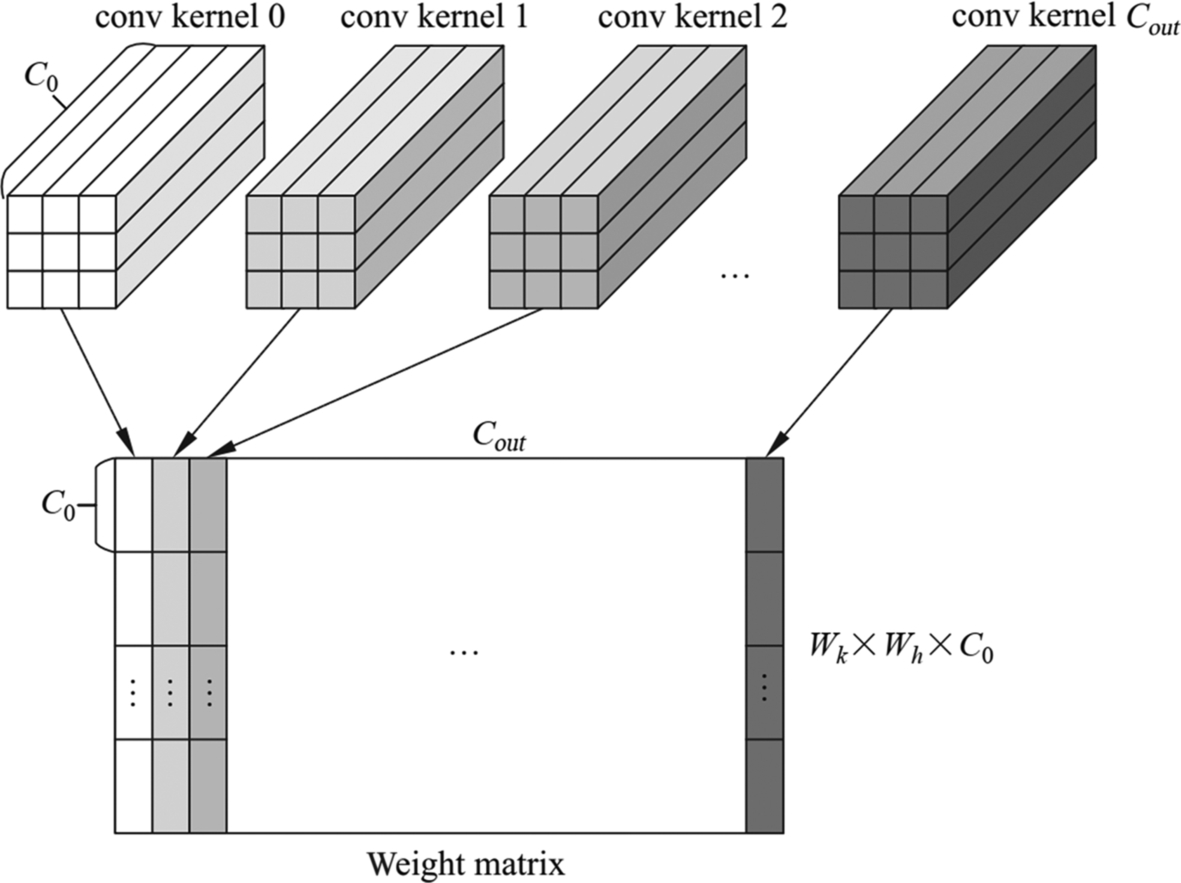
After Img2Col conversion, the weight matrix needs to be further converted into a “big Z small N” layout format. Therefore, further splitting and conversion of the axis are needed. Finally, the shape of the weight matrix block format is ![]() (i.e., [18, 4, 16, 16] for the previous example), where Cout needs to be padded to the multiple of Ncube. It can be seen that [16, 16] are the width and height of the small matrix, arranged based on the column-major, so it is called “small N” arrangement; [18, 4] are the height and width of the weight matrix block format, arranged based on the row-major, so it is called “big Z” arrangement.
(i.e., [18, 4, 16, 16] for the previous example), where Cout needs to be padded to the multiple of Ncube. It can be seen that [16, 16] are the width and height of the small matrix, arranged based on the column-major, so it is called “small N” arrangement; [18, 4] are the height and width of the weight matrix block format, arranged based on the row-major, so it is called “big Z” arrangement.
Based on the steps above, 18*4 small matrices are finally obtained, and the weight matrix is constructed based on the format of “big Z small N,” and the final shape of the converted data is [18, 4, 16, 16].
Format conversion of the output feature map
The shape of the input feature map matrix is ![]() , i.e., [10, 49, 18, 16, 16]; the weight matrix shape is
, i.e., [10, 49, 18, 16, 16]; the weight matrix shape is ![]() , i.e., [18, 4, 16, 16].
, i.e., [18, 4, 16, 16].
The multiplication of the two matrices is done in two steps:
- Step (1) The small matrices are multiplied. In specific, two small matrices of size Mcube × Kcube and Kcube × Ncube are multiplied to obtain a small matrix of size Mcube × Ncube. For the previous example, two small matrices of size 16 × 16 are multiplied to obtain a small matrix of size 16 × 16.
- Step (2) The block matrix is multiplied, and the dimension N is placed in the width of the input feature map matrix, that is, block matrices of size
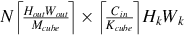 and
and  are multiplied to obtain a block matrix of size
 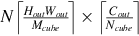 . Specifically, two-block matrices of size 490 × 18 and 18 × 4 are multiplied to obtain a block matrix of size 490 × 4.
AI Core’s Cube Unit directly supports small matrix multiplication, which can be computed with one instruction. The resulting small matrix is stored in the format of row-major, i.e., “small Z” arrangement, and the shape is [Mcube, Ncube], i.e., [16, 16].
For the multiplication of block matrices, it is very similar to regular matrix multiplication. However, the AI Core uses the operation order as shown in Fig. 6.28. That is, the input feature map matrix traverses the small matrices in column-major, the weight matrix traverses the small matrices in row-major, and the output feature map stores the small matrices in column-major. Among the three dimensions of matrix multiplication, the loop numbers are loop(M) = 490, loop(K) = 18, loop(N) = 4. The strategy is to compute the loops from the outside to the inside, i.e., op(K) → loop(N) → loop(M). So the small matrices of the final output feature map are stored in column-major, i.e., “big N” arrangement, and the data format is ![]() , i.e., [4, 490]. The corresponding pseudo code is shown in Code 6.7. There are several points to note about such a loop strategy:
, i.e., [4, 490]. The corresponding pseudo code is shown in Code 6.7. There are several points to note about such a loop strategy:
- • Having the loop with the most iterations, i.e., loop(M), as the innermost loop helps to improve the loop efficiency.
- • Put loop(K) as the outermost loop so that the partial accumulation results obtained in each loop and the partial results stored in the buffer, obtained by multiple loops can be accumulated into the final result.
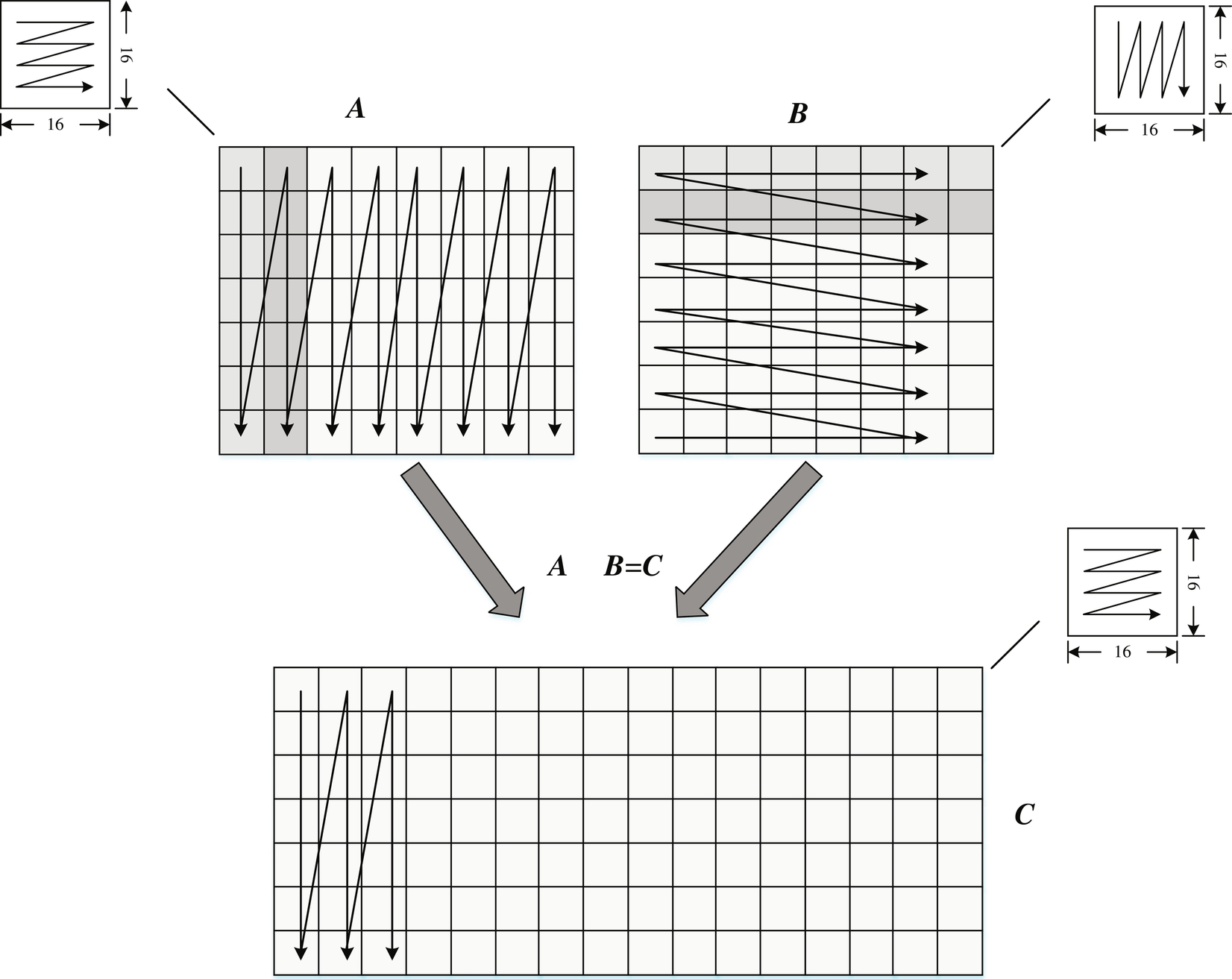
After all the steps above, 490*4 small matrices are obtained, and the output feature map matrix is constructed in the format of “big N small Z,” and the final shape is [4, 490, 16, 16].
The shape of the output feature map matrix is ![]() , i.e., [4, 490, 16, 16]. In the process of data transfer, a specific reading strategy can be used to remove the redundancy caused by zero paddings, and the obtained data shape is
, i.e., [4, 490, 16, 16]. In the process of data transfer, a specific reading strategy can be used to remove the redundancy caused by zero paddings, and the obtained data shape is ![]() , i.e., [4, 10,28,28,16]; then through the dimension conversion, we can get the 5D layout format of the output feature map data
, i.e., [4, 10,28,28,16]; then through the dimension conversion, we can get the 5D layout format of the output feature map data ![]() , i.e., [10, 4, 28,28,16]. For the data type of FP16, Ncube = Kcube = 16, so the resulting output feature map shape is
, i.e., [10, 4, 28,28,16]. For the data type of FP16, Ncube = Kcube = 16, so the resulting output feature map shape is ![]() , i.e., [10, 4, 28, 28, 16], which is the 5D format of NC1HWC0 specified for the AI processor.
, i.e., [10, 4, 28, 28, 16], which is the 5D format of NC1HWC0 specified for the AI processor.
Furthermore, if the batch size dimension N of the feature map is placed in the outermost loop of Code 6.7, the shape of the output feature map matrix is ![]() . By removing the redundancies, it can be rearranged as
. By removing the redundancies, it can be rearranged as ![]() (i.e., [10, 4, 28, 28, 16]) without performing dimension conversion. Both loop methods introduced above are used in practice and can be selected based on specific needs.
(i.e., [10, 4, 28, 28, 16]) without performing dimension conversion. Both loop methods introduced above are used in practice and can be selected based on specific needs.
At this point, the whole process of using the Cube Unit for the convolutional operation on AI Core is completed. This operation can be implemented with the TVM primitives. The Ascend AI software stack has encapsulated the implementation of computing and scheduling into an interface te.lang. Cce.conv. Readers can refer to the TVM implementation provided in DDK if interested.
6.3.3.3: Performance analysis
Looking back at the beginning of this section, when the offline model generator generates the offline model yolov3.om, the error log shows there are unsupported operators.i At this point, since the reader has completed the development of the convolutional operator computing logic and plugins, the next step is just to copy the completed plugin codes to the installation folder of the ddk package, find the TOPDIR parameter in the corresponding makefile and modify it to the directory where the plugin is located, and compile the plugin.
Once the plugin has been successfully compiled, you can generate the .om model using the same commands at the beginning of this section. Here, the .om model is executed in the same way as the image recognition case. You can refer to the commands shown in Code 6.8.
The object detection results given by YoloV3 are shown in Fig. 6.29. Each image can contain multiple detection bounding boxes, and the category with the highest confidence is used as the detection result. Since the primary strength of YoloV3 is speed, this section focuses on the efficiency of YoloV3 and how the customized convolution operators implemented on the AI CPU and AI Core will affect the throughput of the YoloV3 model.
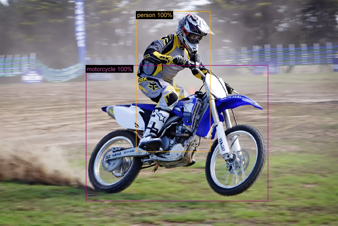
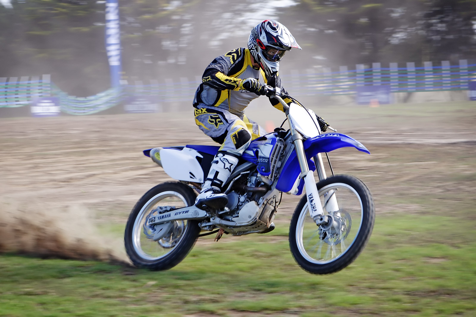
For the convolutional layers, the total number of operations required is assessed in a simple way. Assume that the number of convolution kernels in the current layer is Cout and the convolution kernel size is Wk ⁎ Hk, the input feature map channel number is Cin, the size of the output data in the horizontal direction is Wout, and the size of the output data in the vertical direction is Hout. The required number of operations for the current convolutional layer is (in GFLOPS, 1 TFLOPS = 10ˆ3 GFLOPS):
Based on this, the number of operations of the first 10 layers of YoloV3 can be analyzed as shown in Table 6.6. Following this method, it is not difficult to find that the total number of operations required for the 105 layers of the entire YoloV3 is 65.86 GFLOPS.
Table 6.6
| #Layers | Operator | #Conv kernels | Conv kernel | Input shape (H*W*C) | Output shape (H*W*C) | #Operations (GFLOPs) |
|---|---|---|---|---|---|---|
| 0 | conv | 32 | 3 * 3/1 | 416 * 416 * 3 | 416 * 416 * 32 | 0.299 |
| 1 | conv | 64 | 3 * 3/2 | 416 * 416 * 32 | 208 * 208 * 64 | 1.595 |
| 2 | conv | 32 | 1 * 1/1 | 208 * 208 * 64 | 208 * 208 * 32 | 0.177 |
| 3 | conv | 64 | 3 * 3/1 | 208 * 208 * 32 | 208 * 208 * 64 | 1.595 |
| 4 | res | 1 | 208 * 208 * 64 | 208 * 208 * 64 | ||
| 5 | conv | 128 | 3 * 3/2 | 208 * 208 * 64 | 104 * 104 * 128 | 1.595 |
| 6 | conv | 64 | 1 * 1/1 | 104 * 104 * 128 | 104 * 104 * 64 | 0.177 |
| 7 | conv | 128 | 3 * 3/1 | 104 * 104 * 64 | 104 * 104 * 128 | 1.595 |
| 8 | res | 5 | 104 * 104 * 128 | 104 * 104 * 128 | ||
| 9 | conv | 64 | 1 * 1/1 | 104 * 104 * 128 | 104 * 104 * 64 | 0.177 |
| 10 | conv | 128 | 3 * 3/1 | 104 * 104 * 64 | 104 * 104 * 128 | 1.595 |
| … | ||||||
| 104 | conv | 256 | 3 * 3/1 | 52 * 52 * 128 | 52 * 52 * 256 | 1.595 |
| 105 | conv | 255 | 1 * 1/1 | 52 * 52 * 256 | 52 * 52 * 255 | 0.353 |
| blank cell | 65.862 |
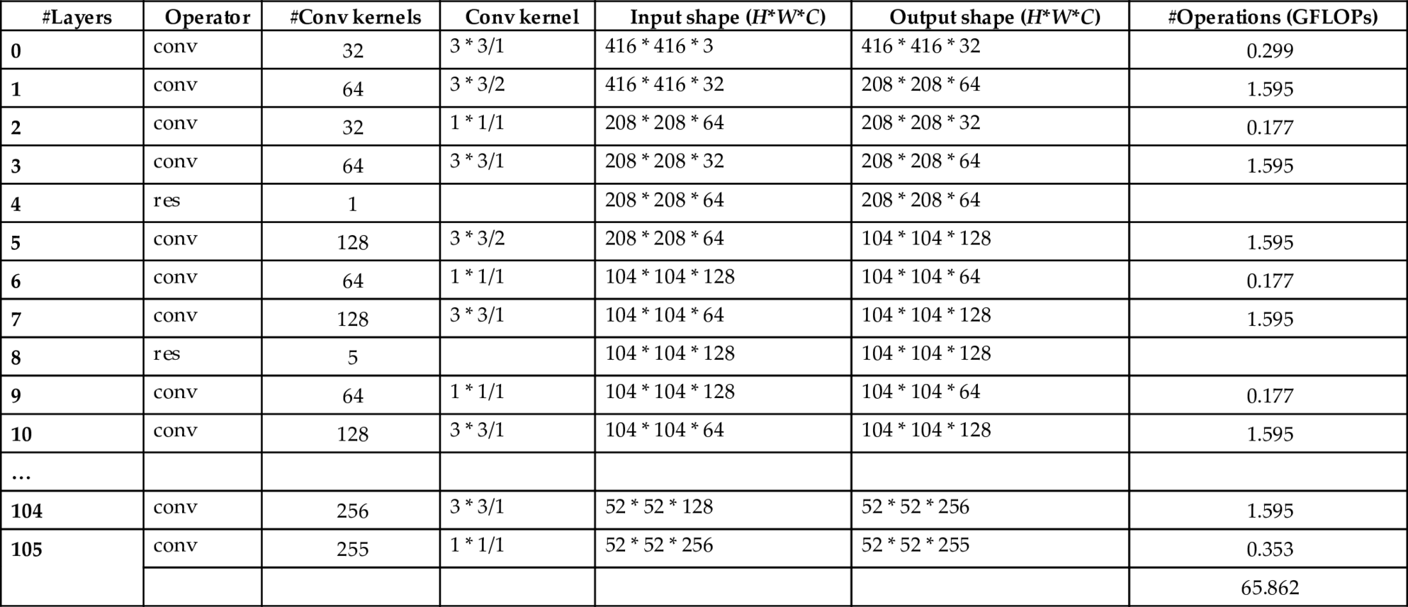
The core of the DaVinci architecture is the Cube Unit, which can perform the multiply-accumulate computation of two 16*16 FP16 matrices per instruction, that is, perform 4096 multiply-accumulate operations. On a typical CPU, only one multiply-accumulate operation can be performed under each instruction. Assume that within the same period of time, the number of instructions that the CPU can execute is 4 times more than that of the AI Core. However, the execution efficiency of the CPU is a 1000 times worse than the AI Core. Of course, the end-to-end throughput of the computing hardware does not entirely depend on its computing power. It is also affected by multiple factors, such as memory transfer and task scheduling. Assuming the computation time when the Cube Unit is fully loaded is Tc, and the task scheduling and data transfer time required on the AI CPU and the AI Core are similar and are represented by Td, the estimated time on the AI Core is:
The time required on the AI CPU is:
Furthermore, if assuming the time Tc of the full-load computation in the Cube Unit is to be p times larger than Td, with the ratio of the execution time on the AI Core and the AI CPU as the vertical axis R, curves can be drawn as shown in Fig. 6.30. In Fig. 6.30A, p ranges from 0.01 to 10 with a step size of 0.01; in Fig. 6.30B, p ranges from 0.0001 to 0.01 with a step size of 0.0001. It is easy to see that as the value of p increases, the advantage of the AI Core becomes increasingly significant, but the growth rate gradually slows down and eventually converges to the theoretical limit. When p is small, as shown in (Fig. 6.30B), which is also a more common situation in practice, the ratio R of the computational efficiency on the AI Core to the AI CPU can be approximated by a linear function.

For the implementation of the TBE operator, the Compute and Schedule are implemented separately, and it means the computation logic and the scheduling logic are separated. With the change of one single line of code, the convolutional operator can be implemented either on the AI CPU or AI Core.
The implementation of AI Core is:
sch = auto_schedule(tensor_list[-1])
The implementation on the AI CPU is:
sch = cpu_schedule(tensor_list[-1])
Taking the YoloV3, which has 65.86 GFLOPS as an example, the convolution operator is implemented on the AI CPU and the AI Core, respectively, and the ideal throughput ratio produced is as shown in the Fig. 6.31 (here Batch Size = 1). Of course, the specific implementation of the customized operator (especially the way of data segmentation) will also affect the resource utilization of the Cube Unit in the AI Core, thus affecting the computational efficiency. However, in general, when performing a large number of matrix multiplication operations, the operators will be arranged on the AI Core as much as possible; when the amount of computation is small, or the parallelization is difficult, the operators will be arranged on the AI CPU for better computational efficiency. In this case, since the Ascend 310 single processor has the computing power of 16 TOPS for INT8, if the model is quantized to INT8, the theoretical throughput limit is:

In practice, it is also necessary to concern about the time of task scheduling and data transfer, and the utilization rate of the Cube Unit often cannot reach 100%. So, the measured running time will be negatively affected, which can only reach half of the theoretical limit.
Another factor that has a tremendous impact on throughput is the number of input images per batch (i.e., Batch Size, BS). Similar to other dedicated processors, for the Ascend AI processor, a larger Batch Size can often lead to better performance and can increase the gap between the performance for FP16 and INT8. Fig. 6.32 shows the throughput of the two commonly used image recognition networks VGG19 and ResNet50 with different Batch Sizes on the ImageNet dataset. It is easy to observe that for INT8, increasing the Batch Size from 1 to 8 doubles the performance of ResNet and triples the throughput for VGG19. Therefore, the user can choose the appropriate number of images per batch in practice to achieve an optimal balance between throughput and response time.

6.3.3.4: Performance improvement tips
In summary, given the characteristics of the Ascend 310 processor, to improve the performance of the algorithm, it is necessary to maximize the utilization rate of the Cube and reduce the ratio of data transfer and Vector computation. In general, consider the following tips:
- (1) Network structure selection
It is recommended to use mainstream network structures. For example, the image recognition networks can be selected from the built-in networks such as ResNet and MobileNet, as the performance of these networks has been optimized. For object detection, similarly, it is recommended to use mainstream detection networks, such as FasterRCNN, SSD, etc., as their performance has been optimized.
It is not recommended to use obsolete network structures, such as VGG, AlexNet, etc., because the model sizes of these networks are enormous, the bandwidth pressure is high, and the accuracy of these models is lower than that of the ResNet.
As shown in Fig. 6.33, the M, K, N in the matrix multiplication should be taken as multiples of 16. The algorithm should consider increasing the number of channels as appropriate, rather than reducing the number of channels by grouping.
Fig. 6.33 Illustration of matrix multiplication (left matrix size M*K, right matrix size K*N, output matrix size M*N).
Increasing data reuse rate: more times of a parameter is used, lower bandwidth utilization rate will be. Therefore, the algorithm should consider increasing the number of times for reusing the convolution kernels, such as increasing the feature map sizes or avoiding large stride sizes. - (2) Convolution (Conv) operator
In FP16 mode, the number of input and output channels of the convolution operator is recommended to be a multiple of 16.
In INT8 mode, the number of input and output channels of the convolution operator is recommended to be a multiple of 32.
In INT8 mode, between multiple convolution operators, it is recommended to insert as few pooling operators as possible. - (3) Fully connected (FC) operator
When there is a fully connected operator in the network, try to perform inference with more images in a batch. - (4) Concatenation (Concat) operator
In FP16 mode, the channel number of the input tensor of the concatenation operator is recommended to be a multiple of 16.
In INT8 mode, the channel number of the input tensor of the concatenation operator is recommended to be a multiple of 32. - (5) Operator fusion
It is recommended to use a combination of Conv + BatchNorm + Scale + ReLU, whose performance has been optimized. - (6) Normalized operator
It is recommended to use the BatchNorm operator and use pretrained normalization parameters.
It is not recommended to use operators that need to calculate normalized parameters online, such as LRN [20]. - (7) Techniques for optimizing the performance of typical operators
The performance of Conv +(BatchNorm + Scale) + ReLU is better than the performance of Conv +(BatchNorm + Scale) + tanh. As shown in Fig. 6.34, complex activation functions should be avoided.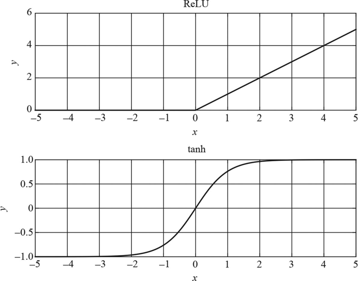
Fig. 6.34 Illustration of the typical activation functions. The computational complexity of the ReLU operator (upper) is significantly lower.
When the concatenation operator is used on the channel (C) dimension, the performance is better when the number of channels of the input tensor is a multiple of 16.
The fully connected operator performs better when the batch size is a multiple of 16.
Continuous convolution operators perform better; if more Vector operators (such as Pooling) are inserted between convolutional layers, the performance will go down. This is especially obvious for the INT8 model.
In earlier convolutional networks such as AlexNet and GoogleNet, LRN was used as the normalization operator. The computation of this operator is very complicated. During the evolution of the algorithms, it was gradually replaced with other implementation methods such as BatchNorm. In the current mainstream network structures such as ResNet and Inception, LRN is not used anymore. If you want to maximize the performance on the Ascend AI processor, it is recommended to replace the LRN operator with BatchNorm in the network.