
Chapter 2: Industry background
Abstract
This chapter focuses on the AI industry background. Firstly, the current status of popular neural network processors is introduced, including CPU, GPU, TPU, FPGA, and Huawei Ascend AI processor. Then, it is explained how CPU and GPU accelerate neural network. In the next part, the popular deep learning software frameworks are introduced, including Caffe, Tensorflow, Pytorch, and Huawei’s MindSpore. At the end of the chapter, the idea of intermediate representation (IR) and deep learning compilation framework is illustrated, which helps migrate algorithms between different frameworks. As an example, tensor virtual machine (TVM) is explained in detail.
Keywords
Huawei ascend AI processor; CPU; GPU; TPU; FPGA; Caffe; Tensorflow; Pytorch; MindSpore; TVM
With the rapid development of deep learning, Nvidia continues to focus on its GPU processors and has launched the Volta [1] and Turing [2] architectures to continuously meet deep learning’s requirements for huge computing power. Microsoft also uses FPGAs in its data centers instead of CPUs to complete computationally intensive tasks [3]. Google specifically designed the TPU processor for the deep neural network, marking the rise of the domain-specific architecture (DSA) [4]. In this environment, Huawei has also launched its self-developed Ascend AI processor, which aims to provide higher computing power and lower energy consumption for deep learning research, development, and deployment [5].
Over time, deep learning open-source software frameworks have become increasingly mature and provide efficient and convenient development platforms [6]. These frameworks allow researchers to focus on algorithm research while enjoying hardware acceleration without worrying about the implementation of specific details. The collaborative development of software and hardware has become a new trend in the deep learning field.
2.1: Current status of the neural network processors
2.1.1: CPU
In the process of computer development, central processing unit (CPU) plays an irreplaceable role. Early computer performance steadily improved year by year with Moore’s Law [7] and met the needs of the market. A large part of this improvement was driven by the progress of underlying hardware technologies to accelerate the upper-layer application software. In recent years, physical bottlenecks such as heat dissipation and power consumption have made the growth of CPU performance slower than what is predicted by Moore’s Law, indicating traditional CPU architectures are reaching their limits. As a result, the performance of serial programs operating under traditional CPU architectures cannot be significantly improved. This has led the industry to continuously search for new architectures and software frameworks for the post-Moore’s law era.
As a result, multicore processors have emerged to meet the requirements of hardware speed requested by software. Intel’s i7 series processors, based on the x86 instruction set, use four independent kernels to build an instruction parallel processor core, which improves the processor running speed to a certain extent. However, the number of kernels cannot be increased infinitely, and most traditional CPU programs are written in serial programming mode due to costs or difficulty of expressing them in a parallel form. As a result, a large number of programs cannot be accelerated.
In the trend of AI industry development, deep learning has become a hot spot. Its demand for computing power and memory bandwidth is becoming more and more intense. Traditional CPUs are insufficiently confronted with the huge demand for computing power required by deep learning. Since CPUs are facing great challenges in terms of both software and hardware, the industry must try to find new alternatives and develop new processors that can implement large-scale parallel computing suitable for deep learning. A revolution in the computer industry has come.
2.1.2: GPU
The GeForce GTX 280 graphics card launched by Nvidia in the early stage uses the graphics processing unit (GPU) composed of multicore streaming multiprocessors (SM). Each stream processor supports a multithread processing mode called single instruction multiple threading (SIMT). This large-scale hardware parallel solution brings breakthroughs in high throughput operations, especially floating-point computing performance. Compared with multicore CPU, GPU design does not start from the instruction control logic or expand the cache. Therefore, complex instructions and data access do not increase the delay. On the other hand, GPUs use a relatively simple storage model and data execution process, which relies on discovering the intrinsic data parallelism to improve throughput. This leads to greatly improved the performance of many modern data-intensive programs compared to CPUs. Due to its unique advantages, the GPU has gradually been adopted into the domain of supercomputing applications and has deeply changed the fields of automatic driving, biomolecular simulation, manufacturing, intelligent video analysis, real-time translation, and artificial intelligence through deep learning [8].
The architecture of GPUs is different from that of CPUs. CPUs focus on logic control in instruction execution while GPUs have a prominent advantage in the parallel computing of large-scale intensive data. To optimize a program, it is often necessary to use the respective capabilities of both CPUs and GPUs to perform collaborative processing. In this model, the CPU can flexibly process complex logical operations and hybrid computing of multiple data types while the GPU is needed to schedule rapid large-scale parallel computing. Generally, CPUs perform the serial part of the program well, whereas GPUs efficiently perform parallel processing of large-scale data.
To implement the collaborative computing paradigm, new software architectures can be used to program both CPUs and GPUs in a common unified framework. Nvidia proposes a compute unified device architecture (CUDA) framework to solve complex computing problems that apply to GPUs [9]. CUDA consists of a dedicated instruction set architecture and a parallel computing engine inside the GPU. It provides direct access to the GPU hardware so that the GPU does not rely on traditional graphics application programming interface. Instead, programmers can use C-like languages to directly program the GPU, which provides a powerful capability for modern computer systems in large-scale data-parallel computing.
In addition, because the C-like language is used as core language for GPU programming, CUDA allows programmers to quickly adapt to its programming environment. This facilitates the rapid development and verification of high-performance computing solutions by developers. Because CUDA implements a complete and universal solution on GPUs, it is widely used in many common computing fields such as science, business, and industry.
With the emergence and development of deep learning technology and given their outstanding performance in matrix computing and parallel computing, GPUs have been widely used as the first dedicated acceleration processors for deep learning algorithms and have become the core computing components applied to artificial intelligence (AI). Currently, GPUs are widely used in smart terminals and data centers, and take a leading role in deep learning training. GPUs have played an indispensable role in the AI field. As a result, Nvidia has introduced improved architectures featuring Tensor Cores and launched new-generation GPU products based on the Volta and Turing architectures in order to promote the continuous development of the deep learning hardware industry.
Nvidia recently proposed a GPU TU102 processor based on the Turing architecture [2]. It supports both general-purpose computing of the GPU and dedicated neural networks. The TU102 processor uses a 12 nm manufacturing process with areas exceeding 700 mm2. A large number of tensor units are introduced inside the TU102 processor which supports multiple-precision operations such as FP32, FP16, INT32, INT8, and INT4. The processor’s technical specifications that indicate the hardware computing capability are measured by the number of floating-point operations per second (Tera FLOPs per Second, TFLOPS) or the number of integer operations per second (Tera OPs per Second, TOPS).
In the GeForce RTX 2080 Ti using the TU102 processor, FP32 performance can reach 13.4 TFLOPS [10]. It can reach 13.4 TOPS on INT32, 26.9 TFLOPS on FP16, 107.6 TFLOPS on tensor FP16, 215.2 TOPS on INT8, and an astonishing 430.3 TOPS on INT4. Total power consumption of the system is less than 300 W.
The advantage of the Turing architecture is that the original general computing framework is retained, meanwhile allowing the CUDA framework to be used in neural network modules. This is good news for developers accustomed to CUDA programming. The core idea of Turing in processing convolutional neural networks is to convert convolution to matrix operations, and then use dedicated tensor processing units to perform these operations in parallel to accelerate the overall calculation. In essence, convolution in the tensor processing unit is accelerated using highly optimized matrix multiplication, thereby improving the neural network’s performance. The Turing architecture controls the operation of the tensor unit by using a dedicated instruction.
2.1.3: TPU
With the rapid progress of AI, the demands for higher performance of processors that support deep learning algorithms are ever increasing. Despite high performance, GPUs suffer from high power consumption. The need for processors with higher performance and better efficiency has become more urgent. As early as 2006, Google has gradually developed new computing processors, known as application-specific integrated circuits (ASIC) [11], and applied them to neural networks. Recently, Google released the tensor processing unit (TPU) [4], an AI specific processor that supports the deep learning TensorFlow open-source framework.
The first-generation TPU adopts a 28 nm manufacturing technology with the power consumption of about 40 W and clock frequency of 700 MHz. To ensure that the TPU is compatible with existing hardware systems, Google designed the TPU as an independent accelerator and uses a SATA hard disk slot to insert the TPU into servers. In addition, the TPU communicates with the host through the PCIe Gen3x16 bus. The effective bandwidth can reach 12.5 GB/s.
The primary difference between GPU and TPU for floating-point calculations is that the TPU uses low precision INT8 integer number calculation. This minimizes the number of transistors required and greatly decreases power consumption while improving operation speed. In practice, this reduction of accuracy in calculations has little effect on the accuracy of deep learning applications. To further improve performance, TPUs use up to 24 MB on-chip memory and 6 MB accumulator memory to reduce access to off-chip main memory or RAM since these accesses are slow and power-hungry. In matrix multiplications and convolution operations, much of the data is reusable and can exploit data-locality. TPUs use the systolic array to optimize matrix multiplication and convolution operations, by fully exploiting data locality, reducing memory access frequencies, and reducing energy consumption. Compared with GPU’s more flexible computing models, these improvements enable the TPU to produce higher computing power with lower power consumption.
The core concept of TPUs is to keep the computing unit running by optimizing the overall architecture and data supply, thus achieving extremely high throughput. A multilevel pipeline is used in TPU operation process with multiple multiplication instructions executed to reduce delay. Unlike traditional CPUs and GPUs, the systolic array structure adopted by TPU is especially suitable for large-scale convolution operations. During the calculation process, data flows through the operation array and when the systolic array is fully loaded, maximum performance can be achieved. In addition, bit-shift operations of the systolic array can make full use of data locality in convolution calculations, which greatly reduces power consumption by not repeatedly reading data.
TPUs efficiently accelerate the most common operations in the deep neural network by using large-scale systolic arrays and large amounts of on-chip storage. Currently, TPUs are used in the Google Street View Service, AlphaGo, Cloud TPU Platform, and Google Machine Learning Supercomputers.
2.1.4: FPGA
Field-programmable gate arrays (FPGAs) are developed as hardware prototype systems in electronics [12]. While GPUs and TPUs play important roles in the AI field, FPGAs enable developers familiar with hardware description languages to quickly implement AI algorithms and achieve considerable acceleration, thanks to their highly flexible hardware programmability, the parallelism of computing resources and relatively mature toolchains. FPGAs are now widely used in artificial intelligence after years of being in a “supporting role” and have brought a new architecture choice to the industry.
The first FPGA XC2064 was launched in 1985 by Xilinx who gradually developed a series of FPGA processors dedicated to flexible programmable electronic hardware systems. Due to the need for neural network computing power, FPGAs were first applied in the field of neural networks in 1994. With the evolution of modern deep learning algorithms into more difficult and complex directions, FPGAs began to show their unique network acceleration capabilities. FPGAs consist of programmable logic hardware units that can be dynamically programmed to achieve the logical functions required. This capability enables FPGA to be highly applicable to many domains and they are widely used. Optimized properly, FPGAs feature high performance and low power consumption. The flexible nature of FPGAs gives them an unparalleled advantage compared to other hardware with fixed capabilities.
A unique and distinctive feature of FPGAs is reconfigurability. This allows reprogramming and changing the hardware functionality, allowing multiple different hardware designs to be tested in order to achieve optimal performance. In this way, optimal solutions for neural networks in a specific application scenario can be obtained. Reconfigurability is categorized into static and dynamic. The former refers to the reconfiguration and reprogramming of hardware before hardware execution in order to adapt to system functions. The latter refers to hardware reconfiguration based on specific requirements during program execution.
Reconfigurability gives FPGAs advantages in deep neural networks, but it incurs some costs. For example, reprogramming may be slow and often unacceptable for real-time programs. In addition, FPGAs have a high cost. For large-scale use, the cost is higher than dedicated ASICs. The reconfigurability of FPGAs is based on hardware description languages (HDLs) and reconfiguring often requires using HDLs (such as Verilog and VHDL) for programming. These languages are more difficult and complex than high-level software programming languages and are not easily mastered by most programmers.
In June 2019, Xilinx launched its next-generation Versal series components [13]. It is an adaptive computing acceleration platform (ACAP) and a new heterogeneous computing device. With it as the most recent example, FPGAs have evolved from a basic programmable logic gate array to dynamically configurable domain-specific hardware. The Versal adopts 7 nm technology. It integrates programmable and dynamically configurable hardware for the first time, integrating a scalar engine, AI inference engine, and FPGA hardware programming engine for embedded computing. This gives it a flexible multifunction capability. In some applications, its computing performance and power efficiency exceed that of GPUs. Versal has high computing performance and low latency. It focuses on AI inference engines and benefits from its powerful and dynamic adaptability in automatic driving, data center, and 5G network communication.
2.1.5: Ascend AI processor
In this fierce competition within the AI field, Huawei has also begun to build a new architecture for deep learning. In 2018, Huawei launched the Ascend AI processor (as shown in Fig. 2.1) based on its own DaVinci architecture and began Huawei’s AI journey.
Stemming from fundamental research in natural language processing, computer vision and automatic driving, the Ascend AI processor is dedicated to building a full-stack and all-scenario solution for both cloud and edge computing. Full-stack refers to technical aspects, including IP, processor, driver, compiler, and application algorithms. All-scenario refers to wide applicability, including public cloud, private cloud, edge computing, IoT industry terminals, and consumer devices.
To cooperate applications, an efficient operator library and highly automated neural network operator development tool were built called the Compute Architecture for Neural Network (CANN). Based on this full-stack and all-scenarios technology, Huawei uses these processors as the driving force to push AI development beyond limits in the future.
In October 2018, Ascend AI processor series products named 910 and 310 were launched. The computing density of the Ascend 910 processor is very large due to using advanced 7 nm manufacturing processes. The maximum power consumption is 350 W while FP16 computing power can reach 256 TFLOPS. The computing density of a single processor is higher than that of a Tesla V100 GPU from the same era. INT8 computing capability can reach 512 TOPS and 128 channel full HD video decoding (H.264/H.265) is supported. The Ascend 910 processor is mainly applied to the cloud and also provides powerful computing power for deep learning training algorithm. The Ascend 310 processor launched in the same period is a powerful artificial intelligence System on Chip (SoC) for mobile computing scenarios. The processor uses a 12-nm manufacturing process. Maximum power consumption is only 8 W with FP16 performance up to 8 TFLOPS, INT8 integer performance of 16 TOPS, and integrated 16-channel HD video decoder. The Ascend 310 processor is intended primarily for edge computing products and mobile devices.
In terms of design, the Ascend AI processor is intended to break the constraints of AI processors in power consumption, computing performance, and efficiency. The Ascend AI processor adopts Huawei’s in-house hardware architecture and is tailored to the computing features of deep neural networks. Based on the high-performance 3D Cube computing unit, the Ascend AI processor greatly improves computing power per watt. Each matrix computing unit performs 4096 multiplications and additions in one instruction. In addition, the processor also supports a multidimensional computing mode including scalar, vector, and tensor, which exceeds the limits of other dedicated artificial intelligence processors and increases computing flexibility. Finally, many types of hybrid precision calculation are supported for training and inference.
The versatility of the DaVinci architecture is reflected in its excellent suitability for applications with widely varying requirements. The unified architecture has best-in-class power efficiency while supporting processors from fractions to hundreds of watts. Simultaneously, the streamlined development process improves software efficiency across development, deployment, and migration for a wide range of applications. Finally, the performance is unmatched, making it the natural choice for applications from cloud to mobile to edge computing.
The DaVinci architecture instruction set adopts a highly flexible CISC instruction set. It can cope with rapidly changing new algorithms and models that are common nowadays. The efficient computing-intensive CISC architecture contains special instructions that are dedicated to neural networks and help with developing new models in AI. In addition, they help developers to quickly deploy new services, implement online upgrades, and promote industry development. The Ascend AI processor uses a scenario-based perspective, systematic design, and built-in hardware accelerators for processing. A variety of I/O interfaces enables multiple combinations of Ascend AI-based acceleration card designs, which are flexible and scalable enough to cope with cloud and edge computing and meet the challenges of energy efficiency. This allows Ascend AI-based designs to enable powerful applications across all scenarios.
2.2: Neural network processor acceleration theory
2.2.1: GPU acceleration theory
2.2.1.1: GPU computing neural networks principles
Because computations in neural networks are easily parallelized, GPUs can be used to accelerate neural networks. The major ways to accelerate neural networks with GPUs are through parallelization and vectorization. One of the most common GPU-accelerated operations in neural networks is the general matrix multiply (GEMM) since for most neural networks the core computations can be expanded into matrix operations. Convolutional neural networks are one of the most commonly used neural networks, so we take it as an example to explain how they can be accelerated with GPUs.
Convolution is the core operation of the convolutional neural network. As shown in Fig. 2.2, the convolution is illustrated with a two-dimensional input. A convolution kernel slides with a specific step size through the input image. The value of each pixel on the output image is equal to the dot product between the convolution kernel and the corresponding data block from the input image. Since GPU instructions do not directly support convolutions, to implement the operation on a GPU, the input image or feature map and convolution kernel must be preprocessed. The preprocessing is called the Img2Col. As shown in Fig. 2.2, the input image or feature map F has a size of 3 × 3 and the number of channels is 2; the convolution kernels W and G have a size of 2 × 2, and the number of convolution kernels is 2. In order to facilitate the convolution operation, the weight of each convolution kernel is first reshaped into a vector, and then the two vectors from the two channels of each convolution kernel are concatenated into one vector. The vectors from W and G are stacked as rows and finally, the corresponding 2 two-channel convolution kernels are expanded into a 2 × 8 matrix.
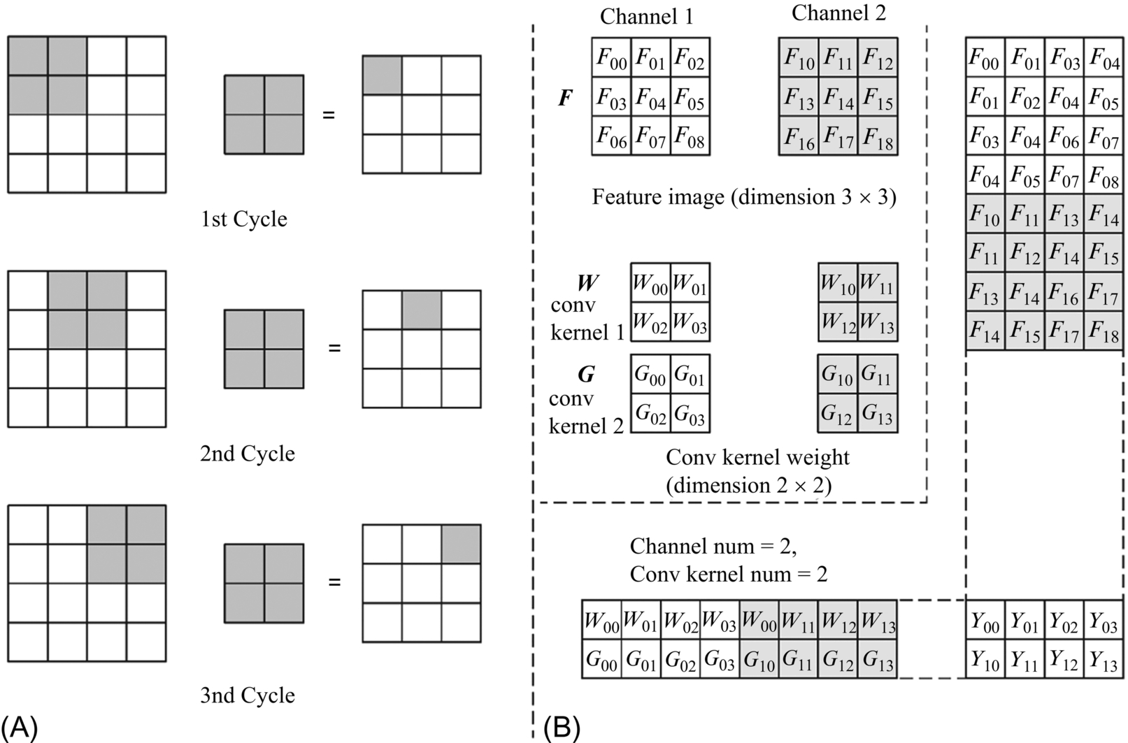
Similarly, for the input image F, the 2 × 2 block corresponding to the convolution kernel is expanded in row-major order. Consistent with the direct convolution order, the kernel slides one unit to the right and writes the block that is expanded later in the next column. Similar to the preprocessing of the convolution kernel, the two vectors of two different channels of the input image F can be concatenated into one vector and forms into the same column. Finally, a two-channel 3 × 3 input image is expanded in parallel into an 8 × 4 input feature matrix. After that, the input feature matrix is multiplied by the convolution kernel matrix, and the output obtained will be consistent with that of the traditional way of convolution.
It is worth noting that since the weights of the two channels of the same kernel have been arranged in the same row of the matrix, and the values of the two channels of the same input block are arranged in the same column, so the value of each unit of the 2 × 4 resulting matrix corresponds to the result of the accumulation of 2 channels. When the number of channels in the neural network is very large, the matrix will become so large that it might exceed the memory limit. In this way, the GPU cannot accommodate the expansion of all channels at a time. Based on the computing power of the GPU, each time an appropriate number of channels is selected and formed into an input matrix, and after some intermediate results are obtained, the outputs of multiple operations are accumulated to generate the final result.
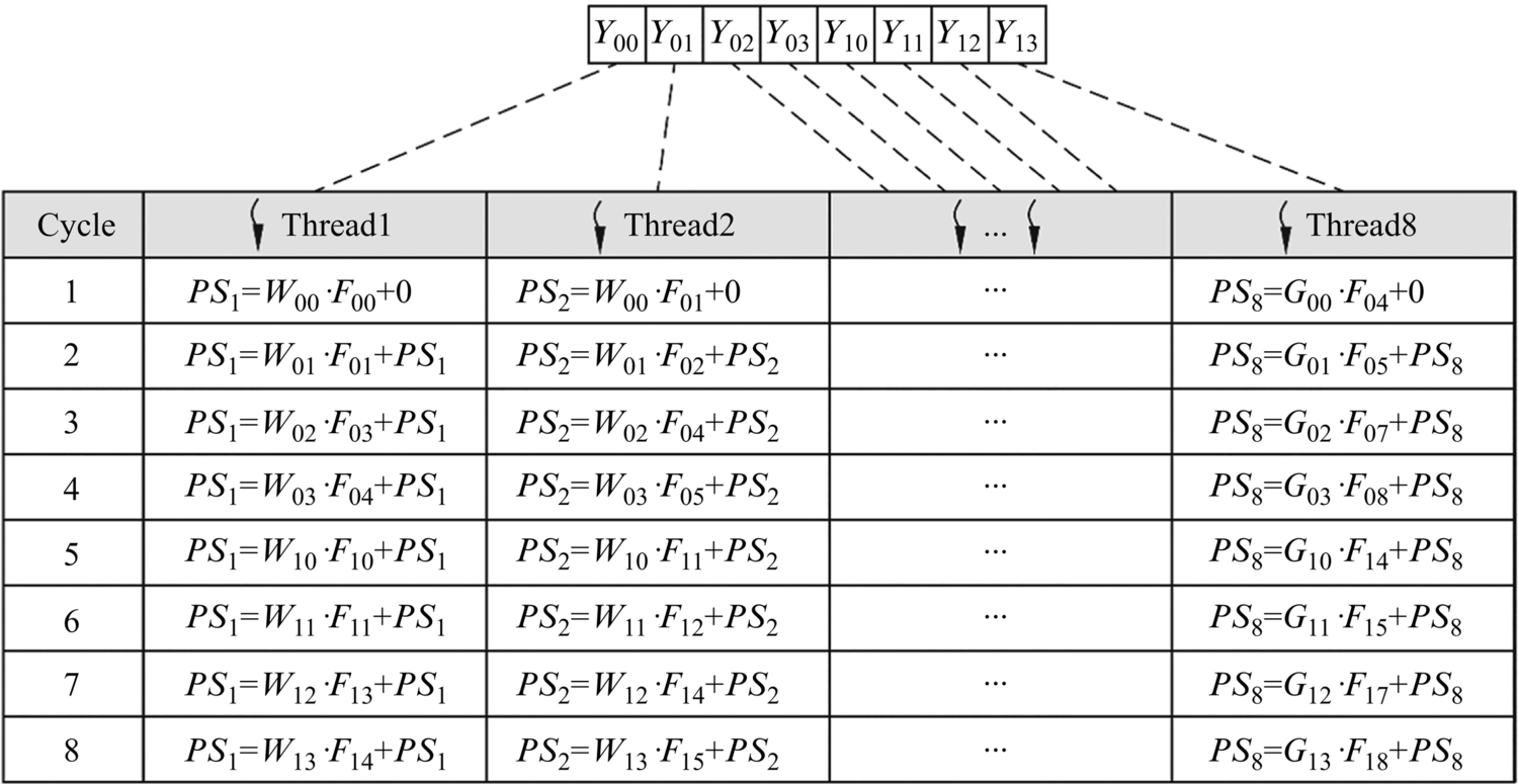
For multiplication of the expanded matrix, the GPU uses single instruction multithreading (SIMT) manner. The GPU will assign a separate thread to compute one unit of the resulting matrix, corresponding to the result of the dot product of a row of the left matrix and a column of the right matrix. For this example, the GPU can use eight threads simultaneously to compute the matrix Y in parallel, where each thread executes the same instruction stream synchronously, but on different data.
As shown in Fig. 2.3, each thread of the GPU can perform a multiply-and-accumulate operation in each cycle, with multiple threads executing independently in parallel. In the figure, PS1, PS2,⋯, PS8, respectively, represent the partial sum in each thread, which corresponds to the intermediate results in the eight elements Y00, Y01, Y02, Y03, Y10, Y11, Y12, and Y13. In each clock cycle, a thread computes the multiplication of two input numbers and accumulates it to the partial sum. Ideally, after eight clock cycles, eight parallel threads will simultaneously output eight numbers in the resulting matrix.
2.2.1.2: Modern GPU architecture
With the development of the GPU industry, Nvidia’s GPU architectures that support CUDA are also evolving from early-stage architectures like Fermi, Kepler, Maxwell, etc., which support the general floating-point computation, until the emergence of the latest architectures such as Volta and Turing that are optimized for deep learning and low-precision integer computation.
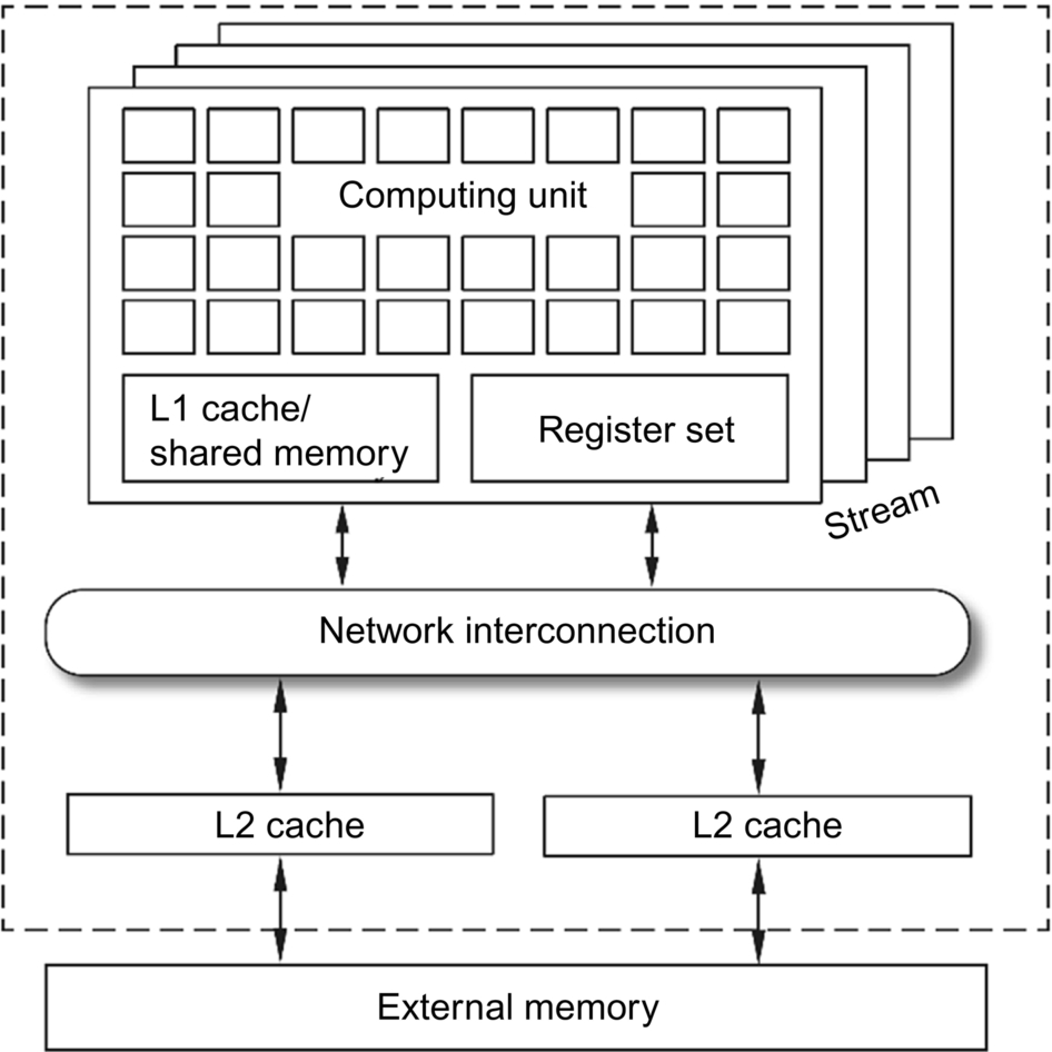
As shown in Fig. 2.4, the major functional modules of any generation of GPU architecture include stream processors, multilevel on-chip memory structures, and interconnection network structures. A complete Turing-based TU102 processor contains 72 stream processors. The storage system consists of L1 cache, shared memory, register set, L2 cache, and off-chip storage. The L2 cache size of the TU102 GPU is 6 MB.
- (1) Turing Stream Processor
In the Turing architecture [2], each stream processor contains 64 CUDA cores responsible for the computations of single-precision floating-point FP32. These CUDA cores are mainly used to support general-purpose computing programs. They can be programmed in the CUDA framework which maps to SIMT. Matrix multiplication or other types of computations can be implemented based on the methods described above.
Each stream processor in the Turing architecture also includes eight tensor cores, which is significantly different from previous generations of GPUs. The main purpose is to provide more powerful, more specialized, and more efficient computing power for deep neural network algorithms. The tensor core supports multiprecision computations such as FP16, INT8, and INT4, providing sufficient flexibility for different deep learning algorithms. With the newly defined programming interface (mainly through the use of WMMA instructions), the user can easily program the tensor core in the existing CUDA framework. The highest computational precision in the stream processor is provided by the two FP64 units, whose main target is scientific computing that have strict requirements for computational precision.
The stream processor provides space for data storage through a 256 KB register set and a 96 KB L1 cache. The large register set in the GPU is to meet the storage needs of the huge amounts of on-chip threads. Each thread running in the stream processor needs to be assigned a certain number of general-purpose registers (often used to store variables in the program). These are generally placed in the registers and directly cause an increase in the overall use of the register bank.
The GPU’s architectural design can support the use of L1 cache as shared memory. The difference between the two is that the execution of the L1 cache is completely controlled by the hardware, invisible to the programmer, and operates on the data through a cache replacement strategy similar to the CPU; and the use and allocation of the shared memory can be directly controlled by the programmer, which is extremely useful for programs with significant patterns in data parallelism.
The Turing architecture applies a new way of partitioning to improve the utilization and overall performance of the stream processor. It divides the stream processor into four identical processing zones, except that the four zones share a 96 KB L1 cache or shared memory, each of which includes a quarter of the computation and storage resources in the stream processor. Each zone is designated a separate L0 instruction cache, a warp scheduler, an instruction issue unit, and a branch jump processing unit. Compared to previous GPU architectures, the Turing architecture supports more threads, warps, and thread blocks running simultaneously. At the same time, the Turing architecture separately designed the independent FP32 and INT32 computing units, so that the pipeline can synchronize the address (INT32), and simultaneously load the data (FP32). This parallel operation increases the number of instructions transmitted per clock cycle and increases the computational speed.
The Turing architecture is designed to improve performance while balancing energy efficiency and ease of programming. It uses a specially designed multiprecision tensor core to meet the requirements of deep learning matrix operations. Compared to the older architecture, Turing’s computational throughput of floating-point numbers and integers during training and inference is greatly improved. Under the usual computational load, the energy efficiency of the Turing architecture is 50% higher than that of the earlier GPU architectures. - (2) Tensor core
Tensor core is the most important feature of Turing architecture, which can greatly improve the computational efficiency of deep neural networks. It is a new type of matrix computing unit called multiprecision tensor core. The Turing GPUs have demonstrated excellent performance in the training and inference of large-scale neural networks with the introduction of tensor cores, further stabilizing the position of GPUs in the AI industry.
There are eight tensor cores in a stream processor, supporting INT4, INT8, and FP16 multiprecision calculations. The computation precision in the tensor core is relatively low but is sufficient for most neural networks while the energy consumption and the cost of the processor are greatly reduced. Each tensor core can perform 64 times of fused multiply and add (FMA) operations with the precision of FP16 in one clock cycle, so a stream processor can achieve 512 FMA operations per clock cycle, i.e., 1024 floating-point operations. If the INT8 precision is used in the same tensor core, it will be a double performance, achieving up to 2048 integer operations per clock cycle. Using INT4, then the performance can be doubled again.
The Turing architecture supports deep neural network training and inference on the tensor core by calling the WMMA instruction. The main function of the WMMA instruction is to achieve the multiplication of the large-scale input feature matrix and the convolution kernel weight matrix in the network connection layer. The tensor core is designed to increase computational throughput and energy efficiency. When a WMMA instruction enters the tensor core, it is broken down into a number of finer-grained HMMA instructions. The HMMA instruction controls the threads in the stream processor so that each thread can complete a four-point dot-products (FEDPs) in one clock cycle.
Through careful circuit design, the tensor core ensures that each tensor core can achieve 16 FEDPs in one clock cycle, that is, each tensor core contains 16 threads. In other words, it can be guaranteed that each tensor core can complete the operation of multiplying two 4 × 4 matrices and accumulating a 4 × 4 matrix in one clock cycle. The formula (2.1) is as follows:
In formula (2.1) A, B, C, and D, each represents a matrix of 4 × 4. The input matrices A and B are FP16 precision, and the accumulation matrices C and D can be either FP16 precision or FP32 precision. As shown in Fig. 2.5, 4 × 4 × 4 = 64 multiplications and additions are needed to complete this process. The eight tensor cores in each stream processor can perform the computations above independently and in parallel.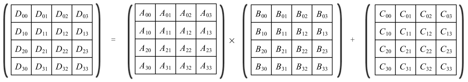
Fig. 2.5 Basic operations supported by tensor core.
When the tensor core is used to implement large matrix operations, the large matrix is first decomposed into small matrices and distributed in multiple tensor cores, respectively, and then the results are merged into a large result matrix. The Turing tensor core can be manipulated as a thread block in the interface of CUDA C ++ programming. This interface makes matrix and tensor operations in CUDA C ++ programs more efficient.
Because of the strong capabilities in accelerating neural networks, high performance numerical computing, and graphics processing of the Turning GPUs, they have had a profound impact on scientific research and engineering. Turing currently exhibits outstanding computing power in the field of deep learning. The deep network model that used to take several weeks of training time often takes only a few hours to train with Turing GPUs, which greatly promotes the iteration and evolution of deep learning algorithms. In the meantime, people are also trying to apply the massive computing power of the tensor core to other application fields beyond artificial intelligence.
2.2.2: TPU acceleration theory
2.2.2.1: Systolic array for neural networks computing
The way in which the convolution is computed in the TPU is different from that of the GPU, which mainly relies on a hardware circuit structure called “systolic array.” As shown in Fig. 2.6, the major part of the systolic array is a two-dimensional sliding array containing a number of systolic computing units. Each systolic computing unit can perform a multiply-add operation within one clock cycle. The number of rows and the number of columns in the systolic array may be equal or unequal, and the rightward or downward transfer of the data between the neighboring computing units is achieved through the horizontal or vertical data pathways.
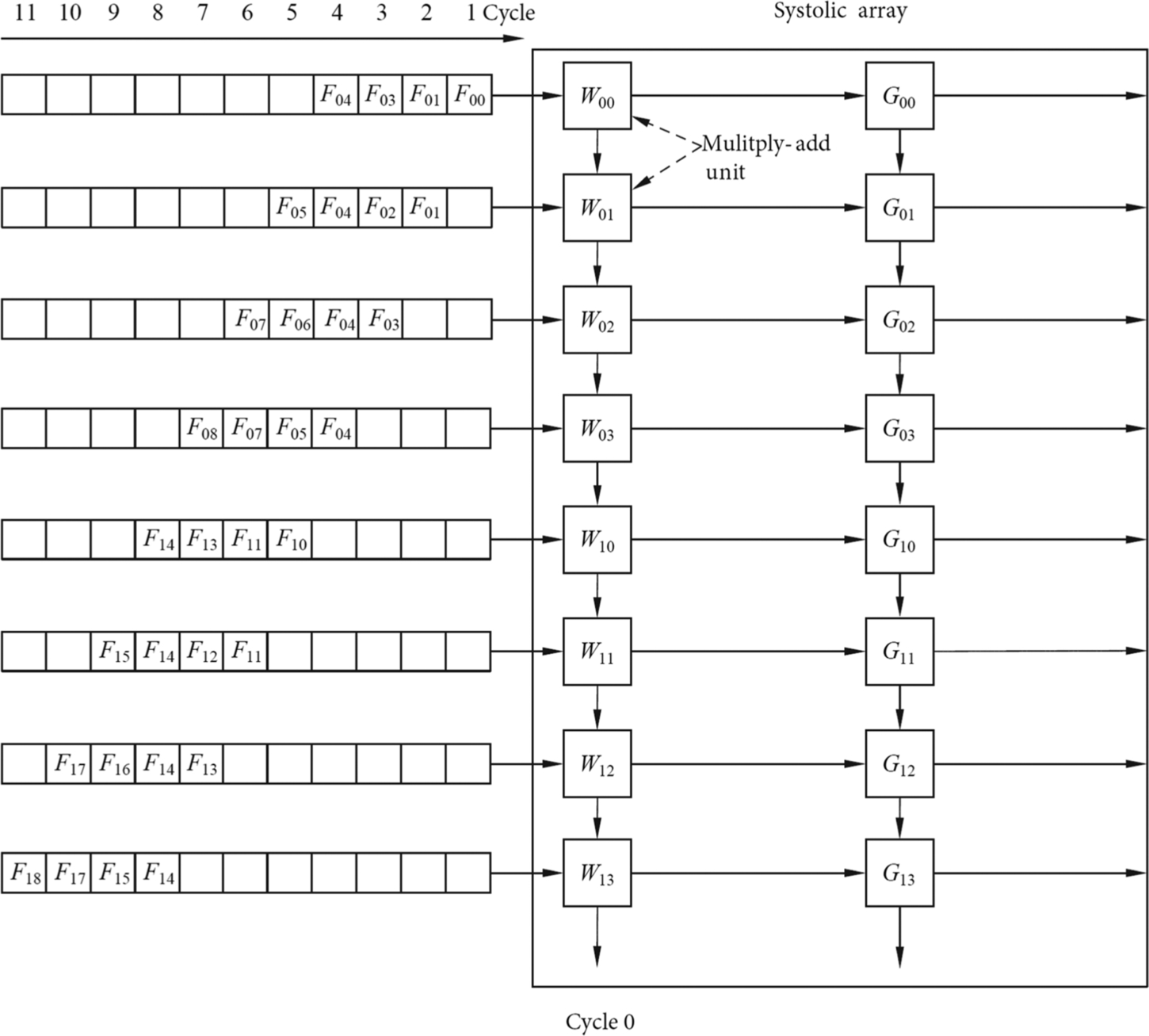
The convolutional operation in Fig. 2.2 is used as an example to explain the process of computing in a systolic array. In this example, we use fixed convolution kernel weights, and the input feature values and partial sums are transferred laterally or longitudinally through the systolic array. According to Fig. 2.6, 2 two-channel W and G convolution kernel weights are first stored in the computational unit of the systolic array, wherein the two channels of the same convolution kernel are arranged in the same column. Then, the two channels of the input features F are arranged and expanded, and each row is staggered by one clock cycle and is prepared to be sequentially fed into the systolic array.
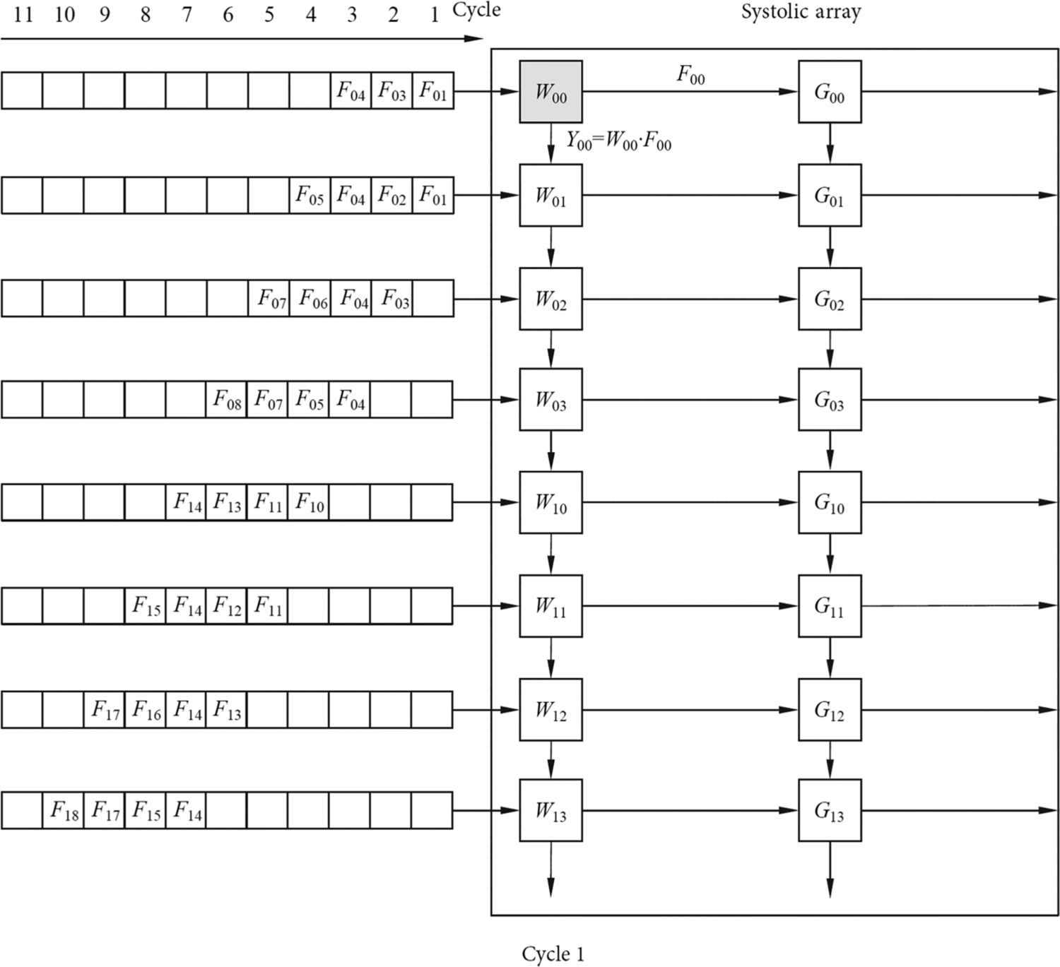
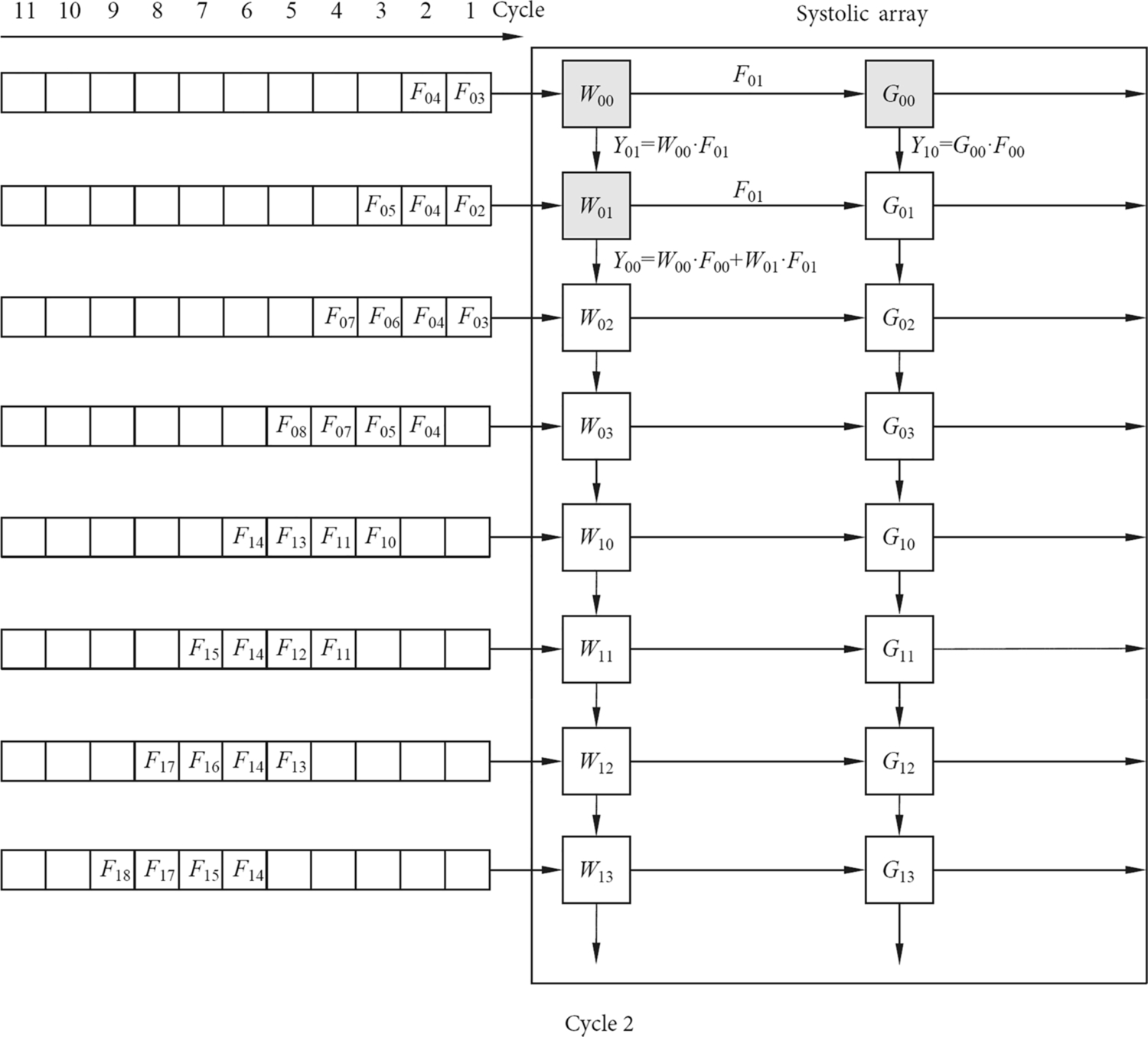
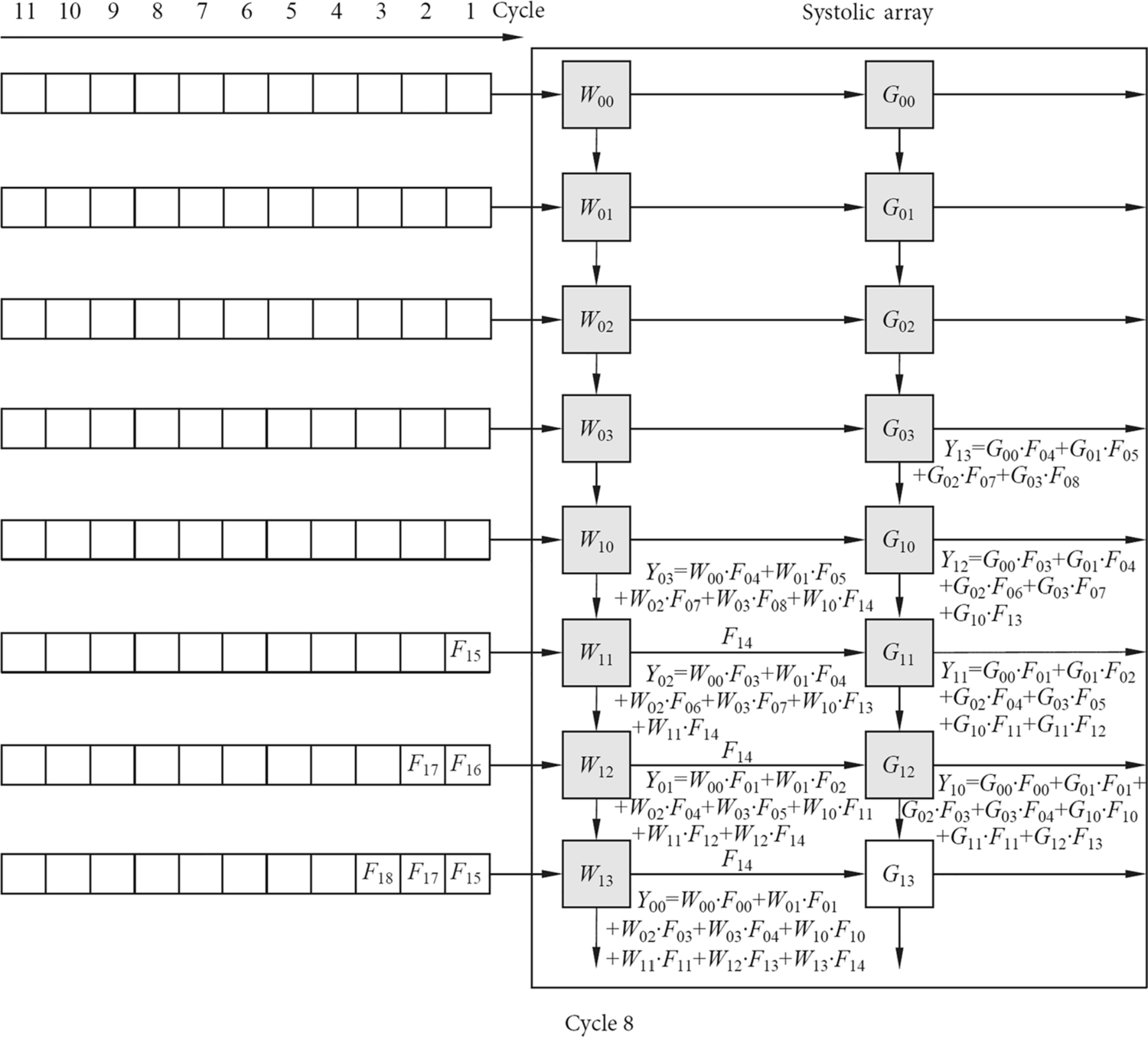
The state of the entire systolic array is shown in Fig. 2.7. When convolving with the two-channel input feature matrix F and the convolution kernels W and G, F is first re-arranged and loaded through the data loader into the leftmost column of the systolic array. The input data go from top to bottom, and each row entering the systolic array is delayed by one clock cycle from the previous row. In the first clock cycle, the input data F00 enters the W00 multiply-add unit and the multiply-add operation with W00 yields the unit result Y00, which is the first partial sum of Y00. In the second clock cycle, as shown in Fig. 2.8, the partial sum of the last W00 multiply-add unit Y00 is passed down to the W01 multiply-add unit, while the second row of the input value F01 is multiplied by W01 and added to the second partial sum of the Y00. On the other hand, F01 enters the W00 multiply-add unit and performs multiplication and addition to obtain the first partial sum of Y01. At the same time, F00 slides to the right and enters the G00 multiply-add unit to obtain the first partial sum of the unit result Y10.
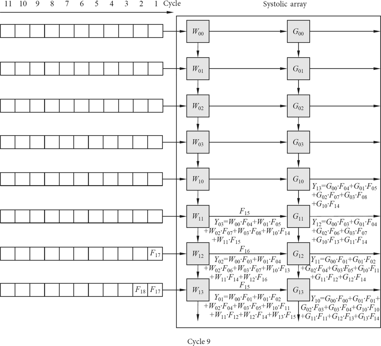
Similarly, the data of the input feature matrix are continuously slid to the right along the horizontal direction of the systolic array to produce the partial sums of the different convolution kernels. In the meantime, the partial sums corresponding to each convolution kernel continuously slide down to the vertical direction of the column of the systolic array and accumulate with the result of the current multiply-add units, thereby obtaining the final convolution results for all channels of the convolution kernel in the lowermost computation unit of each column. As shown in Fig. 2.9, the first convolution result is obtained at the end of the eighth clock cycle. As shown in Fig. 2.10, after the ninth clock cycle, two results can be obtained each time. The convolution operation is not completed until all input data are convolved. The systolic array transfers data by simultaneous systolic in both directions, and the input data enters the array in a stepwise manner, and the final convolution results of each convolution kernel is sequentially generated.
The characteristics of the systolic array determine that the data must be fed sequentially, so each time to fill the entire systolic array, certain startup time is needed, and the startup time often causes a waste of hardware resources. The startup time can be estimated using {row number + column number − 1} where column number and row number are sizes of the systolic array. When the startup time is passed, the entire systolic array becomes fully loaded, and the maximum throughput can be obtained.
The convolution results in the example of Figs. 2.6 are computed using fixed convolution kernel weights, with input data being fed through lateral systolic and partial sums being transferred through longitudinal systolic. Briefly speaking, we use fixed kernels and horizontally moving inputs and vertically moving partial sums. Actually, the same results can be obtained by fixing any one of the three and moving the other two. For example, we may fix the partial sums and horizontally move the inputs and vertically move the kernels. In practice, the selection of configurations will be determined based on the actual situation and application requirements.
It should be pointed out that when the convolution kernel is too large, there are too many channels, or if the weights of all channels are arranged in one column, it will inevitably cause the systolic array to be too large, which is not practical for the actual circuit design. To address this problem, split computation and accumulation are often used. The system divides the multichannel weight data into several blocks, each of which can fit the size of the systolic array. The weights of each block are then computed separately and sequentially, and the partial results of the computations are temporarily stored in a set of additive accumulators at the bottom of the systolic array. When the computation of a weights block finishes and the weight block is swapped with the next, the results are accumulated. After all the weight blocks are used, the accumulator accumulates all the results and outputs the final.
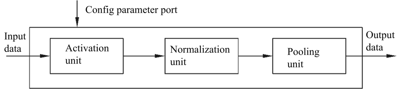
The systolic array in the TPU only performs the convolution operations, and the computation of the entire neural network requires the assistance of other computing units. As shown in Fig. 2.11, the vector computing unit receives the convolution results from the systolic array through the input data port and generates an activation value by a nonlinear function in the activation unit, and the activation function can be customized based on requirements. In the vector computing unit, the activation value can also be normalized and then pooled. These operations are controlled by the queue module. For example, the queue module can specify an activation function, a normalization function, or a pooling function, and can also configure parameters such as step size through a parameter configuration port. After the processing of the vector computing unit, the activation values are sent to the unified buffer for temporary storage and as the input of the next layer. In this way, the TPU is able to perform the computation of the whole neural network layer by layer.
Although the systolic array is mainly targeted on the acceleration of neural networks, the architecture can handle much more than convolution operations. It is also efficient and powerful for the general matrix operations, so it can be used for a range of tasks other than convolution neural networks, such as fully connected neural networks, linear regression, logistic regression, clustering (such as K-means clustering), video en −/decoding, and image processing.
2.2.2.2: Google TPU architecture
Google’s TPU processor, combined with its own TensorFlow software framework, can be used to accelerate the common algorithms for deep learning and has been successfully deployed to Google’s cloud computing platform. The TPU is an application-specific processor for neural networks (please refer to https://cloud.google.com/blog/products/gcp/an-in-depth-look-at-googles-first-tensor-processing-unit-tpu for TPU architecture). Its main architecture modules include systolic array, vector computing unit, main interface module, queue module, unified buffer (UB), and direct memory access (DMA) control module.
The main interface is used to obtain parameters and configurations of the neural network, such as network-layer number, weights, and other initial parameters. After receiving the read command, the DMA control module will read the input features and weight data and store them in the on-chip UB. At the same time, the main interface sends an instruction to start execution of the queue module. After receiving the instruction, the queue module starts and controls the runtime mode of the whole neural network, such as loading the weight and feature data into the systolic array, splitting the data into blocks, and performing the computation by blocks. The main function of the unified buffer is to store the intermediate results of the input and output, or to send the intermediate result to the systolic array for the operation of the next layer. The queue module can send control signals to the unified buffer, the systolic array, and the vector computing unit, or directly communicate with the DMA control module and the memory.
In general, when applying TPU for the training or inference of neural networks, it operates on each layer of network sequentially. The system first obtains the input values from the off-chip memory and sends them to the systolic array to efficiently perform the convolution or other matrix operations. The vector unit utilizes special hardware for nonlinear activation and pooling. The output of each layer can be temporarily saved in the unified buffer to be used as input to the next layer. The overall process is a pipeline that is executed in an orderly manner under the control of instructions and hardware state machines.
The first generation of the TPU is equipped with 65,536 8-bit multiply-add units (MACs), which can support unsigned and signed integers, but does not support floating-point operations. A total of 4 MB of accumulator buffer is distributed around the systolic array and supports 32-bit accumulation. All intermediate results can be stored using a unified buffer of 24 MB. The TPU has an external 8 GB memory and can store a large number of images and convolution kernel data.
The instructions executed by the TPU are transmitted through the PCIe bus. The instructions belong to the CISC instruction set. The average number of clock cycles required to complete each instruction is approximately 10–20. Most of the instructions of the TPU belong to macros, which are essentially state machines controlled by hardware. This has the advantage of greatly reducing the overhead caused by instruction decoding and storage. The TPU has five main instructions for neural networks: data read instruction (Read_Host_Memory), weight read instruction (Read_Weight), matrix operation instruction (MatrixMultiply/Convolve, Activate), and data write back instruction (Write_Host_Memory). A complete instruction accounts for 12 bits in total, in which the unified buffer address accounts for 3 bits, the accumulator buffer address accounts for 2 bits, the operand length accounts for 4 bits, and the remaining 3 bits are the opcode and flag bits.
The basic instruction execution flow of the TPU is: first, the input feature data or image data are read from the system memory into the unified buffer by the Read_Host_Memory instruction; then the convolution kernel weight is extracted from the memory by the Read_Weight instruction and fed into the systolic array as part of the input of the systolic array; the function of the instruction MatrixMultiply/Convolve is to send the input data in the unified buffer to the systolic array based on certain rules and then load the results into the accumulator buffer for accumulation; then execute the Activate command to perform nonlinear activation functions, normalization and pooling by using the vector computing unit, and the results are stored in the unified buffer. Finally, the Write_Host_Memory instruction is used to write the final result of the completion in the unified buffer back into system memory.
2.3: Deep learning framework
With the popularity of deep learning, a variety of software frameworks has emerged. These frameworks are mostly open-source, and each of them has attracted many advocates in a short time. The main goal of these frameworks is to free deep learning researchers from tedious and detailed programming work, so their main focus can be on the tuning and improvement of AI algorithms. Since deep learning algorithms change rapidly and more and more hardware platforms begin supporting deep learning, the popularity of a framework often depends on how broad the ecosystem is and how well the framework can implement state-of-the-art algorithms while best exploiting the underlying hardware architectures.
2.3.1: MindSpore
MindSpore is a next-generation deep learning framework launched by Huawei originating from industry best practices [14]. It combines the computing power of the AI processor, supports flexible deployment of edge and cloud applications, and creates a new AI programming paradigm that simplifies the development of AI applications.
In the “Huawei CONNECT Conference” of 2018, ten challenges faced by artificial intelligence were put forward. Key among them was that algorithm training time was up to days or even months, that computing power was scarce and expensive, and that costs were prohibitive. Another issue was that AI still faced the challenge that there was no “intelligence” without considerable “manual” labor for practitioners with advanced skills to collect and label data. To date, the high technology threshold, high development cost, long deployment cycle, and other issues have hindered the development of industry-wide ecosystems. To help developers and industry more coherently address those systemic challenges, Huawei’s next-generation artificial intelligence framework MindSpore focuses on simple programming with easy debugging, yet which yields high performance and flexible deployment options to effectively lower the development threshold. The details are as follows.
- (1) Programming in MindSpore is simple. As shown in Code 2.1, MindSpore introduces a new paradigm for AI programming. It incorporates an innovative functional differential programming architecture that allows data scientists to focus on the mathematical representation of model algorithms. The operator-level automatic differentiation technology makes it unnecessary to manually implement and test the inverse operator when developing a new network, reducing the effort required to deliver cutting-edge scientific research.
- (2) MindSpore is easy to debug. MindSpore provides a GUI which enables an easier debugging experience. It also provides both dynamic and static development and debugging modes where lines of code or a statement allows developers to switch the debugging mode. As shown in Code 2.2, when high-frequency debugging is required, the dynamic graph mode is selected, and the single operator/subgraph is executed to facilitate development and debugging. When it is required to run efficiently, it can be switched to the static graph mode which is compiled and executed using advanced optimization.
- (3) MindSpore offers excellent performance. MindSpore executes models through AI Native which maximizes computing power across device, edge, and cloud platforms. Utilizing Huawei’s AI processor for local execution, efficient data format processing, deep graph optimization, and other characteristics helps to achieve maximum performance, in turn helping developers to reduce training time and improve inference performance. As the datasets and models of modern deep neural networks get bigger and bigger, the memory and computing power of the single machine cannot meet the demands placed on it leading to a need for model parallelism. Manually partitioning tasks is slow and challenging to debug. As shown in Code 2.3, MindSpore automates model segmentation and tuning through flexible policy definition and cost models leading to optimal efficiency and performance.
- (4) MindSpore has flexible deployment options. MindSpore provides consistent development across all platforms, facilitates on-demand collaboration between platforms and enables flexible deployment letting developers quickly deploy mobile, edge-to-cloud AI applications in all scenarios that achieve higher efficiency and unmatched privacy protection. MindSpore is open-source and scalable, which improves the prosperity of artificial intelligence and enables developers to flexibly extend third-party frameworks and third-party hardware for their needs. MindSpore provides sufficient tutorials and guides on the portal and open-source communities.
2.3.2: Caffe
In early neural network research, researchers needed to develop programs for heterogeneous architectures such as CPUs and GPUs in order to carry out and accelerate large-scale neural network operations. This required programmers to have advanced programming skills and a deep understanding of programming environments such as CUDA. Such requirements have severely impeded the development and promotion of deep learning. In 2012, AlexNet made waves in deep learning research with large-scale training and 10 × performance improvement by using GPUs [15]. This prompted the development of many deep learning frameworks, often developed by global technology giants, including the most representative of them: the open-source framework, Caffe [16].
Caffe (Convolutional Architecture for Fast Feature Embedding) was created by Jia Yangqing during his PhD at the University of California at Berkeley based on C ++/Cuda, and subsequently adapted to Python with PyCaffe. Caffe performs computations on either CPU or GPU with developers only defining the structure and parameter configuration of neural networks. Command-line options control either efficient training or inference of networks. In addition, Caffe also supports the development of customized network layers. Developers only need to implement layer parsing, feed-forward, and back-propagation functions of a layer to support new functionality. Debugging of programs and porting between different systems very easy since Caffe is based on C ++. Lastly, Caffe provides a number of pretrained models that enable researchers to perform rapid iterative studies on neural networks by modifying parameters or fine-tuning the network based on pretrained models. For these reasons, Caffe stood out in the early days of the deep learning.
In the Caffe framework, structure and parameters of a neural network are defined by a prototxt file. Prototxt is the Google Protocol Buffer library (protobuf) for storing text. It is a lightweight and efficient structured data storage format that can be used for structured data serialization. It is very suitable for data storage or RPC data exchange, like JSON or XML but more efficient. The three most important concepts in protobuf are the proto file, the prototxt file, and the protoc compiler.
The proto file is used to define the organization of the data and is mainly composed of a package name (PackageName) and a message definition (MessageDefinition). Code 2.4 shows a definition of a proto file, where syntax specifies the protobuf version, package specifies the namespace, message defines a message type that contains multiple field definitions, and the field can be Required, Optional, and Repeatable, and the type of the field can be a common Int32, Double, String, or an enumerated type. Caffe source code defines caffe.proto itself to define various message types used internally. The most important ones are LayerParameter for defining layer parameters, SolverParameter for defining solver parameters and NetParameter for defining network structure.
The prototxt file is a text file that is serialized according to the format defined in the proto file. There is also a corresponding binary file, but the text file is easier to read and modify. Caffe’s prototxt file contains two types of information: one is to define the neural network structure and the other is to define the training network parameters. The data structure in the prototxt file defining the neural network structure is defined by NetParameter, where “layer” represents each layer in the neural network, the structure of which is defined by the LayerParameter. As shown in Code 2.5, a prototxt representing a neural network structure can have multiple layers, depending on which parameters are used to determine the type of layer, parameters, and connections between them. Caffe builds the structure of the neural network by parsing the prototxt file. In addition, network training parameters used by Caffe optimizers such as learning rate are defined in the prototxt files. After parsing this information, Caffe is able to train the network.
During Caffe compilation, the protoc compiler compiles caffe.proto to get caffe.pb.cc and caffe.pb.h, which contain the serialization and deserialization interfaces for all defined message types. Caffe can use these interfaces to generate or parse all message types defined by caffe.proto. For example, through the LayerParameter definition, each layer in the prototxt file can be parsed into a LayerParameter class, which is further passed according to the parsed type field. Subclasses of the corresponding LayerParameter class, such as ConvolutionParameter, parse specific layer parameters. Code 2.6 shows an example of a concrete maximum pooling layer whose format follows the LayerParameter definition, where the pooling_param field format follows the PoolingParameter definition.
In the Caffe framework, the intermediate feature map data is usually arranged in a four-dimensional array, called a Blob, and its specific format is defined in caffe.proto. Input image data needs to be stored in either lmdb or leveldb database format. The corresponding path of dataset and information are stored in prototxt through DataParameter. Currently, caffe also supports direct reading of image data through OpenCV [17] although this requires the OpenCV library and a separate ImageDataParameter.
After compiling Caffe, you can control the corresponding inference and training process merely through the command line, and the corresponding commands are as follows. As shown in Code 2.7, Caffe is a compiled executable program that requires only the solver file for training. The inference requires the prototxt file of the neural network and the corresponding weight file.
Since Caffe is written in C ++, the structure of the library is clear: each layer has a special C ++ implementation as well as a Cuda implementation for GPUs. This allows users to easily develop their own models in Caffe and is a large part of why Caffe is still widely used by major companies and universities for algorithm research and application deployment. Developing a customized layer in Caffe generally requires the following steps:
- (1) add information defining the parameters of the customized layer, LayerParameter in caffe.proto;
- (2) inherit Caffe built-in classes, build customized layer classes, provide methods for parameter parsing, memory allocation, shape calculation, layer registration, etc. This step provides providing the most important feed-forward and back-propagation implementations on CPU and GPU;
- (3) write a test file, recompile Caffe, and the customized layer is added successfully if no error is reported;
- (4) modify the prototxt file for training and inference.
The original Caffe is no longer updated and has been gradually replaced by Caffe2 since the original framework supports only single-GPU computing, and does not support distributed training among other drawbacks such as model level parallelism. In spite of this, Caffe provides an efficient and convenient learning platform for many beginners in the development of deep learning and is often their first step into deep learning.
2.3.3: TensorFlow
TensorFlow is Google’s second-generation open-source deep learning framework [18]. It is based on DistBelief which was originally developed by GoogleBrain team for Google research and development. Released under the Apache 2.0 open-source license on November 9, 2015, it supports running on CPU, GPU, and Google’s own TPU. TensorFlow is currently the most widespread and widely used open-source framework in the deep learning community.
After AlphaGo defeated Lee Sedol, the top professional chess player, Google used the opportunity to launch TensorFlow, gaining support from many developers. This is in large part due to Google sparing no effort in developing and promoting TensorFlow by maintaining a quick update schedule, complete documentation, wide platform support, and a rich interface, particularly for Python. TensorFlow also supports a wide range of neural networks so that developers can quickly build cutting-edge applications without reinventing the wheel is also appreciated by many users.
TensorFlow’s name comes from its own operating principle. Tensor refers to the storage and transfer format of data between nodes in TensorFlow which are similar to arrays in NumPy library but different in many ways. Flow refers to the flow of tensor data. Input data flows as tensors through layers eventually flowing to the output node like a water stream after which the output data is obtained. TensorFlow abstracts network into simple data-flow diagrams that allow users to build models flexibly, without having to care about the underlying hardware scheduling or computational implementation details. By defining the computational graph in this manner, TensorFlow can further optimize the computational graph including operations such as memory allocation, data rearrangement, and so on. TensorFlow also supports distributed computing which may involve communication between different devices, unlike Caffe.
Although TensorFlow is a Python library, the computational graph formalism brings a completely different programming style. Typical Python libraries often provide a set of variables, functions, and classes. Using these libraries feels similar to writing normal Python code. However, when using TensorFlow, users find that the code used to define the computational graph in TensorFlow cannot be debugged or printed, and they even cannot use Python’s If-else and While statements.
This is because TensorFlow is essentially a new domain-specific language (DSL) based on Declarative programming. Users need first define the computational graph need run by TensorFlow. The computational graph has inputs, outputs, and the mapping between them, which is equivalent to defining a new program. This programming concept is called Metaprogramming which sounds very complex and difficult to understand. However, this concept will be elaborated upon later in this book to teach readers how to use it. For now, to develop a neural network program using TensorFlow, just follow these steps:
- (1) define the computational graph using the interfaces provided by TensorFlow;
- (2) read data using normal Python code;
- (3) provide data to the computational graph, run the computational graph, and get the output.
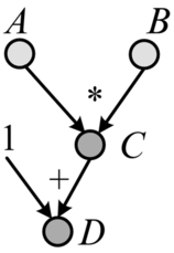
Taking the computation graph in Fig. 2.12 as an example, both A and B are arrays of shape {10}. After the Element-Wise Product, an array C of shape {10} is obtained, and then after adding another scalar, an array D of the same shape {10} is obtained. The corresponding TensorFlow code for this example is shown in Code 2.8.
The first concept of TensorFlow programming is the computational graph. Each TensorFlow program will build a computational graph by default, so the declaration of the graph is not explicitly displayed in the code. TensorFlow can define multiple computational graphs by tf.Graph, but there will only be one default computational graph at any time.
The second concept of TensorFlow programming is Nodes. Nodes may be compute nodes or data nodes. Compute nodes define a specific computation. In Code 2.8, tf.add defines tensor addition, and tf.multiply defines tensor multiplication. In addition, more high-level compute nodes like convolution, fully connected computation, and so on are equivalent to the layers defined in Caffe. The other type of node is data nodes. In Code 2.8, tf.placeholder in the above code defines a placeholder node which acts as an input to the computational graph. Other types of data nodes, like (1)tf.constant: defines constant nodes (2) tf.Variable: defines variables. Trainable parameters, such as weights, offsets, and so on are represented in the form of data nodes.
The third concept of TensorFlow programming is Tensor, which represents actual data in TensorFlow. It is reflected in the computational graph as the connection between nodes. In Code 2.8, A, B, C, and D are all tensor objects. There are two types of tensors: one is the tensor corresponding to placeholder output and is used to provide input data at runtime. The other is the tensor passed between compute nodes. When the user runs the computational graph TensorFlow computes the minimum dependency graph between inputs and outputs and uses this reduced graph to compute the output value(s).
The fourth concept of TensorFlow programming is the Session. It provides context for the computation of the entire computational graph, including configuration information for the GPU, etc.
2.3.4: PyTorch
PyTorch is a deep learning framework launched by Facebook in October 2016 [19]. It is an open-source Python machine learning library based on Torch. The official version was launched on December 7, 2018. It is very popular as Google’s TenosrFlow.
PyTorch is a second-generation deep learning framework like TensorFlow, but has some distinctive features. Although PyTorch is also based on a computational graph mechanism it feels very similar to ordinary Python code. This is because PyTorch uses Imperative Programming to dynamically generate graphs.
Each time a line of code is executed, the system constructs a corresponding computational graph and data is calculated in real-time. Such a computational graph is called a dynamic graph. In contrast, TensorFlow can only obtain data by running an existing computational graph. Such a computational graph is called a static graph. There is an animation on PyTorch’s GitHub official website that explains how it works. Interested readers can check it out.
Why does PyTorch, which introduces dynamic graphs, not count as a new generation of deep learning frameworks compared to TensorFlow? This is because the introduction of “dynamic graphs” in essence is only a change of user interface and interaction. Such flexibility is partly at the expense of runtime performance, and it cannot be regarded as true technological innovation. In fact, static graph based frameworks like TensorFlow are also introducing dynamic graphing mechanisms such as TensorFlow Eager and MxNet Gluon.
But in any case, imperative programming and dynamic graphing mechanisms make it easier for users to carry out deep learning development and programming. For example, recursive neural network and word2vec, which are challenging in TensorFlow, can be implemented easily with PyTorch.
Implementing the computations in Code 2.8, using PyTorch in Code 2.9 is much simpler and more similar to the typical Python code.
2.4: Deep learning compilation framework—TVM
With the introduction of many new deep learning frameworks and the emergence of an increasing number of hardware products, researchers in the field of deep learning have found that it is not easy to handle end-to-end software deployment and execution perfectly and efficiently. Although frameworks such as TensorFlow can support a variety of hardware such as CPU, GPU, and TPU, the migration of algorithm models among different deep learning frameworks (such as PyTorch, TensorFlow, and Caffe) is difficult. As shown in the left half of Fig. 2.13, different software programming methods and frameworks have different implementations on different hardware architectures, such as mobile phones, embedded devices, or servers in data centers. These factors increase the user’s costs.
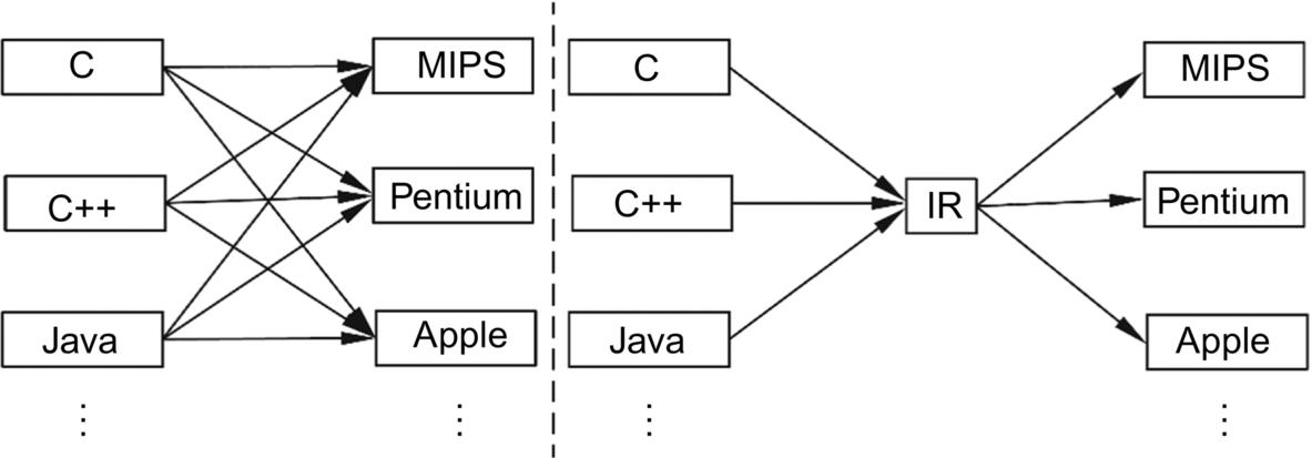
The compiler-level intermediate representation framework LLVM [20] solves this problem by setting up an intermediate instruction representation (IR), as shown in the right half of Fig. 2.14. All software frameworks are not directly mapped to specific hardware but are first compiled into an intermediate format of instruction representation by a front-end compiler. For specific hardware, the vendor can provide a back-end compiler that bridges the intermediate instructions and the specific hardware instructions, and implements the IR with the specific hardware instructions.
Motivated by this idea, a number of intermediate representations, compilers, and actuators dedicated to deep learning have emerged over the past few years. These are collectively referred to as a Compiler Stack. For example, nGraph proposed by Microsoft and SystemML published by IBM, and the TVM (Tensor Virtual Machine) framework proposed by Tianqi Chen’s team of University of Washington [21].
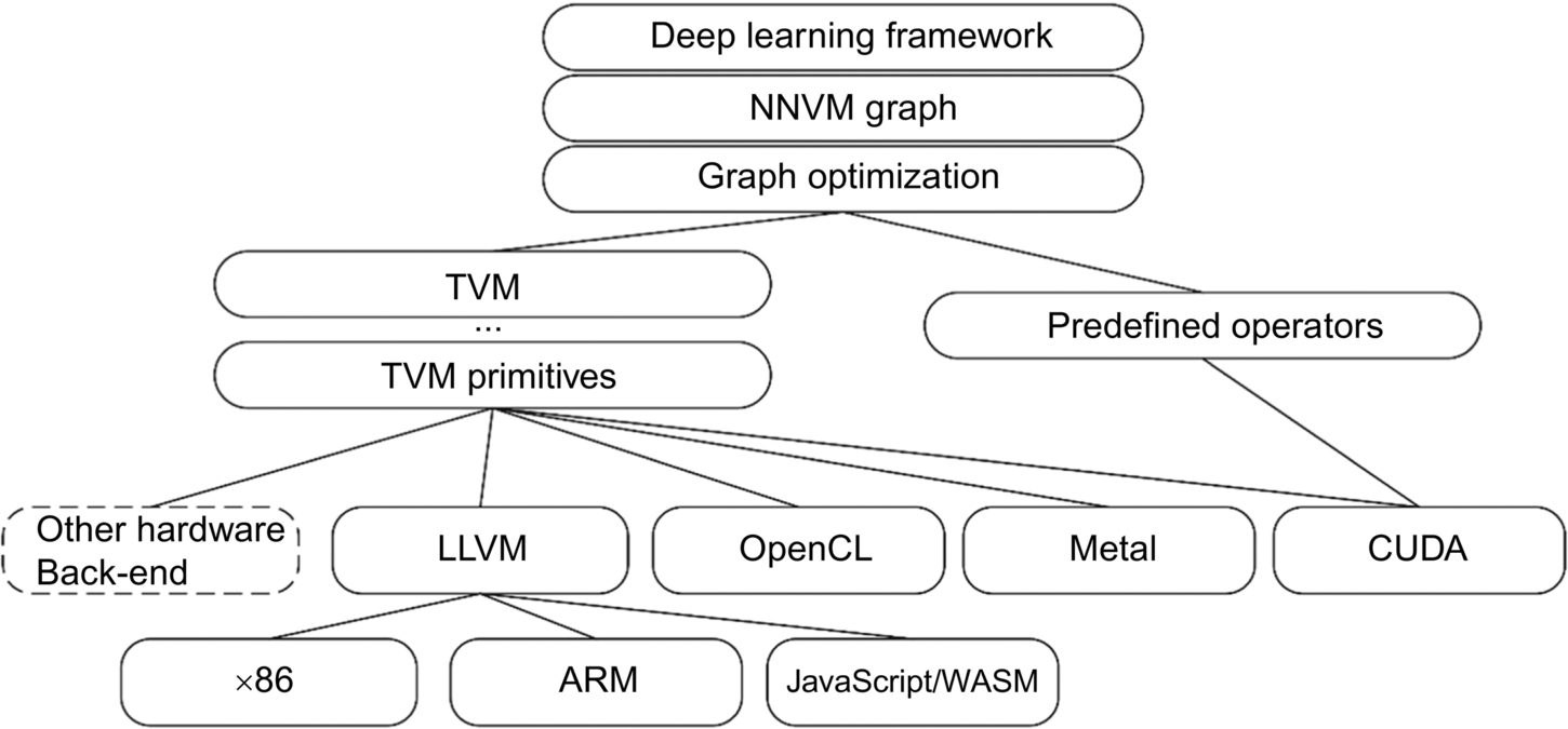
More details about TVM will be introduced in the following chapters but here is a brief introduction to the overall structure and major components. Similar to the LLVM framework, TVM is also divided into front-end, middle, and back-end. However, TVM introduces many additional features in the middle. As shown in Fig. 2.14, TVM provides the following functionalities:
- (1) converts computational graph representations of different frameworks into a unified NNVM intermedia representation (IR), and then perform graph-level optimizations upon the intermediate representations, such as operator fusion;
- (2) provides tensor-level intermediate representation (or TVM primitives), which separates the computing from the scheduling. It allows the implementation of different scheduling methods for the same operator on different hardware architectures; and
- (3) provides a learning-based optimization method that finds optimal scheduling methods within search space then quickly and automatically generates kernels whose performance can exceed those produced by manual optimization.
TVM’s contribution is not only to provide a set of compiler stacks that translate from the deep learning framework to the underlying hardware but more importantly to propose the abstractions from graph-level to operator-level by dividing the graph into primitive operations, combining the operators when needed and providing specific scheduling for each architecture. This enables users to use TVM to automatically or semiautomatically generate code or kernels that exceeds the performance of handwritten code. It greatly improves the efficiency of the development of high-performance deep learning applications.