
Applications: Acoustics and Psychoacoustics Combined
Chapter Contents
7.1 Critical Listening Room Design
7.1.1 Loudspeaker arrangements for critical listening
7.1.3 Energy–time considerations
7.1.4 Reflection-controlled rooms
7.1.5 The absorption level required for reflection-free zones
7.1.6 The absorption position for reflection-free zones
7.1.8 The diffuse reflection room
7.2 Pure-Tone and Speech Audiometry
7.3.1 Psychoacoustic experimental design issues
7.3.2 Psychoacoustic rating scales
7.3.3 Speech intelligibility: Articulation loss
7.4 Filtering and Equalization
7.4.1 Equalization and tone controls
7.4.2 Correcting frequency response faults due to the recording process
7.4.3 Timbre modification of sound sources
7.4.4 Altering the balance of sounds in mixes
7.5.2 The effect of reverberation on intelligibility
7.5.3 The effect of more than one loudspeaker on intelligibility
7.5.4 The effect of noise on intelligibility
7.5.5 Requirements for good speech intelligibility
7.5.6 Achieving speaker directivity
7.5.7 A design example: How to get it right
7.5.8 More than one loudspeaker and delays
7.5.9 Objective methods for measuring speech quality
7.7 “Mosquito” Units and “Teen Buzz” Ring Tones
7.8.1 The archetypical audio coder
7.8.2 What exactly is information?
7.8.3 The signal redundancy removal stage
7.8.4 The entropy coding stage
7.8.5 How do we measure information?
7.8.6 How do we measure the total information?
7.8.8 The psychoacoustic quantization stage
7.8.9 Quantization and adaptive quantization
7.8.10 Psychoacoustic noise shaping
7.8.11 Psychoacoustic quantization
So far in this book we have considered acoustics and psychoacoustics as separate topics. However, real applications often require the combination of the two because although the psychoacoustics tells us how we might perceive the sound, we need the acoustic description of sound to help create physical, or electronic, solutions to the problem. The purpose of this chapter is to give the reader a flavor of the many applications that make use of acoustics and psychoacoustics in combination. Of necessity these vignettes are brief and do not cover all the possible applications. However, we have tried to cover areas that we feel are important, and of interest. The level of detail also varies but, in all cases, we have tried to provide enough detail for the reader to be able to read, and understand, the more advanced texts and references that we provide, and any that the reader may discover themselves, for further reading. The rest of this chapter will cover listening room design, audiometry, psychoacoustic testing, filtering and equalization, public address systems, noise reducing headphones, acoustical social control devices, and last, but by no means least, audio coding systems.
7.1 Critical Listening Room Design
Although designing rooms for music performance is important, we often listen to recorded sound in small spaces. We listen to music, and watch television and movies, in both stereo and surround, in rooms that are much smaller that the recording environments. If one wishes to evaluate the sound in these environments then it is necessary to make them suitable for this purpose. In Chapter 6 we have seen how to analyze existing rooms and predict their performance. We have also examined methods for improving their acoustic characteristics. However, is there anything else we can do to make rooms better for the purpose of critically listening to music? There are a variety of approaches to achieving this and this section examines: optimal speaker placement, IEC rooms, room energy evolution, LEDE rooms, non-environment rooms, and diffuse reflection rooms.
7.1.1 Loudspeaker Arrangements for Critical Listening
Before we examine specific room designs, let us first examine the optimum speaker layouts for both stereo and 5.1 surround systems. The reason for doing this is that most modern room designs for critical listening need to know where the speakers will be in order to be designed. It is also pretty pointless having a wonderful room if the speakers are not in an optimum arrangement.
Figure 7.1 shows the optimum layout for stereo speakers. They should form an equilateral triangle with the center of the listening position. If one has a greater angle than this the center phantom image becomes unstable—the so-called “hole in the middle” effect. Clearly, having an angle of less than 60° results in a narrower stereo image.

Figure 7.1 Optimal stereo speaker layout.
5.1 surround systems are used in film and video presentations. Here the objective is to provide both clear dialog and stereo music and sound effects, as well as a sense of ambience. The typical speaker layout is shown in Figure 7.2. Here, in addition to the conventional stereo speakers there are some additional ones to provide the additional requirements. These are as follows:

Figure 7.2 Typical speaker layout for 5.1 surround.
- Center dialog speaker: The dialog is replayed via a central speaker because this has been found to give better speech intelligibility over a stereo presentation. Interestingly the fact that the speech is not in stereo is not noticeable because the visual cue dominates so that we hear the sound coming from the person speaking on the screen even if their sound is coming from a different direction.
- Surround speakers: The ambient sounds, and sound effects, are diffused via rear mounted speakers. However they are, in the main, not supposed to provide directional effects and so are often deliberately designed, and fed signals, to minimize their correlation with each other and the front speakers. The effect of this is to fool the hearing system into perceiving the sound as all around with no specific direction.
- Low-frequency effects: This is required because many of the sound effects used in film and video, such as explosions and punches, have substantial low-frequency and subsonic content. Thus, a specialized speaker is needed to reproduce these sounds properly. Note: this speaker was never intended to reproduce music signals, notwithstanding their presence in many surround music systems.
More recently systems using six or more channels have also been proposed and implemented; for more information see Rumsey (2001).
As we shall see later the physical arrangement of loudspeakers can significantly affect the listening room design.
7.1.2 IEC Listening Rooms
The first type of critical listening room is the IEC listening room (IEC, 2003). This is essentially a conventional room that meets certain minimum requirements: a reverberation time that is flat, and between 0.3 and 0.6 seconds above 200 Hz, a low noise level, an even mode distribution and a recommended floor area. In essence this is a standardized living room that provides a consistent reference environment for a variety of listening tasks. It is the type of room that is often used for psychoacoustic testing as it provides results that correlate well with that which is experienced in conventional domestic environments. This type of room can be readily designed using the techniques discussed in Chapter 6.
However, for critically listening to music mixes, etc. something more is required and these types of room will now be discussed. All of them don’t only control reverberation, but also the time evolution and level of early reflections. They also all take advantage of the fact that the speakers are in specific locations to do this and very often have an asymmetric acoustic that is different for the listener and the loudspeakers. Although there are many different implementations, they fall into three basic types: reflection controlled rooms, non-environment rooms, and diffuse reflection rooms. As they all control the early reflections within a room we shall look at them first.
7.1.3 Energy–Time Considerations
A major advance in acoustical design for listening to music has arisen from the realization that, as well as reverberation time, the time evolution of the first part of the sound energy build-up in the room matters, that is, the detailed structure and level of the early reflections, as discussed in Chapter 6. As it is mostly the energy in the sound that is important as regards perception, the detailed evolution of the sound energy as a function of time in a room matters. Also there are now acoustic measurement systems that can measure the energy-time curve of a room directly, thus allowing a designer to see what is happening within the room at different frequencies, rather than relying on a pair of “golden ears.” An idealized energy–time curve for a typical room is shown in Figure 7.3. It has three major features:

Figure 7.3 An idealized energy–time curve.
- A gap between the direct sound and first reflections. This happens naturally in most spaces and gives a cue as to the size of the space. The gap should not be too long—less than 30 ms—or the early reflections will be perceived as echoes. Some delay, however, is desirable as it gives some space for the direct sound and so improves the clarity of the sound, but a shorter gap does add “intimacy” to the space.
- The presence of high-level diffuse early reflections, which come to the listener predominantly from the side, that is, lateral early reflections. This adds spaciousness and is easier to achieve over the whole audience in a shoebox hall rather than a fan-shaped one. The first early reflections should ideally arrive at the listener within 20 ms of the direct sound. The frequency response of these early reflections should ideally be flat and this, in conjunction with the need for a high level of lateral reflections, implies that the side walls of a hall should be diffuse reflecting surfaces with minimal absorption.
- A smoothly decaying diffuse reverberant field which has no obvious defects, and no modal behavior, and whose time of decay is appropriate to the style of music being performed. This is hard to achieve in practice so a compromise is necessary in most cases. For performing acoustic music a gentle bass rise in the reverberant field is desirable to add “warmth” to the sound but in studios this is less desirable.
7.1.4 Reflection-Controlled Rooms
For the home listener, or sound engineer in the control room of a studio, the ideal would be an acoustic that allows them to “listen through” the system to the original acoustical environment that the sound was recorded in. Unfortunately the room in which the recorded sound is being listened to is usually much smaller than the original space and this has the effect shown in Figure 7.4. Here the first reflection the listener hears is due to the wall in the listening room and not the acoustic space of the sound that has been recorded. Because of the precedence effect this reflection dominates, and the replayed sound is perceived as coming from a space the size of the listening room, which is clearly undesirable. What is required is a means of making the sound from the loudspeakers appear as if it is coming from a larger space by suppressing the early reflections from the nearby walls, as shown in Figure 7.5. Examples of this approach are: “live end dead end” (LEDE) (Davies and Davies, 1980), “Reflection free zone” (RFZ) (D’Antonio and Konnert, 1984), and controlled reflection rooms (Walker, 1993, 1998).

Figure 7.4 The effect of a shorter initial time delay gap in the listening room.

Figure 7.5 Maximizing the initial time delay by suppressing early reflections.
One way of achieving this is to use absorption, as shown in Figure 7.6. The effect can also be achieved by using angled or shaped walls, as shown in Figures 7.7 and 7.8. This is known as the “controlled reflection technique” because it relies on the suppression of early reflections in a particular area of the room to achieve a larger initial time delay gap. This effect can only be achieved over a limited volume of the room unless the room is made anechoic, which is undesirable. The idea is simple: by absorbing, or reflecting away, the first reflections from all walls except the furthest one away from the speakers the initial time delay gap is maximized. If this gap is larger than the initial time delay gap in the original recording space then the listener will hear the original space, and not the listening room.

Figure 7.6 Achieving a reflection-free zone using absorption.
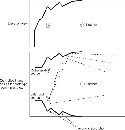
Figure 7.7 Controlled reflection room (in the style of Bob Walker) for free-standing loudspeakers (from Newell 2008).

Figure 7.8 An example controlled reflection room, Sony Music M1, New York, NY. (Photo by Paul Ellis of The M Network Ltd; Acoustician: Harris, Grant Associates)
However, this must be achieved while satisfying the need for even diffuse reverberation, and so the rear wall in such situations must have some explicit form of diffusion structure on it to assure this. The initial time delay gap in the listening should be as large as possible, but is clearly limited by the time it takes sound to get to the rear wall and back to the listener. Ideally this gap should be 20 ms but it should not be much greater or it will be perceived as an echo. In most practical rooms this requirement is automatically satisfied and initial time delay gaps in the range of 8 ms to 20 ms are achieved.
Note that if the reflections are redirected rather than being absorbed, then there will be “hot areas” in the room where the level of early reflections is higher than normal. In general it is often architecturally easier to use absorption rather than redirection, although this can sometimes result in a room with a shorter reverberation time.
7.1.5 The Absorption Level Required for Reflection-Free Zones
In order to achieve a reflection-free zone it is necessary to suppress early reflections, but by how much? Figure 7.9 shows a graph of the average level that an early reflection has to be at in order to disturb the direction of a stereo image. From this we can see that the level of the reflections must be less than about 15 dB to be subjectively inaudible. Allowing for some reduction due to the inverse square law, this implies that there must be about 10 dB, or α = 0.9 of absorption on the surfaces contributing to the first reflections. In a domestic setting it is possible to get close to the desired target using carpets and curtains, and bookcases can form effective diffusers, although persuading the other occupants of the house that carpets, or curtains, on the ceiling is chic can be difficult. In a studio more extreme treatments can be used. However, it is important to realize that the overall acoustic must still be good and comfortable, that it is not anechoic, and that, due to the wavelength range of audible sound, this technique is only applicable at mid to high frequencies where small patches of treatment are significant with respect to the wavelength.

Figure 7.9 The degree of reflection suppression required to assure a reflection-free zone (data from Toole, 1990).
7.1.6 The Absorption Position for Reflection-Free Zones
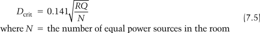
Figure 7.10 shows one method of working out where absorption should be placed in a room to control early reflections. By imagining the relevant walls to be mirrors it is possible to create “image rooms” that show the direction of the early reflections. By defining a reflection-free space around the listening position, and by drawing “rays” from the image speaker sources, one can see which portions of the wall need to be made absorbent, as shown in Figure 7.11. This is very straightforward for rectangular rooms, but a little more complicated for rooms with angled walls. Nevertheless, this technique, can still be used. It is applicable for both stereo and surround systems, the only real difference being the number of sources.
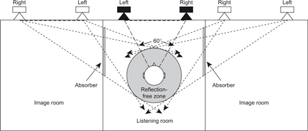
Figure 7.10 The image method for controlled reflection room absorption placement.

Figure 7.11 Non-environment room principles.
In Figure 7.11 the rear wall is not treated because normally some form of diffusing material would be placed there. However, absorbing material could be so placed, in the places determined by another image room created by the rear wall, if these reflections were to be suppressed. One advantage of this technique is that it also shows places where absorption is unnecessary. This is useful because it shows you where to place doors and windows that are difficult to make absorptive. To minimize the amount of absorption needed one should make the listening area as small as possible because larger reflection free volumes require larger absorption patches. The method is equally applicable in the vertical as well as the horizontal direction.
7.1.7 Non-Environment Rooms
Another approach to controlling early reflections, which is used in many successful control rooms, is the “non-environment” room. These rooms control both the early reflections and the reverberation. However, although they are quite dead acoustically, they are not anechoic. Because for users in the room there are some reflections from the hard surfaces, there are some early reflections that make the room non-anechoic. However, sound that is emitted from the speakers is absorbed and is never able to contribute to the reverberant field. How this is achieved is shown in Figure 7.11.
These rooms have speakers, which are flush mounted in a reflecting wall, and a reflecting floor. The rear wall is highly absorbent, as are the side walls and ceiling. The combined effect of these treatments is that sound from the loudspeakers is absorbed instead of being reflected so that only the direct sound is heard by the listener, except for a floor reflection. However, the presence of two reflecting surfaces does support some early reflections for sources away from the speakers. This means that the acoustic environment for people in the room, although dead, is not oppressively anechoic. Proponents of this style of room say that the lack of anything but the direct sound makes it much easier to hear low-level detail in the reproduced audio and provides excellent stereo imaging. This is almost certainly due to the removal of any conflicting cues in the sound, as the floor reflection has very little effect on the stereo image.
These rooms require wide-band absorbers as shown in Figure 7.12. These absorbers can take up a considerable amount of space. As one can see in Figure 7.12, the absorbers can occupy more than 50% of the volume. However, it is possible to use wide-band membrane absorbers, as discussed in Chapter 6, with a structure similar to that shown in Figure 6.48 with a limp membrane in place of the perforated sheet. Using this type of absorber it is possible to achieve sufficient wide-band absorption with a depth of 30 cm, which allows this technique to be applied in much smaller rooms whose area is approximately 15 m2. Figure 7.13 shows a typical non-environment room implementation: “The Lab”, at the Liverpool Music House

Figure 7.12 A non-environment control room. Shaded areas are wide-band absorbers (from Newell, 2008)

Figure 7.13 A non-environment room implementation: “The Lab” at the Liverpool Music House (from Newell, 2008).
Because non-environment rooms have no reverberant field, there is no reverberant room support for the loudspeaker level, as discussed in Section 6.1.7. Only the direct sound is available to provide sound level. In a normal domestic environment, as discussed in Chapter 6, the reverberant field is providing most of the sound power and is often about 10 dB greater than the direct sound. Thus in a non-environment room one must use either 10 times the power amplifier level, or specialist loudspeaker systems with a greater efficiency, to reproduce the necessary sound levels (Newell, 2008).
7.1.8 The Diffuse Reflection Room
A novel approach to controlling early reflections is not to try to suppress or redirect them, but instead diffuse them. This results in a reduced reflection level but does not absorb them.
In general most surfaces absorb some of the sound energy and so the reflection is weakened by the reflection. Therefore the level of direct reflections will be less than that which would be predicted by the inverse square law, due to surface absorption. The amount of energy, or power, removed by a given area of absorbing material will depend on the energy, or power, per unit area striking it. As the sound intensity is a measure of the power per unit area this means that the intensity of the sound reflected is reduced in proportion to the absorption coefficient. Therefore the intensity of the early reflection is given by:
![]()
From the above equation (7.1), which is Equation 1.18 with the addition of the effect of surface absorption, it is clear that the intensity reduction of a specular early reflection is inversely proportional to the distance squared.
Diffuse surfaces on the other hand scatter sound in other directions than the specular. In the case of an ideal diffuser the scattered energy polar pattern would be in the form of a hemisphere. A simple approach to calculating the effect of this can be to model the scattered energy as a source whose initial intensity is given by the incident energy. Thus, for an ideal scatterer, the intensity of the reflection is give by the product of the equation describing the intensity from the source and the one describing the sound intensity radiated by the diffuser. For the geometry shown in Figure 7.14 this is given by:

Figure 7.14 The geometry for calculating the intensity of an early reflection from a diffuse surface.

The factor 2 in the second term represents the fact that diffuser only radiates into half a hemisphere and therefore has a “Q” of 2. From Equation 7.2 one can see that the intensity of a diffuse reflection is inversely proportional to the distance to the power of four. This means that the intensity of an individual diffuse reflection will be much smaller than that of a specular reflection from the same position.
So diffusion can result in a reduction of the amplitude of the early reflection from a given point. However, there will also be more reflections, due to the diffusion, arriving at the listening position from other points on the wall, as shown in Figure 7.15. Surely this negates any advantage of the technique? A closer inspection of Figure 7.15 reveals that although there are many reflection paths to the listening point they are all of different lengths, and hence time delay. The extra paths are also all of a greater length than the specular path, shown dashed in Figure 7.15. Furthermore the phase reflection diffusion structure will add an additional temporal spread to the reflections. As a consequence the initial time delay gap will be filled with a dense set of low-level early reflections instead of a sparse set of higher level ones, as shown in Figure 7.16. Of particular note is that, even with no added absorption, the diffuse reflection levels are low enough in amplitude to have no effect on the stereo image, as shown earlier in Figure 7.9.

Figure 7.15 Additional early reflection paths due to a diffuse surface.

Figure 7.16 The intensity–time plots at the listener position of a diffuser walled room compared with the direct sound.
The effect of this is a large reduction of the comb filtering effects that high-level early reflections cause. This is due to both the reduction in amplitude due to the diffusion and the smoothing of the comb filtering caused by the multiplicity of time delays present in the sound arriving from the diffuser. As these comb filtering effects are thought to be responsible for perturbations of the stereo image (Rodgers, 1981), one should expect improved performance even if the level of the early reflections is slightly higher than the ideal.
The fact that the reflections are diffuse also results in an absence of focusing effects away from the optimum listening position and this should result in a more gradual degradation of the listening environment away from the optimum listening position. Figure 7.17 shows the intensity of the largest diffuse side wall reflection relative to the largest specular side wall reflection as a function of room position for the speaker position shown. From this figure we can see that over a large part of the room the reflections are less than 15 dB below the direct sound.

Figure 7.17 The intensity of the largest diffuse side wall reflection relative to the direct sound as a function of room position; contours are in dB relative to the direct sound.
Figure 7.18 shows one of the few examples of such a room. The experience of this room is that one is unaware of sound reflection from the walls: it sounds almost anechoic, yet it has reverberation. Stereo and multi-channel material played in this room has images that are stable over a wide listening area, as predicted by theory. The room is also good for recording in as the high level of diffuse reflections and the acoustic mixing it engenders, as shown in Figure 7.15, helps to integrate the sound emitted by acoustic instruments.

Figure 7.18 A diffuse reflection room implementation: “Studio C,” at Blackbird Studio, Nashville. (Photo by Max Crace courtesy of George Massenburg and Blackbird Studio.)
Summary
In this section we have examined various techniques for achieving a good acoustic environment for hearing both stereo and multi-channel music. However, the design of a practical critical listening room requires many detailed considerations regarding room treatment, sound isolation, air conditioning, etc. that are covered in more detail in Newell (2008).
7.2 Pure-Tone and Speech Audiometry
In this section, a number of acoustic and psychoacoustic principles are applied to the clinical measurement of hearing ability. Hearing ability is described in Chapter 2 and summarized in Figure 2.10 in terms of the frequency and amplitude range typically found. But how can these be measured in practice, particularly in the clinic where such information can provide medical professionals with critical data for the treatment of hearing problems?
The ability to detect sound and the ability to discriminate between sounds are the two aspects of hearing that can be detrimentally affected by age, disease, trauma or noise-induced hearing loss. The clinical tests that are available for the diagnosis of these are:
- Sound detection: pure-tone audiometry.
- Sound discrimination: speech audiometry.
Pure-tone audiometry is used to test a subject’s hearing threshold at specific frequencies approximately covering the speech hearing range (see Figure 2.10). These frequencies are spaced in octaves as follows: 125 Hz, 250 Hz, 500 Hz, 1 kHz, 2 kHz, 4 kHz and 8 kHz. The range of sound levels that are tested usually start 10 dB below the average threshold of hearing and they can rise to 120 dB above it; recall that the average threshold of hearing varies with frequency (see Figure 2.10).
A clinical audiometer is set up to make diagnosis straightforward, and quick and easy to explain to patients. Because the threshold of hearing is a non-uniform curve and therefore not an easy reference to use on an everyday basis in practice, a straight line equating to the average threshold of hearing is used instead to display the results of a hearing test on an audiogram. A dBHL (hearing level) scale is defined for hearing testing, which is the number of dBs above the average threshold of hearing.
Figure 7.19 shows a blank audiogram which plots frequency on the x axis (the octave values between 125 Hz and 8 kHz inclusive as shown above) against dBHL between −10 dBHL and +120 dBHL on the y axis. Note that the dBHL scale increases downwards to indicate greater hearing loss (a higher amplitude or greater dBHL value needed for the sound to be detected). The 0 dBHL (threshold of hearing) line is thicker than the other lines to give a visual focus on the average threshold of hearing as a reference against which measurements can be compared.

Figure 7.19 A blank audiogram.
A pure-tone audiometer has three main controls: (1) frequency; (2) output sound level; and (3) a spring-loaded output key switch to present the sound to the subject. When the frequency is set, the level is automatically altered to take account of the average threshold of hearing, which enables the output sound level control to be calibrated in dBHL directly. The output sound level control usually works in 5 dB steps and is calibrated in dBHL. It is vitally important that the operator is aware that an audiometer can produce very high sound levels which could do permanent damage to a normal hearing system (see Section 2.5). When testing a subject’s hearing, a modest level around + 30 dBHL should be used to start with, which can be increased if the subject cannot hear it.
The spring-loaded output key is used to present the sound, thereby giving the operator control of when the sound is being presented and removing any pattern of presentation that might allow the subject to predict when to expect the next sound. Such unpredictability adds to the overall power of the test, but, in the context of hearing measurement, it is particularly important when hearing is being tested in the context of, at one extreme, a legal claim for damages being made for hearing loss due to noise-induced hearing loss or, at the other, a health screening for normal hearing as part of a job interview.
When a sound is heard the subject is asked to press a button, which illuminates a lamp, or light emitting diode (LED), on the front panel of the audiometer. The subject should be visible to the tester, but the subject should not be able to see the controls. When carrying out an audiometric test, local sound levels should be below the levels defined in BS EN ISO 8253-1, which are shown for the test frequencies in Figure 7.20. Generally, the local level should be below 35 dBA.

Figure 7.20 Local maximum sound levels at audiometric test frequencies for acoustic and bone conduction measurements (adapted from BS EN ISO 8253-1).
During audiometry, test signals are presented in one of two ways:
- air conduction
- bone conduction.
For air conduction audiometry, sound is presented acoustically to the outer ear and thereby tests the complete hearing system. Three types of air conduction transducers are available:
circum-aural headphones
supra-aural headphones
ear canal insert earphones.
Circum-aural headphones surround and cover the pinna (see Figure 2.1) completely thereby providing a degree of sound isolation. Supra-aural headphones rest on the pinna and are the more traditional type in use, but they are not particularly comfortable since they press quite heavily on the pinna in order to keep the distance between the transducer itself and the tympanic membrane constant. Both circum- or supra-aural headphones can be uncomfortable and somewhat awkward and they can in certain circumstances deform the ear canal. As an alternative, ear canal insert earphones that have a disposable foam tip can be used which will not distort the ear canal. They have the added advantage that less sound leaks to the other ear, which reduces the need to consider presenting a masking signal to it. There are, however, situations, such as infected or obstructed ear canals, when the use of ear canal insert earphones is not appropriate.
For bone conduction audiometry, sound is presented mechanically using a bone vibrator which is placed just behind but not touching the pinna on the bone protrusion known as the “mastoid prominence.” It is held in place with an elastic headband. The sound presented when using bone conduction bypasses the outer and middle ears since it vibrates the temporal bone in which the cochlea lies directly. Thus it can be used to assess inner function and the presence or otherwise of what is known as “sensorineural hearing loss” with no hindrance from any outer or middle ear disorder. Bone conduction is carried out in the same way as air conduction audiometry except that only frequencies from 500 Hz to 4 kHz are used due to the limitations of the bone conduction transducers themselves. When a bone conduction measurement is being made for a specific ear it is essential that the other ear is masked using noise. Specific audiometric guidelines exist for the use of masking.
The usual audiometric procedure for air or bone conduction measurements (recalling the one difference for bone conduction that the frequencies used are from 500 Hz to 4 kHz only) is to test frequencies (in the following order: 1 kHz, 1 kHz, 2 kHz, 4 kHz, 8 kHz, 500 Hz, 250 Hz, 125 Hz, 1 kHz). (Note that the starting frequency is 1 kHz which is a mid frequency in the hearing range and is therefore likely to be heard by all subjects to give them confidence at the start and end of a test.) If the retest measurement at 1 kHz has changed by more than 5 dB, other frequencies should be retested and the most sensitive value (lowest dBHL value) recorded. When testing one ear, consideration will be given as to whether masking should be presented to the other ear to ensure that only the test ear is involved in the trial. This is especially important when testing the poorer ear.
Tests are started at a level that can be readily heard (usually around +30 dBHL), which is presented for 1–3s using the output key switch, and then involve watching for the subject to light the lamp or LED. If this does not happen, the level is increased in 5 dB steps (5 dB being a minimum practical value to enable tests to be carried out in a reasonable time)—presenting the sound and awaiting a response each time. Once a starting level has been established, the sound level is changed using the “10 down, 5 up” method as follows:
Reduce the level in 10 dB steps until the sound is not heard.
Increase the level in 5 dB steps until the sound is heard.
Repeat 1 and 2 until the subject responds at the same level at least 50% of the time, defined as two out of two, two out of three or two out of four responses.
Record the threshold as the lowest level heard.
There are a number of degrees of hearing loss, which are defined in Table 7.1. These descriptions are used to provide a general conclusion about a subject’s hearing and they should be interpreted as such. They consist of a single value which is the average dBHL value across frequencies 250 Hz to 4 kHz. The values are used to provide a general guideline as to the state of hearing and it must be remembered that there could be one or more frequencies for which the hearing loss is worse than the average.
Table 7.1 Definitions of different degrees of hearing loss
| Description | dBHL |
No hearing handicap | <20 |
Mild hearing loss | 20–40 |
Moderate hearing loss | 41–70 |
Severe hearing loss | 71–95 |
Profound hearing loss | >95 |
Consider, for example, the audiogram for damaged hearing given in Figure 2.19. Here, the average dBHL value for frequencies 250 Hz to 4 kHz would be {((10 + 5 + 5 + 15 + 60)/5) = 19 dBHL} which indicates “no hearing handicap” (see Table 7.1), which is clearly not the case.
The upper part of Figure 7.21 shows audiograms for a young adult with normal healthy hearing within both ears based on air and bone conduction tests in the left and right ears (a key to the symbols used on audiograms is given in the figure). Notice that the bone and air conduction results lie in the same region (in this case <20 dBHL) and a summary statement of “no hearing handicap” (see Table 7.1) would be entirely appropriate in this case. Pure-tone audiometry is the technique that enables the normal deterioration of hearing with age, or presbycusis (see Section 2.3 and Figure 2.11) to be monitored.

Figure 7.21 UPPER: Example audiograms for the left and right ears (left- and right-hand plots respectively) of a young adult with normal healthy hearing along with a key to the symbols commonly used on audiograms. LOWER: Example audiograms for (left) a left ear conductive hearing loss, and (right) a right ear hearing loss due to congenital rubella syndrome.
The lower part of Figure 7.21 shows example audiograms for two hearing loss conditions. The audiogram in the lower left position shows a conductive hearing loss in the left ear because the bone conduction plot is normal, but the air conduction plot shows a significant hearing loss that would be termed a “moderate hearing loss” (see Table 7.1). This indicates a problem between the outside world and the inner ear, and a hearing aid, tailored to the audiogram, could be used to correct for the air conduction loss.
The audiogram in the lower right position shows the effect on hearing of congenital rubella syndrome which can occur in a developing fetus of a pregnant woman who contracts rubella (German measles) from about 4 weeks before conception to 20 weeks into pregnancy. One possible effect on the infant is profound hearing loss (>95 dBHL—see Table 7.1), which is sensorineural (note that both the air and bone conduction results lie in the same region indicating an inner ear hearing loss). Sadly, there is no known cure; in this example, a hearing aid would not offer much help because there is no usable residual hearing above around 500 Hz.
Pure-tone audiometry tests a subject’s ability to detect different frequencies, and the dBHL values indicate the extent to which the subject’s hearing is reduced at different frequencies. It thus indicates those frequency regions in which a subject is perhaps less sensitive than normally hearing listeners. This could, for example, be interpreted in practice in terms of timbral differences between specific musical sounds that might not be heard, or vowel or other speech sounds that might be difficult to perceive. However, pure-tone audiometry does not provide a complete test of a subject’s hearing ability to discriminate between different sounds. Discrimination of sounds does start with the ability to detect the sounds, but it also requires appropriate sound processing to be available. For example, if the critical bands (see Section 2.2) are widened, they are less able to separate the components of complex sounds—the most important to us being speech. In order to test hearing discrimination, speech audiometry is employed which makes use of spoken material.
Speech audiometry is carried out for each ear separately and tests speech discrimination performance against the pure-tone audiograms for each ear and normative data. When testing one ear, consideration will be given as to whether masking should be presented to the other ear to ensure that only the test ear is involved in the trial. This is particularly important when testing the poorer ear.
Speech audiometry involves the use of an audiometer and speech material that is usually recorded on audio compact disc (CD). Individual single syllable words such as bus, fun, shop are played to the subject, who is asked to repeat them, providing part words if that is all they have heard. Each spoken response is scored phonetically in terms of the number of correct sounds in the response (for example, if bun or boss was the response for bus, the subject would score two out of three). Words are presented in sets of 10, and if a total phonetic score of 10% or better is achieved for a list, the level is reduced by 10 dB and a new set of 10 words is played, repeating the process until the score falls below 10%. The Speech Reception Threshold (SRT) is the lowest level at which a 10% phonetic score can be achieved. The Speech Discrimination Score (SDS) is the percentage of single syllable words that can be identified at a comfortable loudness level.
The results from speech audiometry indicate something about the ability to discriminate between sounds whereas pure-tone audiometry indicates ability to detect the presence of particular frequency components. Clearly detection ability is basic to being able to make use of frequency components in a particular sound, but how a listener might make use of those components depends on their discrimination ability. Discrimination will change if, for example, a listener’s critical bands are widened, which can result in an inability to separate individual components. This could have a direct effect on pitch, timbre and loudness perception. In addition, the ability to hear separately different instruments or voices in an ensemble might be impaired—something that could be very debilitating for a conductor, accompanist or recording engineer.
7.3 Psychoacoustic Testing
Knowledge of psychoacoustics is based on listening tests in order to find out how humans perceive sounds in terms, for example, of pitch, loudness and timbre. Direct measurements are not possible in this context since direct connections cannot be made for ethical as well as practical reasons, and, in many cases, there is a cognitive dimension (higher-level processing) that is unique to each and every listener. Our knowledge of psychoacoustics therefore is based on listening tests, and this section presents an overview of procedures that are typically used in practice. Apart from offering this as a background to the origins of the psychoacoustic information presented in this book, it also enables readers to think through aspects of the creation of their own listening tests to progress psychoacoustic knowledge in the future.
When carrying out a psychoacoustic test, it is important to note that the responses will be from the opinions of listeners; that is, they will be subjective, whereas an objective test involves a direct physical measurement such as dB SPL, Hz, or spectral components. There is no right answer to a subjective test since it is the opinion of a particular listener and each listener will have an opinion that is unique; the process of psychoacoustic testing is to collect these listener opinions in a non-judgmental manner. Subjective testing is unlike objective testing where direct measurements can be made of physical quantities such as sound pressure level, sound intensity level or fundamental frequency; in a subjective test a listener is asked to offer an opinion in answer to questions such as “Which sound is louder?”, “Does the pitch rise or fall?”, “Are these two sounds the same or different?”, “Which chord is more in-tune?”, or “Which version do you prefer?”.
Psychoacoustic testing involves careful experimental design to ensure that the results obtained can be truly attributed to whatever aspect of the signal is being used as the controlled variable. This process is called controlled experimentation. A starting point for experimental design may well be a hunch or something we believe to be the case from our own listening experience, or from anecdotal evidence. A controlled experiment allows such listening experiences to be carefully explored in terms of which aspects of a sound affect them and how. Psychologists call a behavioral response, such as a listening experience, the dependent variable, and those aspects that might affect it are called the independent variables. Properly controlled psychoacoustic testing involves controlling all the independent variables so that any effects observed can be attributed to changes in the specific independent variable under test.
7.3.1 Psychoacoustic Experimental Design Issues
One experimental example might be to explore what aspects of sound affect the perception of pitch. The main dependent variable would be f0, but other aspects of sound can affect the perceived pitch such as loudness, timbre and duration (see Section 3.2). Experimentally, it would also be very appropriate to consider other issues that might affect the results—some of which may not initially seem obvious—such as the fact that hearing abilities of the subjects can vary with age (see Section 2.3) and general health, or that perhaps subjects’ hearing should be tested (see Section 7.2).
The way in which sounds are presented to subjects can also make a difference since the use of loudspeakers would mean that the acoustics of the room will alter the signals arriving at each ear (see Chapter 6) whereas the use of headphones would not. There may be background acoustic noise in the listening room that could affect the results and this may even be localized, perhaps to a ventilation outlet. Subjects can become tired (listener fatigue), distracted, or may perform better at different times of the day. The order in which stimuli are presented can have an effect—perhaps of alerting the listener to specific features of the signal, which prepares them better for a following stimulus. These are all potential independent variables and would need proper controlling.
Part of the process of planning a controlled experiment is thinking through such aspects (the ones given here are just examples and are not presented as a definitive list) before carrying out a full test. It is common to try a pilot test with a small number of listeners to check the test procedure and for the presence of any additional independent variables. Some independent variables can be controlled by ensuring they remain constant (for example, the ventilation might be turned off, and measures could be taken to reduce background noise). Others can be controlled through the test procedure (for example, any learning effect could be explored by playing the stimuli in a different order to different subjects or asking each listener to take the test twice with the stimulus order being reversed the second time).
7.3.2 Psychoacoustic Rating Scales
For many psychoacoustic experiments the request to be given to the listeners is straightforward. In the pitch example above one might ask listeners to indicate which of two stimuli has the highest pitch or whether the pitch of a single stimulus was changing or not. In experiments where the objective is to establish the nature of change in a sound, such as whether one synthetic sound is more natural than another, it is not so easy. A simple “yes” or “no” would not be very informative since it would not indicate the nature of the difference. A number of rating scales have been produced that are commonly used in such cases, where the listener is invited to choose the point on the scale that best describes what they have heard. Some examples are given below.
When speech signals are rated subjectively by listeners, perhaps for the evaluation of the signal provided by a mobile phone or the output from a speech synthesis system, it is usually the quality of the signal that is of interest. The number of listeners is important since each will have a personal opinion and it is generally suggested that at least 16 are used to ensure that statistical analysis of the results is sufficiently powerful. However, the greater the number of listeners the more reliable the results are. It is also most appropriate to use listeners who are potential users of whatever system might result from the work and listeners who are definitely not experts in the area. A number of rating scales exist for the evaluation of the quality of a speech signal and the following are examples:
- absolute category-rating (ACR) test;
- degradation category-rating (DCR) test;
- comparison category-rating (CCR) test.
The absolute category-rating (ACR) test requires listeners to respond with a rating from the five-point ACR rating scale shown in Table 7.2. The results from all the listeners are averaged to provide a mean opinion score (MOS) for the signals under test. Depending on the purpose of the test, it might be of more interest to present the results of the listening test in terms of the percentage of listeners that rated the presented sounds in one of the categories such as good or excellent or poor or bad.
A comparison is requested of listeners in a degradation category-rating (DCR) test, and this usually involves a comparison between a signal before and after some form of processing has been carried out. The assumption here is that the processing is going to degrade the original signal in some way, for example after some sort of coding scheme such as MP3 (see Section 7.8) has been applied, where one would never expect the signal to be improved. Listeners use the DCR rating scale (see Table 7.2) to evaluate the extent to which the processing has degraded the signal when comparing the processed version with the unprocessed original. The results are analyzed in the same way as for the ACR test and these are sometimes referred to as the “degradation mean opinion score” (DMOS).
Table 7.2 Rating scale and descriptions for the absolute category-rating (ACR) test, which produces a mean opinion score (MOS), and degradation category-rating (DCR) test, which produces a degraded mean opinion score (DMOS)
| Rating | ACR description – MOS | DCR description – DMOS |
5 | Excellent | Degradation not perceived |
4 | Good | Degradation perceived but not annoying |
3 | Fair | Degradation slightly annoying |
2 | Poor | Degradation annoying |
1 | Bad | Degradation very annoying |
In situations where the processed signal could be evaluated as being either better or worse, a comparison category-rating (CCR) test can be used. Its rating scale is shown in Table 7.3 and it can be seen that it is a symmetric two-sided scale. Listeners are asked to rate the two signals presented in terms of the quality of the second signal relative to the first. The CCR test might be used if one is interested in the effect of a signal processing methodology being applied to an audio signal, such as noise reduction, in terms of whether it has improved the original signal or not.
Table 7.3 Rating scale and descriptions for the comparison category-rating (CCR) test
| Rating | Description |
3 | Much better |
2 | Better |
1 | Slightly better |
0 | About the same |
−1 | Slightly worse |
−2 | Worse |
−3 | Much worse |
7.3.3 Speech Intelligibility: Articulation Loss
Psychoacoustic experiments may be used to define thresholds of perception and rating scales for small degradations, such as the quality of the sound. However, at the other end of the quality scale is the case where the degradation, due to noise distortion, reverberation, etc., is so severe that it affects the intelligibility of speech. This is also measured and defined by the results of psychoacoustic experiments, but in these circumstances, instead of annoyance, the dependent variable is the proportion of the words that are actually heard correctly.
Two parameters are found to be important by those who work on speech: the “intelligibility” and the “quality,” or “naturalness,” of the speech. Both reflect human perception of the speech itself, and while they are most directly measured subjectively with panels of human listeners, research is being carried out to make equivalent objective measurements of these, because of the problems of setting up listening experiments and the inherent inter- and intra-listener variability. The relationship between intelligibility and naturalness is not fully understood. Speech that is unintelligible would usually be judged as being unnatural. However, muffled, fast or mumbling speech is natural, but less intelligible, and speech that is highly intelligible may or may not be unnatural.
Subjective measures of intelligibility are often based on the use of lists of words that rhyme, differing only in their initial consonant. In a diagnostic rhyme test (DRT), listeners fill in the leading consonants on listening to the speech, and often the possible consonants will be indicated. In a modified rhyme test (MRT) each test consists of a pair-wise comparison of acoustically close initial consonants such as feel–veal, bowl–dole, fought–thought, pot–tot. The DRT identifies quite clearly in what area a speech system is failing, giving the designers guidance on where they might make modifications. DRT tests are widely accepted for testing intelligibility, mainly because they are rigorous, accurate and repeatable. Another type of testing is “Logatom” testing.
In Logatom testing nonsense words such as “shesh” and “bik” are placed into a carrier phrase such as “Can con buy <Logatom, e.g., “shesh” here> also.” to ensure that they are all pronounced with the same inflection. The listener then has to identify the nonsense word and write it down. Using nonsense words has the advantage of removing the higher language processing that we use to resolve words with degraded quality and so provides a less biased measure. The errors listeners make show how the system being tested damages the speech, such as particular letter confusions, and provide a measure of intelligibility. Typically lists of 50 or 100 Logatoms are used as a compromise between accuracy and fatigue, as discussed earlier. Although in theory any consonant-vowel-consonant may be used, it has been the authors’ experience that rude or swear words must be excluded, because the talker usually cannot pronounce them with the same inflection as normal words.
All of these tests result in a measure of the number of correctly identified words. This, as a percentage of the total, can be used as a measure of intelligibility, or articulation loss, respectively. As consonants are more important in Western languages than vowels, this measure is often focused on just the consonants to form a measure called %ALcons (Articulation Loss; consonants) which is the percentage of consonants that are heard incorrectly. If this is greater than 15% then the intelligibility is considered to be poor. Although articulation loss is specific to speech—an important part of our auditory world—much music also relies on good articulation for its effect.
Subjective testing is a complex subject and could fill a complete book just by itself! For more details see Bech and Zacharov (2006).
7.4 Filtering and Equalization
One of the simplest forms of electronic signal processing is to filter the signal in order to remove unwanted components. For example, often low-frequency noises, such as ventilation and traffic rumble, need to be removed from the signal picked up by the microphone. A high-pass filter would accomplish this and mixing desks often provide some form of high-pass filtering for this reason. High frequencies also often need to be removed to either ameliorate the effects of noise and distortion or remove the high-frequency components that would cause alias distortion in digital systems. This is achieved via the use of a low-pass filter. A third type of filter is the notch filter, which is often used to remove tonal interference from signals. Figure 7.22 shows the effect of these different types of filter on the spectrum of a typical music signal.

Figure 7.22 Types of filter and their effect.
In these cases the ideal would be to filter the signal in a way that minimized any unwanted subjective effect on the desired signal. Ideally, in these cases the timbre of the sound being processed should not change after filtering, but in practice there will be some effects. What are these effects and how can they be minimized in the light of acoustic and psychoacoustic knowledge?
The first way of minimizing the effect is to recognize that many musical instruments do not cover the whole of the audible frequency range. Few instruments have a fundamental frequency that extends to the lowest frequency in the audible range and many of them do not produce harmonics or components that extend to the upper frequencies of the audible range. Therefore, in theory one can filter these instruments such that only the frequencies present are passed with no audible effect. In practice this is not easily achieved for two reasons:
- Filter shape: Real filters do not suddenly stop passing signal components at a given frequency. Instead there is a transition from passing the signal components to attenuating them, as shown in Figure 7.23. The cut-off frequency of a filter is usually expressed as the point at which it is attenuating the signal by 3 dB relative to the pass-band; see Figure 7.23. Thus if a filter’s cut-off is set to a given frequency there will be a region within the pass-band that affects the amplitude of the frequency components of the signal. This region can extend as far as an octave away from the cut-off point. Therefore, in practice, the filter’s cut-off frequency must be set beyond the pass-band that one would expect from a simple consideration of the frequency range of the instruments, in order to avoid any tonal change due to change in frequency content caused by the filter’s transition region. As the order of the filter increases, both the slope of the attenuation as a function of frequency and the sharpness of the cut-off increase; this reduces the transition region effects, but unfortunately increases the time domain effects.
- Time domain effects: Filters also have a response in the time domain. Any form of filtering which reduces the bandwidth of the signal will also spread it over a longer period of time. In most practical filter circuits these time domain effects are most pronounced near the cut-off frequency and become worse as the cut-off becomes sharper. Again, as in the case of filter shape, these effects can extend well into the pass-band of the filter. Note that even the notch filter has a time response, which gets longer as the notch bandwidth reduces. Interestingly, particular methods of digital filtering are particularly bad in this respect because they result in time domain artifacts that precede the main signal in their output. These artifacts are easily unmasked and so become subjectively disturbing. Again, the effect is to require that the filter cut-off be set beyond the value that one would expect from a simple consideration of the frequency range of the instruments.

Figure 7.23 The specifications of a real filter.
Because of these effects the design of filters that achieve the required filtering effect without subjectively altering the timbre of the signal is difficult.
The second way of minimizing the subjective effects is to recognize that the ear uses the spectral shape as a cue to timbre. Therefore the effect of removing some frequency components by filtering may be partially compensated by enhancing the amplitudes of the frequency components nearby, as discussed in Chapter 5. Note that this is a limited effect and cannot be carried too far. Figure 7.24 shows how a filter shape might be modified to provide some compensation. Here a small amount of boost, between 1 dB and 2 dB, has been added to the region just before cut-off in order to enhance the amplitude of the frequencies near to those that have been removed.

Figure 7.24 Partially compensating for filtered components with a small boost at the bandedge.
7.4.1 Equalization and Tone Controls
A related, and important, area of signal processing to filtering is equalization. Unlike filtering, equalization is not interested in removing frequency components but in selectively boosting, cutting or reducing them to achieve a desired effect. The process of equalization can be modeled as a process of adding or subtracting a filtered version of the signal from the signal, as shown in Figure 7.25. Adding the filtered version gives a boost to the frequencies selected by the filter whereas subtracting the filtered output reduces the frequency component amplitudes in the filter’s frequency range. The filter can be a simple high- or low-pass filter, which results in a treble or bass tone control, or it can be a band-pass filter to give a bell-shaped response curve. The cut-off frequencies of the filters may be either fixed or variable depending on the implementation. In addition the bandwidths of the band-pass filters and, less commonly, the slopes of the high- and low-pass filters can be varied.
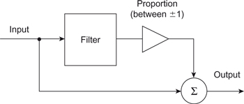
Figure 7.25 Block diagram of tone control function.
An equalizer in which all the filter’s parameters can be varied is called a parametric equalizer. However, in practice many implementations, especially those in mixing desks, only use a subset of the possible controls for both economy and simplicity of use. Typically in these cases, only the cut-off frequencies of the band-pass, and in some cases the low- and high-pass, filters are variable. There is an alternative version of the equalizer structure that uses a bank of closely spaced fixed frequency band-pass filters to cover the audio frequency range. This approach results in a device known as the “graphic equalizer” with typical bandwidths of the individual filters ranging from one-third of an octave to 1 octave. For parametric equalizers the bandwidths can become quite small.
Because a filter is required in an equalizer the latter also has the same time domain effects that filters have, as discussed earlier. This is particularly noticeable when narrow-bandwidth equalization is used, as the associated filter can “ring,” as shown in Figures 1.62 and 1.63, for a considerable length of time in both boost and cut modes.
Equalizers are used in three main contexts (discussed below) which each have different acoustic and psychoacoustic rationales.
7.4.2 Correcting Frequency Response Faults due to the Recording Process
This was one of the original functions of an equalizer in the early days of recording, which to some extent is no longer required because of the improvement in both electroacoustic and electronic technology. However, in many cases there are effects that need correction due to the acoustic environment and the placement of microphones. There are three common acoustic contexts that often require equalization:
- Close miking with a directional microphone: The acoustic bass response of a directional microphone increases, as it is moved close to an acoustic source, due to the proximity effect. This has the effect of making the recorded sound bass heavy; some vocalists often deliberately use this effect to improve their vocal sound. This effect can be compensated for by applying some bass-cut to the microphone signal and this often has the additional benefit of further reducing low-frequency environmental noises. Note that some microphones have this equalization built in but that in general a variable equalizer is required to fully compensate for the effect.
- Compensating for the directional characteristics of a microphone: Most practical microphones do not have an even response at all angles as a function of frequency. In general they become more directional as the frequency increases. As most microphones are designed to give a specified on-axis frequency response, in order to capture the direct sound accurately, this results in a response to the reverberant sound which falls with frequency. For recording contexts in which the direct sound dominates, for example close miking, this effect is not important. However, in recordings in which the reverberant field dominates, for example classical music recording, the effect is significant. Applying some high-frequency boost to the microphone signal can compensate for this.
- Compensating for the frequency characteristics of the reverberant field: In many performance spaces the reverberant field does not have a flat frequency response, as discussed in Section 6.1.7, and therefore subjectively colors the perceived sound if distant miking is used. Typically the bass response of the reverberant field rises more than is ideal, resulting in a bass heavy recording. Again the use of some bass-cut can help to reduce this effect. However, if the reverberation is longer at other frequencies, for example in the midrange, then the reduction should be applied in a way that complements the increase in sound level this causes. As in these cases the bandwidth of the level rise may vary, this must also be compensated for—usually by adjusting the bandwidth, or “Q,” of the equalizer.
All the above uses of equalization compensate for limitations imposed by the acoustics of the recording context. To make intelligent use of it in these contexts requires some idea of the likely effects of the acoustics of the space at a particular microphone location, especially in terms of the direct to reverberant sound balance.
7.4.3 Timbre Modification of Sound Sources
A major role for equalizers is the modification of the timbre of both acoustically and electronically generated sounds for artistic purposes. In this context the ability to boost or cut selected frequency ranges is used to modify the sounds spectrum to achieve a desired effect on its timbre. For example boosting selected high-frequency components can add “sparkle” to an instrument’s sound whereas adding a boost at low frequencies can add “weight” or “punch.” Equalizers achieve these effects through spectral modification only: they do not modify the envelope or dynamics of a music signal. Any alteration of the timbre is purely due to the modification, by the equalizer, of the long-term spectrum of the music signal. There is also a limit to how far these modifications can be carried before the result sounds odd, although in some cases this may be the desired effect.
When using equalizers to modify the timbre of a musical sound it is important to be careful to avoid “psychoacoustic fatigue”—this arises because the ear and brain adapt to sounds. This has the effect of dulling the effect of a given timbre modification over a period of time. Therefore one puts in yet more boost, which one adapts to, and so on. The only remedy for this condition is to take a break from listening to that particular sound for a while and then listen to it again later. Note that this effect can happen at normal listening levels and so is different to the temporary threshold shifts that happen at excessive sound levels.
7.4.4 Altering the Balance of Sounds in Mixes
The other major role is to alter the balance of sounds in mixes—in particular the placing of sound “up-front” or “back” in the mix. This is because the ability of the equalizer to modify particular frequency ranges can be used to make a particular sound become more or less masked by the sounds around it. This is similar to the way the singer’s formant is used to allow a singer to be heard above the orchestra as mentioned in Chapter 4. For example suppose one has a vocal line that is being buried by all the other instrumentation going on. The spectrum of such a situation is shown in Figure 7.26 and from this it is clear that the frequency components of the instruments are masking those of the vocals. By selectively reducing the frequency components of the instruments at around 1.5 kHz, while simultaneously boosting the components in the vocal line over the same frequency range, the frequency components of the vocal line can become unmasked, as shown in Figure 7.27. This has the subjective effect of bringing the vocal line out from the other instruments.
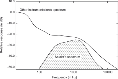
Figure 7.26 Spectrum of a masked soloist in the mix.

Figure 7.27 Spectrum after the use of equalization to unmask the soloist.
Similarly, performing the process in reverse would further reduce the audibility of the vocal line in the mix. To achieve this effect successfully requires the presence of frequency components of the desired sound within the frequency range of the equalizer’s boost and cut region. Thus different instruments require different boost and cut frequencies for this effect. Again it is important to apply the equalization gently in order to avoid substantial changes in the timbre of the sound sources.
Equalizers therefore have a broad application in the processing of sound. However, despite their utility, they must be used with caution—firstly to avoid extremes of sound character, unless that is desired, and secondly to avoid unwanted interactions between different equalizer frequency ranges. As a simple example consider the effect of adding treble, bass and midrange boost to a given signal. Because of the inevitable interaction between the equalizer frequency responses, the net effect is to have the same spectrum as the initial one after equalization. All that has happened is that the gain is higher. Note that this can happen if a particular frequency range is boosted and then, because the result is a little excessive, other frequency ranges are adjusted to compensate.
Sound reinforcement of speech is often taken for granted. However, as anyone who has tried to understand an announcement in a reverberant and noisy railway station knows, obtaining clear and intelligible speech reinforcement in a real acoustic environment is often difficult. The purpose of this section is to review the nature of the speech reinforcement problem from its fundamentals in order to clarify the true nature of the problem. We will examine the problem from the perspective of the sound source, the listener, and the acoustics. At the end you should have a clear appreciation of the difficulties inherent in reinforcing one of our most important, and sensitive, methods of communication.
There are several aspects of an acoustic space that affect the intelligibility of speech within it.
7.5.1 Reverberation
As discussed in Chapter 6 (see Section 6.1.12), bigger spaces tend to have longer reverberation times and well-furnished spaces tend to have shorter reverberation times. Reverberation time can vary from about 0.2 of a second for a small well-furnished living room to about 10 seconds for a large glass and stone cathedral.
There are two main aspects of the sound to consider:
- The direct sound: This is the sound that carries information and articulation. For speech it is important that the listener receive a large amount of direct sound if they are to comprehend the words easily. Unfortunately, as discussed in Chapter 1, the direct sound gets weaker as it spreads out from the source. Every time you double your distance from a sound source the level of the direct sound goes down by a factor of four, that is, an inverse square law. Thus the further away you are from a sound source, the weaker the direct sound component.
- The reverberant sound: The second main aspect of the sound is the reverberant part. This behaves differently to the direct sound, as discussed in Chapter 6. The reverberant sound is the same in all parts of the space.
The effect of these two aspects is shown in Figure 7.28. As one moves away from a source of sound in a space, the level of direct sound reduces but the reverberant sound stays constant. This means that ratio of direct sound to reverberant sound becomes less and so the reverberant sound becomes more dominant. The critical distance, where the reverberant sound dominates, is dependent on both the absorption of the space and the directivity of the source. As the absorption and directivity increase so does the critical distance, but only proportionally to the square root of these factors. As discussed in Chapter 6 the critical distance is:

Figure 7.28 Regions of dominance for direct and reverberant sound.

7.5.2 The Effect of Reverberation on Intelligibility
The effect of reverberation, and early reflections, is to mask the stops and bursts associated with consonants. They can also blur the rapid formant transitions that are also important cues to different consonant types. Clearly the degradation will depend on both the reverberation time and the relative level of the reverberation to the direct sound. One would expect longer reverberation times to be more damaging than short ones.
Because of the importance of consonants to intelligibility, it is therefore important to maintain a high level of direct to reverberant sound; ideally one should operate a system at less than the critical distance. There is an empirical equation that links the number of consonants lost to the characteristics of the room (Peutz, 1971). As consonants occupy frequencies above 1 kHz, and have very little energy above 4 kHz, this equation is based on the average reverberation time in the 1 kHz and 2 kHz octave bands.
Up to D, 3.5Dc (at which point the Direct/Reverberation ratio = − 11 dB)
![]()
where D = | the distance from the nearest loudspeaker (in m) |
T60 = | the reverberation time of the room (in m) |
N = | the number of equal power sources in the room |
V = | the volume of the room (in m3) |
Q = | the directivity of the nearest loudspeaker |
a = | is a listener factor; because we aways make some errors it can range from 1.5% to 12.5% where 1.5% is an excellent listener |
For D > 3.5Dc (where the Direct/Reverberation ratio is always worse than −11 dB)
![]()
Note that when D is greater than 3.5Dc the intelligibility is constant.
The %ALcons is related to intellibility as follows. If:
%ALcons is less than 10% then the intelligibility will be very good;
%ALcons is between 10% and 15% then the intelligibility will be acceptable;
%ALcons is greater than 15% then the intelligibility will be poor.
In order to achieve this one might think that placing more loudspeakers in the space would be better, because this would place the loudspeakers closer to the listeners.
Notice that the %Alcons increases as the number of sources increases. This is counterintuitive because you would think that more loudspeakers would mean they are closer to the listener and therefore should be clearer.
7.5.3 The Effect of more than One Loudspeaker on Intelligibility
Unfortunately increasing the number of speakers decreases the intelligibility, because only the loudspeaker that is closest to you provides the direct sound. All the other loudspeakers contribute to the reverberant field, and not to the direct sound! The net effect of this is to reduce the critical distance and make the problem worse. If one assumes that all the loudspeakers radiate the same power then the critical distance becomes:
So, in this case, more is not better! Ideally one should have the minimum number of speakers, preferably one, needed to cover the space. When this is not possible, it is possible to regain the critical distance by increasing the “Q” of each loudspeaker in proportion to their number. This has its own problems, which will be discussed later.
The need to minimize the number of sources in the space has led to a design called the central cluster in which all the speakers required to cover an area are concentrated at one coherent point in the space. In general such an arrangement will provide the best direct to reverberant ratio for a space. Unfortunately it is not always possible, especially for large spaces.
If the sources do not have equal power, then N is the ratio of the total source power to the power of the source producing the direct sound. That is:

Where N = the ratio of all power sources in the room, to the direct power
7.5.4 The Effect of Noise on Intelligibility
The effect of noise, like reverberation, is to mask the stops and bursts associated with consonants. This is because the consonants are typically 20 dB quieter than the vowels. They can also blur the rapid formant transitions, which are also important cues to different consonant types. Because of the importance of consonants to intelligibility it is therefore important to maintain a high signal to noise ratio.
Figure 7.29 shows how the intelligibility of speech varies according to the signal to noise ratio. From this figure we can see that a speech to background noise ratio of greater than +7.5 dB is required for adequate intelligibility. Ideally, a signal to noise ratio of greater than 10 dB is required for very good intelligibility. This assumes that there is minimal degradation due to reverberation.

Figure 7.29 Intelligibility of Logatoms and monosyllabic words versus speech to noise ratio (data from ISO TR 4870 1991).
Different types of noise have different effects on speech. For example, background noise that is hiss-like can be spectrally very similar to the initial consonants in sip or ship; periodic sounds such as the low-frequency drone of machines or vehicle tire noise can mask sounds with predominantly low-frequency energy such as the vowels in food or fun; sounds such as motor noise that exhibit a continuous whine can mask a formant frequency region and reduce vowel intelligibility, short bursts of noise can either mask or insert plosive sounds such as the initial consonants in pin tin, or kin, and broad-band noise can contribute to the masking of all sounds, particularly those which depend on higher-frequency acoustic cues (see Howard, 1991) such as the initial consonants in fan, shun, sun, and thump.
High levels of noise can mask important formant information. This is especially true of high levels of low-frequency noise that, as shown earlier in Chapter 5, can mask the important lower formants. As high levels of low-frequency and broad-band noise are often associated with transport noise, this can be a serious problem in many situations. More subtly, it is possible for speech that is produced at high levels to mask itself. That is, if the speech is too loud then, notwithstanding the improvement in signal to noise ratio, the intelligibility is reduced, because the low-frequency components of the speech mask the high frequency components, due to the upward spread of masking.
There may be situations where acoustic treatment may be essential before sound reinforcement is attempted. Interfering noises which have similar rates of variation as speech are particularly difficult to deal with as they fool our higher order processing centers into attending to them as if they are speech. Because of this their effect is often more severe than a simple measurement of level would indicate.
There may also be high levels of noise that cannot be controlled. In these circumstances it can sometimes be possible to increase intelligibility by boosting the speech spectrum in the frequency regions where the interfering sound is weakest, as discussed in Section 7.4, thus causing the desired speech to become unmasked in those regions and so enhancing the speech intelligibility.
7.5.5 Requirements for Good Speech Intelligibility
In general, for good intelligibility we require the following:
- The direct sound should be greater than, or equal to, the reverberant sound. This implies that the listener should be no further away than the critical distance.
- The speech to interference ratio should, ideally, be greater than 10 dB and no worse than 7.5 dB.
- The previous two requirements have the implication that the level of the direct sound should be above a certain level, that is, at least 10 dB above the background noise and equal to the reverberant sound level. For both efficiency and the comfort of the audience, this implies that the direct sound should be constant at this level throughout the coverage area.
Usually the only way of achieving this is to make use of the directivity of the loudspeakers used. This is because any other technique, such as reducing T60, tends to require major architectural changes and therefore considerable cost. However, sometimes this may be the only way of achieving a usable system. Sometimes communication can be assisted by using speakers with good elocution, especially female ones because their voices’ higher pitch tends to be less masked by the reverberation and noise typically present. Another possibility is to “chant” the message, which gives an exaggerated pitch contour that assists intelligibility. As a last resort one can use the international radiotelephony-spelling alphabet (Oscar, Bravo, Charlie …) to facilitate communication. Paradoxically electronic volume compression does not improve intelligibility, in many cases it makes it worse, because it can distort the syllabic amplitude variations that help us understand words.
These simple rules, outlined previously, must be considered in the light of the actual context of the system. Their apparent simplicity belies the care, analysis and design that must be used in order for practical systems to achieve their objectives.
7.5.6 Achieving Speaker Directivity
If the major way of achieving a good quality public address system is to use directional loudspeakers, it is worth considering how this might be achieved. Ideally, speakers for public address systems should have a directivity that is constant with frequency, that is, the angles into which they radiate their sound energy remain the same over the whole audio spectrum.
There are two main ways of achieving this:
- The Array Loudspeaker: One way is to use a large number of speakers together as an “array loudspeaker.” With appropriate signal processing of the audio into these systems a good constant directivity performance can be achieved. With the advent of technologies that make this processing much easier such speakers are becoming more popular because of the flexibility they allow.
- The Constant Directivity Horn: This is the other main technique. It has a constant directivity above a specific frequency, or frequencies, and is simple and very efficient. It can convert about 25% of its electrical energy input into acoustic energy and is able to sustain outputs of around 10 W (130 dB) of acoustic power for long periods of time. Its main limitation is its low-frequency performance, which typically limits its frequency range to frequencies that are greater than 500 Hz.
However, irrespective of the technology used, there is a fundamental lower limit on the frequencies at which the speakers are directive that is determined by their size.
Recall that in Chapter 1 sound diffraction and scattering was discussed, in Sections 1.5.9 and 1.5.10, and we saw that the size of an object depended on its size in wavelengths. That is, sound is diffracted around objects that are small with respect to wavelength and is reflected from objects that are large with respect to wavelength. The same thing applies to loudspeakers.
Although a standard loudspeaker looks like it should radiate sound in the direction that its drivers are pointing, in practice it doesn’t. This is because at many frequencies it is small with respect to the wavelength, for example a 200 mm (8″) loudspeaker will only start becoming directive at about 1 kHz! Note that the size of the box has very little influence, it is the size of the part that radiates the sound that matters. So we can consider any small loudspeaker to be similar to a torch or flashlight bulb without a reflector, irrespective of what it looks like!
The equation that relates the minimum size of the radiating size of a speaker for a given directivity is:

As an example, if one wanted a constant directivity horn that had a coverage of 90° × 40° from 500 Hz then the mouth would have to be at least 0.62 m for the 90° direction and 1.28 m for the 40° direction. This is not small! You can have a smaller horn but you must recognize that it will not have this coverage angle at 500 Hz. The sine of the –6 dB θ point is inversely proportional to the frequency below ![]() ; thus at an octave below
; thus at an octave below ![]() θ will be approximately double that desired, and so on, until θ becomes greater than 90°, which implies the speaker is omnidirectional and has no directivity. In practice many commercially available directional speakers have to make some form of compromise in the frequency range of the desired directivity.
θ will be approximately double that desired, and so on, until θ becomes greater than 90°, which implies the speaker is omnidirectional and has no directivity. In practice many commercially available directional speakers have to make some form of compromise in the frequency range of the desired directivity.
However, beware of specmanship. One of the authors has seen a loudspeaker advertised as having a constant directivity of 90° × 60° using a horn whose mouth dimensions were 130 × 130 mm. This gives an ![]() of 2.4 kHz and 3.4 kHz respectively. As most human speech energy is between 100 Hz and 5 kHz this speaker’s directivity is going to have very little influence on the intelligibility of the speech!
of 2.4 kHz and 3.4 kHz respectively. As most human speech energy is between 100 Hz and 5 kHz this speaker’s directivity is going to have very little influence on the intelligibility of the speech!
7.5.7 A Design Example: How to get it Right
Now that we know, let’s look at how we would go about designing a PA system that has a good coverage. In order to do this we need to work out what level the sound will be some distance away from the loudspeaker. Fortunately this can be done very easily, as manufacturers provide a parameter called the speaker’s sensitivity. This measures the sound pressure level (SPL) emitted by a loudspeaker at one meter for 1 W of electrical power input. Using this measure the sound pressure level (SPL) at a given distance from the loudspeaker is given by:

Consider a room that is 30 m long by 12 m wide by 9 m high and with a T60 = of 1.5 s at 1 kHz and 2 kHz. The audience’s ears start at 2.2 m away from the front wall and extend all the way to the back.
Making use of Equation 7.7 let us look at an example public address problem for several speaker arrangements.
Example 7.1
A small speaker mounted at ear height.
Figure 7.30 shows a simple full-range speaker mounted at ear height and orientated to cover the entire audience area. The loudspeaker sensitivity is 94 dB per watt at 1 m. As the entire audience is “on-axis” there will be no variation in level due to speaker directivity; therefore, at the positions shown, the levels will be as shown in Table 7.4.
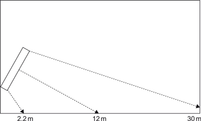
Figure 7.30 A simple speaker mounted at ear height.

There is a huge SPL variation from front to back—22.7 dB! People in the front row are being deafened (one of the authors has seen people close to the speakers wince in a York church installation), while people in the rear row are straining to hear anything.
Unfortunately this is not an unusual situation. Furthermore, the critical distance for this speaker is 2.63 m! So the %Alcons for this space will be 15.5%. Note that adding more speakers does not make the problem any better. Instead it makes it worse, because the extra loudspeakers further reduce the critical distance. In fact in a typical multi-speaker installation it is possible to show that an unaided human voice can be more intelligible than the PA system, provided the speaker can project their voice sufficiently!
The problem is that the path length variation is too large (2.2–30 m) and this results in a very high SPL variation. The arrangement would also have a very poor direct to reverberant ratio over most of the audience and would be prone to feedback. Let us see if using a more directive speaker mounted higher up can do any better.
Example 7.2
A single constant directivity horn speaker 7.5 m above ear height.
Mounting the speaker higher up, as shown in Figure 7.31, reduces the path variations between the front and back row. By making the speaker directive we can ensure that more of the sound goes to the audience. However, we have to handle the low frequencies with a separate loudspeaker because of the frequency limitations of the constant directivity horn.
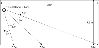
Figure 7.31 A single 40° × 60° constant directivity horn speaker mounted 7.5m above ear height.
Table 7.5 shows the results of doing this. Because of the lower variation in path length the path loss variation is lower: only 12 dB. However, the directivity of the loudspeaker both helps and hinders the total SPL at the listener. For the front row it overcompensates for the shorter path length and provides a slightly lower SPL there; unfortunately for the back row it adds to the path loss resulting in a lower SPL. The peak SPL variation is therefore 15.1 dB, which is better than the non-directive loudspeaker’s case, but still unacceptable.
Table 7.5 Calculated SPL for a single 40° × 60° constant directivity horn speaker

Although better, the directivity of one speaker is not precise enough to obtain an even distribution. What we need is more control over the directivity. Ideally we want an “on-axis” performance further down the audience. However, if we use a more directive horn then the front will suffer. So let’s see if by combining two horns to make a “central cluster” we can do better.
Example 7.3
Two constant directivity horn speakers 7.5 m above ear height.
We need to cover 60 degrees of angle using two constant directivity horns. This can be achieved by using a 60° × 40° combined with 40° × 20° horn, as shown in Figure 7.32; the horns are aligned so that the –6 dB points of the two horns are at the same angle. Because the signals are adding coherently these –6 dB points can become equivalent to an on-axis level. Therefore the combine horn has three “on-axis” points on the audience: one at 5.4 m, due to the 60° × 40° horn; one at 16.8 m due to the 40° × 20° horn; and finally one at 11.1 m due to the two horns combined. Note that we still have only one source of sound in the room despite using two speakers. This is because they both radiate sound energy from a single point.

Figure 7.32 A 60° × 40° horn combined with 40° X 20° horn at 7.5m above ear height.
Table 7.6 shows the results of doing this. Note that the 40° × 20° horn has a higher sensitivity, because it is concentrating the sound into a smaller solid angle. Note that the level is now much more uniform—to about halfway down the audience the maximum variation is 4.5 dB, or ±2.25 dB. However, the rear row at 30 m is still 14.5 dB lower than the level at 5.4 m, and this is still too much variation. One might be able to do better by using three horn loudspeakers, but this is getting more complicated and expensive. The main problem seems to be that the levels in the audience covered by the 40° × 20° horn are lower than those in the area covered by the other horn. So, as a more economical solution, let’s try raising the power fed to the 40° × 20° horn to 2.5 W, which is a +4 dB increase in level.

7.5.8 More than One Loudspeaker and Delays
Sometimes it is necessary to use more than one loudspeaker, for example to “fill in” a shaded under-balcony area, or cover a very wide area. In these situations the speakers should be as directive as possible so as to cover only the area required. This will minimize the amount of extra energy that is fed into the reverberant field. Electronic delay of the signal will often be required in order to match the acoustic delay. When this is used it should be set at about 15 ms greater than the acoustic delay. This has two advantages:
Two constant directivity horn speakers 7.5 m above ear height with more power to the horn covering the back.
Table 7.7 shows the results of doing this. Now the sound is more even within ±0.15 dB from 5 m to 19 m in the audience. It drops at the front and the back, and the maximum variation is 10.8 dB. In practice the front row is likely to receive additional sound from the stage, thus boosting its level. In general it is not a good idea to try to make the rear row the same level because this means the rear wall must be on-axis to a loudspeaker, which means half that speaker’s energy is splashing off the back wall and contributing to either the reverberant field or causing interference effects at the back of the venue. The calculated %Alcons for this design is 11%, which is on the boundary between acceptable and very good intelligibility.
Table 7.7 Calculated SPL for 1 W to the 60° × 40° horn 2.5 W to the 40° × 20° horn

We should also consider the lateral coverage. In the final arrangement the horn covering the front of the audience covers a wider angular width. This matches the trapezoidal audience shape seen by a high central cluster.
- Firstly, it allows the near speaker to be louder than the further one whilst giving the illusion that the sound is still coming from the further source via the Haas effect, as discussed in Chapter 2.
- Secondly, any combing effects due to the combination of the near and far signal are of a close enough frequency spacing (67 Hz) to be averaged by the ear’s critical bands and so not affect the intelligibility.
7.5.9 Objective Methods for Measuring Speech Quality
%Alcons is a subjective/empirical formula that can be used as a means of estimating the speech intelligibility from architectural data. However, for specifying systems it is better to have an objective measure that can be assessed by some form of acoustic instrumentation. Objective methods for measuring speech quality make use of either an auditory model or a measure that is based on a measure that is sensitive to speech spectral variations.
The articulation index (AI), now called the speech intelligibility index (SII) (Pavlovic, 1987), objectively measures “articulation” in individual critical bands, which is defined as that fraction of the original speech energy perceivable (i.e., between the threshold of hearing and the threshold of pain, and above the background noise). The AI can be measured by averaging the signal-to-noise ratio across all the bands. The validity of AI depends on the noise being non-signal dependent, which may not be the case with some processing. Also used are various measurements based on comparing the smoothed spectrum of the processed version with that of the original.
Another objective measure is the speech transmission index (STI) (IEC, 2003) (Houtgast and Steeneken, 1985), which uses a modulation transfer function approach to measure the effect of a given situation on speech intelligibility. It works for most forms of speech degradation and shows good correlation with subjective tests (Steeneken and Houtgast, 1994). It also has the advantage of being relatively easy to calculate, and so can be used in simulations to predict likely improvements in performance.
The criteria for STI and intelligibility are:
- 0.0 < STI < 0.4 intelligibility is poor
- 0.4 < STI < 0.6 intelligibility is fair
- 0.6 < STI < 0.8 intelligibility is good
- 0.8 < STI < 1.0 intelligibility is excellent.
It can also be measured, and the simpler STIpa and RaSTI methods that it replaces, are available as simple handheld instruments. For more details about public address system design see Ahnert and Steffen (1999).
7.6 Noise-Reducing Headphones
One important feature relevant to obtaining good quality audio listening is the relative levels of the wanted sound and unwanted sound such as local background acoustic noise. In environments such as aircraft cabins where the ambient acoustic noise level is high, it is not easy to obtain good quality audio. This is particularly the case with the headphones provided to economy class travelers, which are generally of a low quality that distorts the sound when the volume is turned up sufficiently high to hear the music or film soundtrack. There is also the danger that the overall sound level being presented (wanted signal plus the unwanted background noise) could even cause noise-induced hearing loss (see Section 2.5) depending on the volume of the wanted signal that is set.
One way of reducing the overall sound level being presented in such situations is to reduce the level of the unwanted acoustic background noise being experienced. This has the added advantage of perhaps improving the sound quality of the wanted sound because it can then be presented at a lower level, thereby possibly avoiding any distortion issues due to a high signal presentation level.
There are two common methods that are used for acoustic background noise reduction:
active noise cancellation
passive noise cancellation.
Active noise cancellation is based on the fact that if a waveform is added to an equal and opposite (antiphase) version of itself, cancellation results Figure 1.13). Active noise cancelation is designed into headphones which have a microphone on the outside of each earpiece to pick up the local acoustic background noise on each side of the head. This is essentially the acoustic noise that is reaching each ear. This microphone signal is phase reversed and added at the appropriate level to cancel the background noise. The wanted signal is also added in and the result is that the background noise is significantly reduced in level, and the overall volume of the wanted signal can be reduced to a more comfortable listening level.
Passive noise cancellation can be achieved with in-ear earphones that seal well in the ear canal. The principle here is to block the ear canal to reduce the level of acoustic background noise that enters the ear canal using the same technique used for in-ear ear defenders. Usually there are a number (two or three) of soft rubber flanges which form a seal with the border of the ear canal to attenuate the level of acoustic background noise that can enter the ear. The wanted sound is played via the earphones which are mounted in the body of the earphones, and the level of the wanted sound can be reduced as with active noise cancelation. Once again this allows a more comfortable overall acoustic level to be achieved and lessens the likelihood of sound distortion.
Both active and passive noise cancelation systems can work very effectively and many people (including both authors!) tend to prefer the passive type because only the wanted sound is being presented to the ear and the sound itself is not being modified in any way.
In the active case, the wanted signal is having noise added to it – not something one really wants to be doing if one can avoid it. If the phase shift is not absolutely correct, complete noise cancelation will not occur, with the result that the wanted signal is then being further contaminated. Furthermore, because of the phase shift requirement, higher frequencies are not attenuated as effectively—something the passive types do very well.
However, both kinds can sound very good in practice and whilst the sound is being modified in the active version, this needn’t modify or distort the wanted sound. The passive types are somewhat intrusive as their presence in the ear canal is felt physically since the seal has to be complete to enable them to function well. One advantage of a good seal with the ear canal is that transmission of the low-frequencies components is significantly improved.
7.7 “Mosquito” Units and “Teen Buzz” Ring Tones
Sound is being used to deter young people from congregating in particular areas via devices termed “mosquito units” or “teen deterrents.” These devices play sounds at relatively high levels that can only be heard by young people, thereby making it acoustically unpleasant for them to remain in a particular area. They can be placed outside shops, restaurants and other public places to discourage young people from hanging around there. The devices exploit the natural change in hearing response that occurs with age known as “presbycusis” (see Section 2.3) which causes a significant reduction in the ear’s ability to hear high frequencies (see Figure 2.11). The mosquito was invented by Howard Stapleton in 2005 and it was first marketed in 2006.
The nominal range of human hearing is usually quoted as being from 20 Hz to 20 kHz, but during a person’s twenties the upper frequency region reduces greatly in the range above about 16 kHz. The mosquito unit exploits this by emitting a sound between 16 and 19 kHz, which can only be heard by those less than 20–25 years of age. The usual range over which the mosquito operates as a deterrent is around 15–25 m. The UK National Physical Laboratory (NPL) conducted a test of the Mosquito (Ref E05110518, December 2005) in which they reported that the device presented:
- a mean f0 of 16.8 kHz;
- a maximum f0 of 18.6 kHz;
- an A-weighted sound pressure level of 76 dBA at 3 m;
- no hearing hazard under the UK Control of Noise at Work Regulations (April, 2006).
These units have proved themselves to be successful deterrents, saving considerable police time and effort in moving on gatherings of young people, and they are now used quite widely in public spaces. The unit will work in the presence of other sounds such as music, which typically contains no high-level energy at these high frequencies. Young people report these high-level high-frequency sounds to be very annoying, unpleasant and irritating.
However, young people now benefit from this basic idea because it has now been used to provide mobile ring tones, sometimes known as “teen buzz,” that cannot be heard by older people. The original teen buzz was created by recording the output from a mosquito device, but nowadays there are plenty of synthesized downloadable teen buzz ringtones available on-line. In general, these ring tones are not audible to adults over 25 years of age, but this does depend on the overall amplitude of the sound and the rate of presbycusis change for given individuals.
An example mosquito tone is provided on the accompanying CD to demonstrate what it sounds like; the track has four pure tones rising in octaves to the mosquito average frequency of 16.8 kHz as follows: 2.1 kHz, 4.2 kHz, 8.4 kHz and 16.8 kHz. Bear in mind when listening to this track that most youngsters will find the 16.8 kHz tone unpleasant; be cautious with the listening level.
7.8 Audio Coding Systems
Many of the advances in the distribution of audio material via film, DVD, television and the Internet, and even on DVD-Audio or Super Audio CD (SA-CD) have been made possible because of developments in audio coding systems. Audio coding systems are methods that reduce the overall data rate of the audio signal so that it may be transmitted via a limited data rate channel, such as the Internet, or stored in a data limited storage medium, like a DVD. In all cases the ability to reduce the data rate is essential for the system. There are two types of audio coding system:
- Lossless audio coding systems: In these systems the data rate, or data quantity, is reduced but in such a way that no information is lost. That is, after coding and subsequent decoding, the signal that comes out is identical to the signal that went in. This is like audio computer data file “zip” compression. Examples of such systems are: Shorten, an early lossless format; MPEG4 ALS, FLAC, Apple Lossless, examples of newer ones; and Direct Stream Transfer (DST) and Meridian Lossless Packing which are proprietary methods that are used in the SA-CD and DVD audio formats respectively. Lossless methods typically achieve a compression ratio of around 2 to 1. That is, the data size after compression is typically half the size of the input. The actual amount of compression achieved is dependent on the nature of the input audio signal itself (i.e., what kind of music it is or if it is speech) and can vary from about 1.5 to 1 to 3 to 1.
- Lossy audio coding systems: These systems make use of similar techniques to that of lossless coding but, in addition, reduce the data further by quantizing the signal to minimize the number of bits per sample. In order to achieve this with the minimum of perceived distortion, some form of psychoacoustic model is applied to control the amount of quantization that a particular part of the signal suffers. Because this type of coding removes, or loses, information from the audio signal it is known as a “lossy coding system.” Unlike the lossless systems these coders do not preserve the input signal; the output signal is not identical to the original input. The output signal is thus distorted but hopefully in a way that does not disturb and is inaudible to the listener. Examples of such systems are MPEG 1, MPEG 2, mp3, and MPEG 4, which are used on the Internet, in broadcasting and for DVDs. In the film world DTS, Sony-SDDS and Dolby AC3 are used to fit multiple channels onto standard film stock. The advantage of lossy coding is that it can compress the signal much more than a lossless system. For example, to achieve the 128 k bit data rate stereo audio that is used for mp3 coding of material on many music download sites, the audio signal has to be compressed by a factor of 11.025! This is considerably more than can be achieved by lossless compression.
So how do these systems work? What aspects of the audio signal allow one to losslessly compress the signal, and how can one effectively further reduce the data rate by doing psychoacoustic quantization?
7.8.1 The Archetypical Audio Coder
Figure 7.33 shows the three archetypical stages in an audio coder. All modern audio coders perform these operations. The decoder essentially operates in reverse. The three stages are:

Figure 7.33 Block diagram of an archetypical audio coder.
A signal redundancy removal stage which removes any inter-sample correlations in the signal. In order to do this, the coder may have to send additional side information to the receive end. This stage does not remove any information from the signal, it merely makes it more efficient and can therefore be considered to be lossless.
A psychoacoustic quantization stage which allocates bits to the various components in the audio signal in a manner that has the minimum subjective distortion. Again, in order to do this it has to send additional side information to the decoder, such as the number of bits allocated to each signal component. This is the only stage that removes information from the signal and is therefore the only lossy stage in the whole process. It is this stage that makes the difference between a lossy and a lossless audio coding system. Note that although the decoder stage works in reverse to provide real audio levels at the levels quantized by the coder, it cannot restore the information that has been thrown away by the encoding quantizer.
An entropy coding stage which tries to use the most efficient bit arrangement to transmit both the signal information and the side information to the decode end. This stage also does not remove any information from the signal and can also be considered to be lossless.
The purpose of these three stages is to maximize the amount of audio information transmitted to the receive end. So in order to understand how these stages work we need to understand what we mean by information and how it is related to the audio signal. Then we can unpack the function of the three stages in more detail.
7.8.2 What Exactly is Information?
What characteristics of a signal or data stream indicate information? For example, you are currently reading text in this book; what is it about the text that is carrying information? The answer is that, as you read it, you are seeing new combinations of words that are telling you something you didn’t know before. Another way of looking at it is there is an element of novelty or surprise in the text. On the other hand, if, during a web chat, you got a message that said “hhhhhhhhhhhhhhhhhhhhhhhh …” it would be carrying no information, other than the possibility that the other person has fallen asleep on the keyboard! So the more surprising a thing is the more information it carries. That is, the less probable something is the more information it carries. So:
![]()
How does this relate to an audio signal? Well, consider a sine wave; it sounds pretty boring to listen to because it is very predictable. On the other hand, a piece of music that is jumping around, or an instrument whose texture is continuously changing, is much more interesting to listen to because it’s more unpredictable or surprising. If we looked at the spectrum of a sine wave we would find that all the energy is concentrated at one frequency whereas for the more interesting music signal it’s spread over lots of frequencies. In fact the audio signal that carries the most information is either random noise, or a single spike that happens at a time you don’t or can’t predict. Interestingly, in both these cases the spectrum of the signal contains an equal amount of energy at all frequencies. Again, just like text, the more surprising a signal is the more information it carries.
So to maximize the information carried by our coded audio signal we first need to maximize the surprise value of the audio signal. This is done by the signal redundancy removal stage.
7.8.3 The Signal Redundancy Removal Stage
In Chapter 4 we saw that all musical instruments, including the human voice, could be modeled as a sound source followed by sound modifiers, which apply a filtering function. In the limit the source may be regular spaced impulses, for pitched instruments, a single pulse for percussion instruments, random noise for fricatives, or a combination of them all. A filter that combines the effect of the source with the acoustic effect of the instrument and output to shape the final sound then follows this. The effect of this filtering is to add correlation to the audio signal. Correlation implies that information from previous samples is carried over to the current sample, as shown in Figure 7.34. The basic principle behind redundancy removal is that at a given time instant the audio signal will consist of two elements (as shown in Figure 7.34).

Figure 7.34 Information in a sample at a given time due to previous samples.
- Information about the previous signals that have passed through the filter. In principle the contribution of this to the overall signal can be calculated from knowledge of the signal that has already passed through the filter. That is, this contribution is predictable; this is shown by the different hatchings in the sample at time “t” in Figure 7.34 that correspond to the similarly hatched earlier samples.
- Information that is purely due to the excitation of the filter by the source. The contribution of this to the overall signal cannot be calculated from knowledge of the signal that has already passed through the filter and hence this contribution is not predictable, and is shown in black on Figure 7.34.
To maximize the information content of the signal we should aim to remove the predictable parts, because they can be recalculated at the receive end, and only encode the unpredictable part because this represents the new information.
This is what the correlation removal stage does. There are two different ways of doing this:
- Time domain prediction: This is the method used by most lossless encoding schemes, which calculates an inverse filter to one that has filtered the unpredictable parts of the signal. It is possible, using the method of linear prediction, to calculate the necessary inverse filter from the input data. This filter is then used to remove the correlated components from the input signal, prior to coding the signal. At the decoder the original signal is recovered by feeding the decoded signal into the complementary filter, which then puts the correlations back into the signal. To do this the coder must send additional side information that specifies the necessary filter coefficients so that the decoder restores the correlation correctly. In addition, because the correlations within the signal vary with time, due to different notes and instruments, it is necessary to recalculate the required filter coefficients and resend them periodically. Typically this happens at about 50 to 100 times a second. This type of system is known as a “forward adaptive predictor” because it explicitly sends the necessary reconstruction information forward to the decoder. There is an alternative known as a “backward adaptive predictor” that sends the necessary side information implicitly in the data stream, but it is seldom used.
- Frequency domain processing: This is the method used by most of the lossy audio coding schemes, which splits the audio spectrum into many small bands. In principle the smaller the better, but there is a limit to how far one can do this because smaller bands have a longer time response, as discussed in Chapter 1. It practice, due to the limitations imposed by temporal masking (see Chapter 5) the time extent of the signal is limited to 8–25 ms, which implies a minimum bandwidth of 125–40 Hz. This technique removes correlation from the signal because although each band will have a different amplitude level, which implies correlation. These can be normalized by applying an appropriate scale factor to each band, which effectively removes correlation, and the narrower the bands are the more effective this removal can be. It also allows the coder to flag bands that contain no energy at all and therefore no information needs to be transmitted. These scale factors and unused band information need to be transmitted to the decoder and therefore represent additional side information to be encoded and transmitted to the decoder. The signal within the bands is also less correlated because, as the band gets narrower in frequency range, the spectrum within the band is more likely to be uniform, and thus approaches the desired white noise spectrum with zero correlation between samples. A further advantage of frequency domain processing is that it converts the audio signal into a form that makes it easy for psychoacoustic quantization to be efficiently applied.
The use of either a time or frequency domain method is possible, and their relative strengths and weaknesses are primarily determined by the application. For example, the frequency domain approach fits well with psycho-acoustic quantization algorithms – hence its choice for lossy coding systems.
However, all signal redundancy removal schemes have to tread an uneasy balance between increasing their effectiveness, which requires more side information, and having sufficient resources to effectively encode the actual audio signal information.
7.8.4 The Entropy Coding Stage
Although the entropy stage is the final stage in the coder, it is appropriate to consider it now because in conjunction with the redundancy removal stage it forms the structure of a lossless encoder system. Entropy encoding works by maximizing the information carried by the bit patterns that represent the audio signal and the side information. In order to understand how it works we need to understand a little bit about how we measure information and how entropy relates to information.
7.8.5 How do we Measure Information?
In order to measure the information content of a signal we need to know how likely it is to occur. However, we also want to be able to relate the information content to something real, such as the number of bits necessary to transmit that information. So how could we measure information content in such a way that it is related to the number of bits needed to transmit it?
Consider a 3-bit binary digit. It has eight possible bit patterns, or symbols, as shown in Table 7.8. Furthermore let’s assume that each possible symbol has the same one in eight probability of happening occurring (Psymbol = 0.125). If we use the following equation:
Table 7.8 Symbols associated with a 3-bit binary code
| Binary code | Symbol |
000 | 0 |
001 | 1 |
010 | 2 |
011 | 3 |
100 | 4 |
101 | 5 |
110 | 6 |
111 | 7 |

where Isymbol = | the self-information of the symbol (in bits) |
Psymbol = | the probability of that symbol occurring |
log2 = | the logarithm base 2, because we are dealing in bits |
One can calculate log2(x) simply as follows:
![]()
Where: log10(x) Is the logarithm base 10, the standard log key on most calculators
For any of the eight symbols shown in Table 7.8, the self-information is 3 bits because they all have the same probability. However, if the probability of a particular symbol was one, i.e., it was like our repeating “h” discussed earlier, the self-information would be zero. On the other hand, if the probability of one of the symbols was lower than one-eighth, for example, one-hundredth or (0.01), then that symbol’s self-information would be log2(1/0.01), which would equal 6.64 bits, which would mean that symbol was carrying more information than the other symbols.
Because the total probability of all the symbols must add up to one, if one symbol has a very low probability then the probability of the other symbols must be slightly greater to compensate. In the case of one symbol having a probability of one-hundredth, the other symbols taken all together will have to have a probability of Psymbol = (99/(7 × 100)) = 0.141. This gives a self-information for all the other symbols of 2.83 bits per symbol. So in this case one symbol is worth more than 3 bits of information, but the other symbols are worth less than 3 bits of information. So one of the symbols is using the bits more efficiently than the other seven symbols.
To unravel this we must look at more than the self-information carried by each symbol. Instead we must look at the total information carried by all the symbols used in the data stream.
7.8.6 How do we Measure the Total Information?
In the previous section we had the case of one symbol in the whole set of possibilities being very small and as a consequence the other seven symbols had to have a higher probability, because the probability of all symbols being used has to be one. As an extreme case consider our person asleep on the keyboard who is sending the same symbol all the time. In this case the probability of the symbol being sent is one, and all other symbols have zero probability of being sent. The total information being sent by this source is zero bits. How can this be? Surely, if the probability is zero, then the self-information of these symbols is infinite? In theory this might be true but, as these symbols are never sent, the total information is zero.
So in order to find out the total information of the source we need to incorporate not only the self-information of each symbol but also their probability of being sent. This gives the proportion of information that symbol actually carries as part of the whole data set. To do this we simply multiply the self-information of the symbol by the probability of that symbol actually occurring. This gives the amount of information that symbol carries in proportion to the other symbols in the data source.

This is also known as the “entropy” because the equation is analogous to one used to calculate entropy in physics. In general we are interested in the total information content, or entropy of the data source, because this gives us the minimum number of bits required to encode it. This is given by:

Equation 7.11 shows that the way to calculate the entropy of a data source is to add up all the individual symbol entropies of that source.
Table 7.9 shows the calculated entropy for four different data sources—the first three correspond to the examples that have been discussed already and the fourth represents the output of a 5-level audio signal. Notice that, except for the case of all symbols having equal probability, all the other sources have a total source information, or entropy, of less than 3 bits. This is always true: the most efficient information source is one that uses all its possible symbols with equal probabilities. If we encoded the sources shown in Table 7.9 using a 3-bit binary code, then we would be wasting bits. In principle we could code the audio signal using only 1.7 bits, but how?
Table 7.9 Source entropies for a 3-bit binary code with different symbol probabilities

This is the idea behind entropy coding; what we need is a transmitted code that relates more closely to the entropy of each symbol.
7.8.7 Entropy Coding
In order to implement entropy coding we have to more closely match the number of bits we use for each symbol to the amount of information it carries. Furthermore, each codeword associated with the symbol must have an integer number of bits. The net result of this is that instead of using a fixed number of bits for each symbol we need to use a number of bits that is related to the information carried by that symbol. For example, we know that in a real audio signal the signal spends much more time at low amplitudes than high amplitudes, so low amplitudes carry less information and should be encoded with fewer bits than high signal levels. This way fewer bits would be used, on average, to transmit the information. But how do we generate codes that have this desirable property? One simple way of doing it is by using a technique called Huffman coding, which is best illustrated by an example.
Consider the 5-level audio signal shown in column 6 of Table 7.9. At the moment we are using 3 bits of information to transmit an information source that only has 1.7 bits of information. How can we assign code words to the symbols such that the average data rate is closer to 1.7 bits? Firstly, we can recognize that three of the symbols are not used and hence can be ignored.
A Huffman code is generated by starting with the least probable symbol. The list of symbols is first sorted into a list of decreasing probability, as shown in Table 7.10. Then, working up from the lowest probability symbol, a code is constructed by combining the probabilities together to form different levels that correspond to bits in the code. These bits are then used to select either a code word or the next level down, except for the longest/lowest level, corresponding to the two lowest probability symbols in which the bit is used to select between a one and a zero.
Table 7.10 Forming a Huffman code for a 5-level audio signal

By allocating a bit for each level, a variable length code is built up where a leading zero represents the beginning of a new code word, up to the maximum length of the codewords. This property makes the code comma free, which means it needs no additional bits to separate the variable code words from each other, thus maximizing the efficiency. A code word of length one is assigned to the most probable symbol and longer length code words are optimally assigned to the lower probability symbols.
One can calculate the average bits per symbol, after coding, by simply using the actual bits it uses and multiplying that by its probability of occurring. This gives that symbol’s average bit rate. Then, by adding up the average bit rate for all the symbols, you get the total average bit rate:
![]()
In our example the rate calculation becomes:
BitRateactual = 0.6 × 1 + 0.15 × 2 + 0.15 × 3 + 0.05 × 4 + 0.05 × 4
Which gives: BitRateactual = 1.75 bits symbol–1
Huffman coding is optimal in that it gets the code rate within one bit of the source entropy. However, because bits only come in integer multiples the efficiency for small symbol sets is quite low. In MPEG_1 layer 3 coders, some symbols are Huffman coded as pairs to allow a greater coding efficiency. However, there is a practical limit to the size of a Huffman code because the computation and the tables blow up exponentially in size and so become unfeasible. A more subtle limitation is that, for large symbol sets, it becomes very difficult to gather enough symbol statistics data with sufficient accuracy to generate a Huffman code.
In order to have longer symbol lengths, which allow greater coding efficiencies, other approaches are used. Golomb Rice Codes use a predetermined statistical distribution to remove the need for tables, thus allowing longer code words; they are used in some lossless encoding schemes. Another approach is Arithmetic Coding, which does not need predetermined distributions but, by using the statistics of the symbols occurrence, can encode very long symbols and so approach the source entropy much more closely. For details about these and other entropy coding methods see Salomon (2007).
7.8.8 The Psychoacoustic Quantization Stage
This is the stage that makes the difference between a lossless and a lossy coder. Again the actual signal processing can be carried out in either the time domain or the frequency domain. In both cases the process of adaptive quantization and noise shaping is used.
7.8.9 Quantization and Adaptive Quantization
Quantization is the process of taking an audio, or video, signal and converting it to a discrete set of levels. The input to this process may be from a continuous audio signal, like the one you get from a microphone, or may be from an already quantized signal, for example, the signal from a compact disc. An important parameter is the number of levels in the quantizer. This is due to the fact that the act of quantization is lossy because it throws away information. If the input signal is not exactly the same as the desired output then there will be an error between the input and the output, as shown in Figure 7.35.

Figure 7.35 The input, output and error of a quantizer.
Although the quantizer will pick the output level that causes minimum error, there will on average always be some error. This error adds noise and distortion to the signal and is often referred to as quantization noise. Ideally this noise should be random and often dither is added to ensure this. The effect of the error is to reduce the signal to noise ratio of the audio signal. If a binary word of Nbits bits is used to encode the audio signal, then the maximum signal to noise ratio is given by:
![]()
For a 16-bit word (the CD standard), this gives a maximum signal to noise ratio of 96 dB. If you compare this signal to noise ratio with the idealized masked thresholds in Figure 5.9 in Chapter 5, you will see that the quantization noise will be masked over most of the audio band for loud signals. Although quantizers very often have a number of levels, that are powers of 2, such as 16, 256 or 65 536, because this makes best use of a binary word, there is no reason that other numbers of levels cannot be used, especially if entropy coding is going to be employed. In this case the maximum signal to noise ratio for an N level quantizer will be given by:
![]()
In either case, the quantization error is uniform over the frequency range in the ideal case.
These maximum signal to noise calculations are assuming that both the signal and noise have a signal probability distribution that is uniform; that is, all signal levels within the range of the quantizer are equally possible. If one assumes a sine wave input at maximum level then the maximum signal to noise ratio is improved, by + 1.76 dB, because a sine wave spends more time at higher levels. However, in general we do not listen to either sine waves or uniform random noise. We listen to signals that spend more time at low signal levels and this means that often the signal to noise ratio is worse than predicted by these equations.
Real signals often spend most of their time at low signal levels, but one has to design the quantizer to handle the maximum signal level, even if it isn’t used very often. This means that more bits are used than is strictly necessary most of the time. One way of reducing the number of bits needed to quantize an audio signal is to make the quantizer adapt to the level of the signal because loud signals mask weaker signals, as discussed in Chapter 5. This type of quantizer is known as an “adaptive quantizer,” and can save some bits. There are two main types of adaptive quantizer:
Backward adaptive quantizers (Jayant, 1973): These make use of the adapted output bits to drive the adaptation and so require no additional bits to be sent to the receive end. However, they are sensitive to errors and are not guaranteed to be overload-free. Although there are ways of mitigating these problems they are not often used in lossy compression systems.
Forward adaptive quantizers: Look at a block of the input signal and then set a scale factor that makes maximum use of the quantizer. This type of adaptive quantizer is guaranteed to be free from overload and is more robust to errors. However, it needs some side information—the scale factor—to be sent to the receive end, which clearly robs bits from the quantized signal samples. Therefore there is an uncomfortable balance that must be struck between the amount of side information and the number of levels in the adaptive quantizer. In particular, if the block is made longer then less scale values have to be sent to the receiver. But if the block is too long then the quantization noise may become unmasked, due to non-simultaneous masking. So the block size is set typically within the range 8–25 ms to avoid this happening. There is also an issue about the scale precision. The minimum scale precision is 6 dB which allows for a very simple implementation, but there is a possibility that only just over half the quantizer’s range is used because if the input has a sample that is just over half the quantizer’s range then the scale would set to that case, as the next lower scale value would result in an overload. Increasing precision of the scale factor would allow a greater proportion of the quantizer to be used on average, but would require the scale value to have a longer word length to handle the increased precision. This increases the amount of side information that must be sent to the receiver. MPEG uses finer scale factors of 1.5 dB to 2 dB.
Adaptive quantizers attempt to make the input signal statistics match the ideal uniform distribution for maximum signal to noise. However, even with fine-scale steps this is rarely achieved and there is still a tendency for the small signal levels to be more probable. Furthermore, the higher levels may have a better signal to noise ratio than is strictly necessary for masking.
One solution to this is to use non-uniform quantization, sometimes called non-linear quantization, in which the levels are not equally spaced. By having the less probable higher levels further apart, the increased quantization error that results is more likely to be masked by the signal, and, because it’s less probable, the average signal to noise level does not increase. In fact, for a given number of levels the average signal to noise reduces because the more likely levels are closer together and thus generate less quantization noise. MPEG-1 layer 3 uses a non-uniform quantizer to quantize the filtered signal samples.
However, even if an adaptive quantizer is used, then, because of the uniform spectrum of the quantization noise, the overall noise becomes unmasked if the signal to noise ratio falls below about 60 dB. This corresponds to 10 bits of quantizer precision. In order to do better we need to arrange for the noise to be shaped so that it is less perceptible.
7.8.10 Psychoacoustic Noise Shaping
As discussed in Chapter 2, our threshold of hearing is not constant with frequency, as shown in Figure 2.14. We are much more sensitive to sounds around 4 kHz than at the extremes of the frequency range. Therefore a uniform quantization spectrum may be more inaudible at low and high frequencies and yet still be heard if it is above the threshold of hearing in the most sensitive part of our hearing range. Ideally we need to have more noise where we are less sensitive to it and less noise where we are more sensitive. This is possible via a technique known as “noise shaping.”
Figure 7.36 shows the block diagram of a noise-shaping quantizer. In it the quantization error is extracted, fed back via a noise-shaping filter and subtracted from the input. The effect of this can be analyzed as follows, assuming that the output of a quantizer can be considered to be the sum of the input signal and the quantization error.

Figure 7.36 Block diagram of a noise-shaping quantizer.
![]()
Which gives:
![]()
Equation 7.15 shows that the quantizer’s error is shaped by the filter function (1 – N(z)). It is possible to design this filter to reduce the noise within the most sensitive bit of our hearing range. This technique is used to improve the quality of sounds on a CD. An example is Sony Super Bit Mapping (Akune et al., 1992), which uses psychoacoustic noise shaping to give an effective signal to noise ratio of 120 dB (20 bits) in our most sensitive frequency range.
7.8.11 Psychoacoustic Quantization
Although noise shaping provides a means of psychoacoustically shaping the quantization noise, it is difficult to achieve very low bit rates using it. In particular one needs to be able to avoid transmitting information in frequency regions that either contain no signal, or are masked by other signal components. To do this easily one must work in the frequency domain.
Figure 7.37 shows the block diagram of a lossy audio coder. Ideally the time to frequency mapping splits the signal up into bands that are equal to, or smaller than, the width of our critical bands. Unfortunately for some audio coders this is not true at the lower frequencies.

The psychoacoustic quantization block is now replaced by a bit allocation and quantization block, which is driven by a psychoacoustic model that allocates the number of quantization levels for each frequency band, including zero for no bits allocated. Psychoacoustic models can be quite complicated and are continuously evolving. This is because most lossy audio coding systems define how the receiver interprets the bit stream to form the audio output, but leave how those bits are allocated the bit allocation to the encoder. This is clever because it allows the encoder to improve, as technology and knowledge get better, without having to alter the decoder standard. This is an important consideration for any audio delivery format.
However, regardless of the psychoacoustic bit allocation algorithm, they all effectively convert the linear frequency scale of the discrete Fourier transform into a perceptually based frequency scale similar to the ERB scale shown in Figure 5.10. Most use the Bark scale, which is similar but is based on the earlier work of Zwicker. Both scales are quasi-logarithmic and convert simultaneous masking thresholds into approximately straight lines.
Using some form of simultaneous masking model masking curves, which are different for tonal and non-tonal sounds, a signal to masking ratio (SMR) is calculated and the bits allocated such that components that need a high SMR are given more bits than those that have a lower SMR. For components that have a negative SMR no bits are allocated because these components are masked and therefore need not be transmitted. The amount of bits that can be allocated depends on the desired bit rate. Also, the process interacts with itself so this process usually is inside some form of optimization loop that minimizes the total perceptual error. For more information the book by Marina Bosi (Bosi and Goldberg, 2003), one of the developers of current lossy coding systems, provides a wealth of information.
7.9 Summary
This chapter has looked at a variety of applications that combine both acoustic and psychoacoustic knowledge to achieve a specific audio objective. The need to combine both these aspects of this knowledge to achieve useful results, and the diversity of applications are what make this subject so exciting! As we write, acoustics is being applied to many more areas that affect our everyday life directly, for example the noise caused by wind farms, acoustic screening between individual working spaces in open office areas, and the design of urban public spaces that not only look nice but also sound good. Our hearing is one of our most precious senses, and it good to see that, as we become more technologically sophisticated, we are coming to realize that, for our human existence, sound really matters!
References
Ahnert, W, Steffen, F., 1999. Sound Reinforcement Engineering: Fundamentals and Practice. Spon, London.
Bech, S., Zacharov, N., 2006. Perceptual Audio Evaluation – Theory, Method and Application. Wiley.
Bosi, M., Goldberg, R.E., 2003. Introduction to Digital Audio Coding and Standards, second edn. Springer, NY and London.
D’Antonio, P., Konnert, J.H., 1984. The RFZ/RPG approach to control room monitoring. Audio Engineering Society 76th Convention, October, New York, USA, preprint #2157.
Davies, D., Davies, C., 1980. The LEDE concept for the control of acoustic and psychoacoustic parameters in recording control rooms. J. Audio Eng. Soc. 28 (3), 585–595 (November).
Houtgast, T., Steeneken, H.J.M., 1985. The MTF concept in room acoustics and its use for estimating speech intelligibility in auditoria. Journal of the Acoustical Society of America. 77, 1069–1077.
Howard, D.M., 1991. Speech: measurements. In: Payne, P.A. (Ed.), Concise Encyclopaedia of Biological and Biomedical Measurement Systems. Pergamon Press, Oxford, pp. 370–376.
IEC 60268-13:1998, BS 6840-13:1998 (2003). Sound system equipment. Listening tests on loudspeakers IEC standard n. 60268-16. Sound System Equipments – Objective rating of speech intelligibility by speech transmission index, July 2003.
IEC standard n. 60268-16. Sound System Equipments – Objective rating of speech intelligibility by speech transmission index, July 2003.
ISO/TR 4870:1991 Acoustics—The construction and calibration of speech intelligibility tests.
Jayant, N.S., 1973. Adaptive quantization with a one-word memory. Bell Systems Technical Journal. 52, 1119–1144 (September).
Newell, P., 2008. Recording Studio Design, second edn. Focal Press, Oxford.
Pavlovic, C.V, 1987. Derivation of primary parameters and procedures for use in speech intelligibility predictions. Journal of the Acoustical Society of America. 82, 413–422.
Peutz, 1971. Articulation loss of consonants as a criterion for speech transmission in a room. J. Audio Eng. Soc. 19 (11), 915–919; December.
Rodgers, C.A.P., 1981. Pinna transformations and sound reproduction. J. Audio Eng. Soc. 29 (4), 226–234 April.
Rumsey, F., 2001. Spatial Audio (Music Technology Series). Focal, Oxford.
Salomon, D., 2007. Data Compression: The Complete Reference, fourth edn. Springer, New York & London.
Toole, F. E., 1990. Loudspeakers and Rooms for Stereophonic Sound Reproduction. In: The Proceedings of the Audio Engineering Society 8th International Conference, The Sound of Audio, Washington, DC, 3–6 May, pp. 71–91.
Walker, R., 1993. A new approach to the design of control room acoustics for stereophony. Audio Engineering Society Convention, preprint #3543, 94.
Walker, R., 1998. A controlled-reflection listening room for multichannel sound. Audio Engineering Society Convention, preprint #4645, 104.
Further Reading
Akune, M., Heddle, R., Akagiri, K., 1992. Super bit mapping: psychoacoustically optimized digital recording. Audio Engineering Society Convention 93, preprint # 3371.
Angus, J.A.S., 1997. Controlling early reflections using diffusion, Audio Engineering Society 102nd Convention, 22-25 March, Munich, Germany, preprint #4405.
Angus, J.A.S., 2001. The effects of specular versus diffuse reflections on the frequency response at the listener. J. Audio Eng. Soc. 49 (3), 125–133 (March).
ANSI S3.5-1997, American National Standard Methods for Calculation of the Speech Intelligibility Index. American National Standards Institute, New York.
Holman, T., 1999. 5.1 Surround Sound. Focal Press, Boston.
Newell, P., 1995. Studio Monitoring Design. Focal Press, Oxford.
Newell, P., 2000. Project Studios: A More Professional Approach. Focal Press, Oxford.
Schroeder, M.R., 1975. Diffuse sound reflection by maximum-length sequences. J. Acoust. Soc. Am. 57 (January), 149–151.
Schroeder, M.R., 1984. Progress in architectural acoustics and artificial reverberation: concert hall acoustics and number theory. J. Audio Eng. Soc. 32 (4), 194–203 April.
Steeneken, H.J.M. and Houtgast, T., 1994. Subjective and objective speech intelligibility measures. Proceedings of the Institute of Acoustics, 16(4), 95–112.
Toole, F., 2008. Sound Reproduction: the Acoustics and Psychoacoustics of Loudspeakers and Rooms. Focal Press, Oxford.
Walker, R., 1996. Optimum dimension ratios for small rooms. Audio Engineering Society Convention, preprint #4191, 100.