
8.1 Introduction
8.2 Numerical Differentiation
8.3 Numerical Integration
8.4 Visual Solution: Code8
8.5 Summary
Numerical Exercises
Programming Challenges
The derivative of a function gives a clear indication of the rate of increase or decrease of the function with respect to its domain. The rate of increase or decrease of a function contributes to the overall understanding of a system that is governed by such parameters. In general, the derivatives of a function contribute to the modeling of a given problem, which describes the properties and dynamics of the elements in the problem. For example, in studying the electrostatic field properties of an area, the solution requires a graphing of the first and second derivatives of the points in the area. We will discuss some useful properties of the derivatives of a function for modeling in the next few chapters.
The analytical derivative of a function f (x) with respect to the variable x is denoted by f' (x) or
By default, a digital computer does not have the processing capability to produce the analytical derivative of a function. However, this analytical solution can still be produced through a software that stores a list of primitive functions and its derivatives in a numerical database. On the computer, the analytical solution to a derivative is a complex problem that requires several recursive calls to the functions in its numerical database. Symbolic computing is one area of study that addresses this problem, which involves the construction of a database of mathematical functions for generating the analytical solution to their derivatives.
The computer gives a good approximation to the derivatives of a function based on some finite points in the given domain. A numerical approximation to the derivative of as a function f (x) is a solution expressed as a number, rather than as a function of x. The domain of f (x) is first decomposed into its discrete form, x i for i = 1, 2, ..., m, and the derivatives are computed at these points based on their relative points.
An integral of a function does the opposite of derivative. Integral returns the differentiated function to its original value. A numerical approach for finding the integral of a function is needed in cases where the integral is difficult to compute.
In this chapter, we will discuss several numerical approaches to finding the derivatives and integral of a function. The approximated values returned from the methods are reasonably close to the exact values and are acceptable in most cases.
The starting point in finding a derivative is the nth-order Taylor series expansion of a discrete function y i = f (x i) given as follows:
Equation (8.1) gives the one-term forward expansion of y = f (x). In this equation, h = Δ x is the width of the x subintervals that are assumed to be uniform. The term yi+1 = f (x i+1) above is equivalent to y i+1 = f (x i+1) = f (xi + h).
Figure 8.1 shows the relative position of the discrete points of f (x) in the interval xi−2 ≤x ≤ xi+2. Taking only up to the second derivative term, this equation reduces to

Obviously, the one-term forward expansion in Taylor series involves x i +1 = x i + h. In a similar manner, we can define the two-term forward expansion by replacing h with 2h, or x i +2 = x i + 2h, to produce
It follows that the one-term backward expansion is obtained by replacing h with −h, or xi−1 = xi + (−h) = xi − h, to produce
Subsequently, the two-term backward expansions of y = f (x) involve xi−2 = xi + (−2h) = xi − 2h and are given by
The simplest rule for the first derivative is obtained by taking y'i as a subject in the first two terms of Equation (8.1). It produces the forward-difference rule for the first derivative,

The forward-difference rule for the second derivative is obtained by subtracting twice Equation (8.2c) from Equation (8.2d) and by simplifying the terms to produce
There is also the backward-difference rule for the first derivative, obtained by taking y'i as a subject in the first two terms of Equation (8.2c), to produce
Similarly, subtracting twice Equation (8.2c) from Equation (8.2d) gives the backward-difference rule for the second derivative:
As the names suggest, the forward-difference and backward-difference rules have the disadvantage in that they are bias toward the forward and backward points, respectively. A more balanced approach is the central-difference rules, which consider both forward and backward points. Subtracting Equation (8.2a) from (8.2c) and simplifying terms, we obtain the central-difference rule for the first derivative.
By adding Equations (8.2a) and (8.2c) and simplifying the terms, we obtain the central-difference rule for the second derivative.
Example 8.1. Given y = x sin x, find y' and y" at the points along 0 ≤x ≤ 2 whose subintervals have an equal width given by h = 0.3333 using the forward, backward, and central-difference methods.
Solution. In this problem, m = (2 − 0)/.3333 = 6. The analytical derivatives are given by y' = sin x + x cos x and y" = 2 cos x − x sin x. Table 8.1 plots the values of xi and yi for i = 0, 1, ..., 6. The analytical derivatives at these points are shown in the fourth and fifth columns of the table.
At i = 0, y'0 and y"0 can be evaluated using the forward-difference rules using Equation (8.3a) and (8.3b):
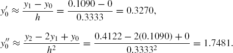
It is not possible to evaluate y'0 and y"0 using the backward and central-difference rules as both methods involve the terms y−1 and y−2, which do not exist. The results at other points are shown in Table 8.1. Through comparison with the analytical (exact) method, the central-difference method produces the closest approximations for the derivatives.
Table 8.1. The numerical results from Example 8.1
| Analytical Solutions | Forward-difference | Backward-difference | Central-difference | |||||||
|---|---|---|---|---|---|---|---|---|---|---|
i | xi | yi | y'i | y"i | y'i | y"i | y'i | y"i | y'i | y"i |
0 | 0 | 0 | 0 | 2 | 0.3270 | 1.7481 | void | void | void | void |
1 | 0.3333 | 0.1090 | 0.6421 | 1.7809 | 0.9097 | 1.1342 | 0.3270 | void | 0.6183 | 1.7481 |
2 | 0.6667 | 0.4122 | 1.1423 | 1.1594 | 1.2877 | 0.2277 | 0.9097 | 1.7481 | 1.0987 | 1.1342 |
3 | 1.000 | 0.8414 | 1.3818 | 0.2391 | 1.3636 | −0.8228 | 1.2877 | 1.1342 | 1.3257 | 0.2277 |
4 | 1.3333 | 1.2959 | 1.2856 | −0.8255 | 1.0894 | −1.8319 | 1.3636 | 0.2277 | 1.2265 | −0.8228 |
5 | 1.6667 | 1.6590 | 0.8358 | −1.8515 | 0.4788 | void | 1.0894 | −0.8228 | 0.7841 | −1.8319 |
6 | 2.000 | 1.8186 | 0.0770 | −2.6509 | void | void | 0.4788 | −1.8319 | void | void |
An integral of the form
The exact methods for evaluating definite integrals have been widely discussed in elementary calculus classes. Some popular methods involve techniques such as direct integration, substitutions, integration by parts, partial fractions, and substitutions with the use of trigonometric functions. However, not all definite integral problems can be solved using such methods. This may be the case when the function f (x) is too difficult to integrate, or in the case where f (x) is given in the form of a discrete data set. Furthermore, it may not be possible to implement the exact method on the computer as the computer does not have the analytical skill like a human does. Therefore, approximations using numerical methods may prove to be an alternative approach and practical for implementation here.
Numerical solutions for evaluating definite integrals are obtained using several methods. Some of the most fundamental methods include the trapezium, Simpson, Simpson's 3/8, and Gaussian quadrature methods. We discuss these methods in this section.
The trapezium method is a classic technique for approximating the definite integral of a function

In the trapezium method, the x interval in a ≤ x ≤ b is divided into m equal-width subintervals, each with width h. A straight line is connected from (xi, f (xi)) to (xi+1, f (xi+1)) in the subinterval [xi, xi+1], and this forms a trapezium with f (xi) and f (xi+1) as the parallel sides whose distance between them is h. The area under the curve in this subinterval is then approximated as the area of the trapezium, given as
With m subintervals,

Equation (8.6) gives the trapezium method for finding the definite integral of a function f (x) in the interval from x = a to x = b with m equal subintervals. The method is illustrated in Figure 8.3 using four equal subintervals. From the figure, it is clear that


Example 8.2. Find
Solution. In this problem, m = 9, x0 = 0, and xm = 3. The width of each subinterval is
i | 0 | 1 | 2 | 3 | 4 | 5 | 6 | 7 | 8 | 9 |
|---|---|---|---|---|---|---|---|---|---|---|
xi | 0 | 0.3333 | 0.6667 | 1.0000 | 1.3333 | 1.6667 | 2.0000 | 2.3333 | 2.6667 | 3.0000 |
yi | 0 | 0.1090 | 0.4122 | 0.8414 | 1.2959 | 1.6590 | 1.8186 | 1.6872 | 1.2194 | 0.4234 |
Therefore,
The trapezium method uses a straight line approximation on two successive f (x) values in the subintervals for evaluating
The accuracy of the trapezium method can be improved by replacing the straight line with a quadratic function. This idea makes sense as a quadratic curve lies closer to the real curve in the given function than a straight line. Since a quadratic function requires three points for interpolation, the method suggests pairs of two subintervals in the approximation. The approach is called the Simpson method.
As the Simpson method requires two subintervals in each pair, the total number of subintervals in the given interval must be an even number. Consider the subintervals [xi, xi+1] and [xi+1, xi+2], which involve the points, (xi, f (xi)), (xi+1, f (xi+1)), and (xi+2, f (xi+2)). Figure 8.4 shows this scenario with the dotted curve as the quadratic approximation to the real curve. This curve has an equation given by

where a0, a1, and a2 are the constants that are to be determined. The quadratic curve interpolates (xi, y i), (xi +1, yi+1) and (xi +2, yi+2). This produces a system of linear equations, given as

The above system is solved to produce the Simpson's formula, given by
Equation (8.7) can be extended into the case of m even subintervals for x = x0 to x = x m. The total area is found as a sum of m/2 subareas, where each subarea combines two subintervals. Applying Equation (8.7), we obtain the Simpson's method for m subintervals, as follows:

Example 8.3. Find
Solution. In this problem, m = 9, x0 = 0, x m = 3, and

An extension to the Simpson's method is the Simpson's 3/8 method. In this method, three subintervals are combined to produce one subarea based on a cubic polynomial. This approach requires four points for each subarea, and therefore, it provides a more accurate approximation to the problem. With three subintervals for each subarea, the total number of subintervals in the Simpson's 3/8 method becomes a multiple of three.
Interpolation over four points for each subarea in the Simpson's 3/8 method produces a system of four linear equations. The interpolating curve is a cubic polynomial given by
where a0, a1, and a2 are constants. The above curve interpolates (xi, y i), (xi +1, yi+1), (xi +2, yi+2), and (xi +3, yi+3) to produce an approximated subarea, given by
With m subintervals, Equation (8.9) can be extended to produce

Example 8.4. Find
Solution. In this problem, m = 9, x0 = 0, x m = 3, and

The three methods outlined above are applicable to problems whose data are normally given in discrete form. Quite often data are given in the form of a function f (x) whose integral is difficult to find. A method called the Gaussian quadrature specializes in tackling this kind of problem. The method is based on an approximation on Legendre polynomials.
A Legendre polynomial of degree n is given in the form of an ordinary differential equation of order n, as follows:
Table 8.2 lists some Legendre polynomials of lower degrees. Legendre polynomials have the characteristics of being orthogonal over x ɛ (−1, 1) and satisfy
where δmn is the Kronecker delta, which is 1 if m = n, and 0 otherwise.
The Gaussian quadrature method consists of two major steps. First, the integral
where g(t) is a new function that is continuous in −1 ≤ t ≤ 1. It can be verified that substituting x = a and x = b into the linear equation produces t = −1 and t = 1, respectively. The transformation preserves the area under the curve in

The integral becomes

This gives the relationship between the f (x) and g (t) as
The second step in this method consists of an approximation to the integral

The above equation is called the n-point Gauss quadrature, where n is an integer number greater than 1. The constant wi is called the weight, whereas ti is the argument in the quadrature. The argument ti in Equation (8.14) is actually a root of the Legendre polynomial given in Table 8.1.
Equation (8.14) suggests the original problem is approximated as a sum of n quadratures whose weights and arguments are determined from the quadrature properties. The weights and arguments of some of the Gaussian quadrature are tabulated in Table 8.3.
Example 8.5. Find
Table 8.3. Weights and arguments in the Gaussian quadrature
n | Weight, wi | Argument, ti |
|---|---|---|
2 | w1 = 1 w2 = 1 | |
3 | w1 = 0.555556 w2 = 0.888889 w3 = 0.555556 | t2 = 0 |
4 | w1 = 0.347855 w2 = 0.652145 w3 = 0.652145 w4 = 0.347855 | t1 = −0.861136 t2 = −0.339981 t3 = 0.339981 t4 = 0.861136 |
5 | w1 = 0.236927 w2 = 0.478629 w3 = 0.568889 w4 = 0.478629 w5 = 0.236927 | t1 = −0.90610 t2 = −0.538469 t3 = 0 t4 = 0.538469 t5 = 0.90610 |
Solution. We have

We get

Therefore,

The programming solutions to the numerical differentiation and integration of a function are discussed here in a project called Code8. The project has two items in the menu, namely, differentiation and integration. The first item focuses on computing the first and second derivatives of the named function using the central-difference rules. The second item computes the definite integral of the named function according to its interval using the trapezium, Simpson, Simpson's 3/8, and Gaussian quadrature methods.
Figure 8.6 is an output from the project that shows the results and graphs of y = x sin x and its first and second derivatives at xi for i = 0, 1, ..., m. The approximation of the derivatives using the central-difference rules are valid in the interval from i = 1 to i = m − 1, as f'(xi) and f"(xi) are not defined at i = 0 and i = m. In addition, each curve has been scaled so that its maximum and minimum points touch the upper and lower portions of the drawing region.

Code8 includes the source files Code8.cpp and Code8.h. A single class called CCode8 is used in this application. The global variables and objects in CCode8 are organized into four structures, namely, PT, INPUT, MENU, and CURVE. Basically, the structures in CCode8 are very similar to the structures of the same name in the previous chapters. PT represents the points in the functions in real coordinates with two additional members, the first and second derivatives of the functions denoted as yd1 and yd2, respectively.
typedef struct
{
      double x, y, yd1, yd2;
} PT;
PT *pt, max, min, left, right;
The functions in this class are summarized in Table 8.4. Differentiation() and Integration() are two key functions that represent the solutions to the differentiation and integration problems, respectively. These functions are called from OnButton(), which responds to the left-click on the Compute push button. The full results are shown in a list value table through ShowTable() and are displayed as graphs through DrawCurve().
Figure 8.7 shows the schematic drawing of the computational stages in Code8. A variable called fStatus monitors the runtime progress, with its initial value of fStatus=0. A value of fStatus=1 indicates the selected method for the problem has been successfully executed. There are only two items in the menu, differentiation and integration. The selected item is recognized through fMenu=1 for differentiation and fMenu=2 for integration.
Table 8.4. Member functions in CCode8
Function | Description |
|---|---|
| Constructor. |
| Destructor. |
| Computes the first and second derivatives of the given function using the central-difference rules. |
| Computes the integral of the given function using the trapezium, Simpson, Simpson's 3/8, and Gaussian quadrature methods. |
| Draws the curve, and its first and second derivatives. |
| Shows the results in a list view table. |
Responds to | |
| Responds to |

The process starts at the constructor function, CCode8(). The main window is created, and all global variables and objects are initialized in this function. A status flag called fStatus is set to zero to indicate its initial state of execution. A menu consisting of two items, Differentiation and Integration, appears. A click at one of its items activates OnLButtonDown(), which assigns fMenu=1 for Differentiation and fMenu=2 for Integration. A selected item produces edit boxes for collecting input data in the problem. The process is passed to OnButton() for branching the solution to either Differentiation() or Integration(), according to its fMenu value. Differentiation() causes the graph from f (x) and its first and second derivatives to be drawn in the graphical region. Integration() causes the evaluation of the integral using the trapezium, Simpson, Simpson's 3/8, and Gaussian quadrature methods. The solutions are displayed in ShowTable() and plotted as graphs in DrawCurve(). A successful execution is reflected with fStatus=1 in the final stage of the execution.
The solution to a differentiation problem is handled by Differentiation(). The function evaluates the first and second derivatives of the given function at (xi, yi), for i = 1, 2, ..., m − 1, using the central-difference rules as given by Equations (8.5a) and (8.5b). The function is given by
void CCode8::Differentiation()
{
      int i, psi[6];
      double psv[6];
      CString str;
      fStatus=1;
      pt[0].x=atof(input[3].item);
      h=atof(input[2].item);
      m=(int)(atof(input[4].item)-atof(input[3].item))/h;
      m=((m<M)?m:M);
      pt[m].x=pt[0].x+(double)m*h;
      psi[1]=23; psv[1]=pt[0].x;
      pt[0].y=parse(input[1].item, 1, psv, psi);
      for (i=0;i<=m;i++)
            if (i<m)
            {
                  pt[i+1].x=pt[i].x+h;
                  psv[1]=pt[i+1].x;
                  pt[i+1].y=parse(input[1].item, 1, psv, psi);
                  if (i>0)
                  {
                        pt[i].yd1=(pt[i+1].y-pt[i-1].y)/(2*h);
                        pt[i].yd2=(pt[i+1].y-2*pt[i].y
                                   +pt[i-1].y)/(h*h);
                  }
            }
}
In Differentiation(), the input string is read as input[1].item. The first derivative is represented by pt[i].yd1, whereas the second is pt[i].yd2. With the central-difference rules, no derivatives can be evaluated at (x 0, y0) and (xm, ym) as the solution requires one-point forward and one-point backward. Differentiation() computes the first and second derivatives of the input function f (x) that is read as input[1].item. The derivatives are computed at each point (xi, yi), which is represented by pt[i].x and pt[i].y in the coding.
A function called Integration() handles the solution to the integration problem using the trapezium, Simpson, and Gaussian quadrature methods. The Simpson and Simpson's 3/8 methods produce the results correctly when the number of input subintervals m is a multiple of two and three, respectively. The function is given by
void CCode8::Integration()
{
      int i, psi[2];
      double psv[2];
      aTrap=0; aSimp=0; aSimp38=0; aGL=0;
      fStatus=1;
      pt[0].x=atof(input[3].item);
      m=atoi(input[2].item); m=((m<M)?m:M);
      h=(atof(input[4].item)-atof(input[3].item))/(double)m;
      pt[m].x=pt[0].x+(double)m*h;
      psi[1]=23;
      for (i=0;i<=m;i++)
      {
            psv[1]=pt[i].x;
            pt[i].y=parse(input[1].item, 1, psv, psi);
            if (i<0 && i<m)
            {
                  aTrap += 2*pt[i].y;
                  if (m%2==0)
                  {
                        if (i%2==1)
                        aSimp += 4*pt[i].y;
                        if (i%2==0)
                        aSimp += 2*pt[i].y;
                  }
                  if (m%3==0)
                  {
                        if (i%3==0)
                        aSimp38 += 2*pt[i].y;
                        else
                        aSimp38 += 3*pt[i].y;
                  }
            }
            if (i<m)
                  pt[i+1].x=pt[i].x+h;
            }
            aTrap += pt[0].y+pt[m].y;
            aTrap *= h/2;
            if (m%2==0)
            {
                  aSimp += pt[0].y+pt[m].y;
                  aSimp *= h/3;
            }
            if (m%3==0)
{
aSimp38 += pt[0].y+pt[m].y;
aSimp38 *= 3*h/8;
}
double g1, g2, g3, t1, t2, t3, a, b;
a=pt[0].x; b=pt[m].x;
t1=−0.774597; psv[1]=((b-a)*t1+(b+a))/2;
g1=(b-a)/2*parse(input[1].item, 1, psv, psi);
t2=0; psv[1]=((b-a)*t2+(b+a))/2;
g2=(b-a)/2*parse(input[1].item, 1, psv, psi);
t3=0.774597; psv[1]=((b-a)*t3+(b+a))/2;
g3=(b-a)/2*parse(input[1].item, 1, psv, psi);
aGL=5*g1/9+8*g2/9+5*g3/9;
}The number of subintervals m is denoted as m in the coding. The maximum number allowed is 200, which is stored as the macro M. A simple statement can be added to the code to control the user's input so that this maximum value is not breached, through
m=atoi(input[2].item); m=((m<M)?m:M);
The trapezium and Simpson methods are solved by performing iterations from i = 0 to i = m. Because of their constraints, the points in the Simpson and Simpson's 3/8 methods become relevant through the expressions m%2=0 and m%3=0, which indicate the multiplicity of two and three, respectively. The following code fragments show how the three methods are handled:
for (i=0;i<=m;i++)
{
      psv[1]=pt[i].x;
      pt[i].y=parse(input[1].item, 1, psv, psi);
      if (i<0 && i<m)
      {
            aTrap += 2*pt[i].y;
            if (m%2==0)
            {
                  if (i%2==1)
                  aSimp += 4*pt[i].y;
                  if (i%2==0)
                  aSimp += 2*pt[i].y;
            }
            if (m%3==0)
            {
                  if (i%3==0)
                  aSimp38 += 2*pt[i].y;
                  else
aSimp38 += 3*pt[i].y;
}
}
if (i<m)
pt[i+1].x=pt[i].x+h;
}
aTrap += pt[0].y+pt[m].y;
aTrap *= h/2;
if (m%2==0)
{
aSimp += pt[0].y+pt[m].y;
aSimp *= h/3;
}
if (m%3==0)
{
aSimp38 += pt[0].y+pt[m].y;
aSimp38 *= 3*h/8;
}The Gauss quadrature three-point method involves a transformation of coordinates from x to t through the relationship given by Equation (8.12). The method is handled through the following code fragments:
double g1, g2, g3, t1, t2, t3, a, b;
a=pt[0].x; b=pt[m].x;
t1=−0.774597; psv[1]=((b-a)*t1+(b+a))/2;
g1=(b-a)/2*parse(input[1].item, 1, psv, psi);
t2=0; psv[1]=((b-a)*t2+(b+a))/2;
g2=(b-a)/2*parse(input[1].item, 1, psv, psi);
t3=0.774597; psv[1]=((b-a)*t3+(b+a))/2;
g3=(b-a)/2*parse(input[1].item, 1, psv, psi);
aGL=5*g1/9+8*g2/9+5*g3/9;
Output in Code8 is expressed as the iterated values in a list view table and is plotted as graphs. The functions for these operations are ShowTable() and DrawCurve(), which are quite similar to the functions of the same names in the previous chapters. In DrawCurve(), two additional curves are plotted on top of the graph of y = f(x). They are the graphs of the first-derivative y' = f'(x) and the second-derivative y" = f"(x). The three graphs are plotted in the same window to illustrate their relationship at the points.
Numerical differentiation and integration are two important problems in numerical analysis. The two problems contribute to providing the approximated solution, which is needed in several application problems. A typical requirement in differentiation is the numerical approximations to the first and second derivatives. Some fundamental methods for these approximations are provided using the forward-difference, backward-difference and central-difference, rules. The central-difference method has the advantage over the other two methods, as the method considers points from both left and right of the approximated point. Therefore, this method produces more accurate approximations to the problem. We illustrate this method in the visual interface.
The chapter also discusses numerical integration through the trapezium, Simpson, and Gauss-Legendre methods. The first two methods are based on the given points along the interval that are uniformly spaced. The last method does not require evenly distributed points. Instead, the method produces a linear transformation that preserves the area under the given curve.
Find the first and second derivatives at each point in the following table using the Newton forward-, backward-, and central-difference methods:
x
0
0.25
0.5
0.75
1.0
1.25
1.5
y
−1
1
2.5
4
2
1.5
1
Evaluate the following integrals on the given data using the trapezium, Simpson, and Simpson's 3/8 methods:
x
0
0.25
0.5
0.75
1.0
1.25
1.5
y
−1
1
2.5
4
2
1.5
1
Evaluate

The trapezium method with six subintervals.
The Simpson method with six subintervals.
The Simpson's 3/8 method with six subintervals.
The Gaussian three-point quadrature method.
The Gaussian four-point quadrature method.
Evaluate

The trapezium method with six subintervals.
The Simpson method with six subintervals.
The Simpson's 3/8 method with six subintervals.
The Gaussian three-point quadrature method.
The Gaussian four-point quadrature method.
Modify the graphs of the function and its derivatives in
Code8so that the vertical values follow the scale in y = f (x).The Newton-Raphson method in Chapter 6 requires the first derivative of the function f (x) to be determined before iterations can be performed to find the root of the function. Modify the program in
Code6so that the first derivative of this function is approximated using the central-difference rule.The expansion of a function y = f (x) at x = xi +1 = xi + h, where h is a small increment, using Taylor series of order 2 is given by
Design a program to find the values of yi for i = 2, 3, ..., 50, given x0 = 0, y0 = 0, y1 = 1, and h = Δx = 0.1, using the Newton backward-difference rules.