Chapter 5
Partition Primary Index (PPI) Tables
“I saw an angel in the marble and carved until I set him free.”
Table of Contents Chapter 5 – Partition Primary Index (PPI) Tables
– The Concept behind Partitioning a Table
– Review of A Unique Primary Index (UPI)
– Primary Index in the WHERE Clause – Single-AMP Retrieve
– Review of A Non-Unique Primary Index (NUPI)
– Primary Index in the WHERE Clause – Single-AMP Retrieve
– Review of a Multi-Column Primary Index
– Primary Index in the WHERE Clause – Single-AMP Retrieve
– Creating a PPI Table with Simple Partitioning
– A Visual Display of Simple Partitioning
– An SQL Example that explains Simple Partitioning
– Creating a PPI Table with RANGE_N Partitioning per Day
– A Visual of Range_N Partitioning Per Day
– An SQL Example that explains Range_N Partitioning per Day
– Creating a PPI Table with RANGE_N Partitioning per Week
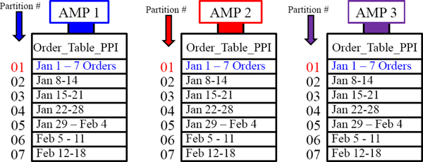
– A Visual of Range_N Partitioning Per Week
– An SQL Example that explains Range_N Partitioning per Day
– Creating a PPI Table with RANGE_N Partitioning per Month
– A Visual of One Year of Data with Range_N Per Month
– An SQL Example explaining Range_N Partitioning per Month
– Creating a PPI Table with CASE_N
– A Visual of Case_N Partitioning
– An SQL Example that explains Range_N Partitioning per Day
– How many partitions do you see?
– Number of PPI Partitions Allowed
– How many partitions do you see?
– NO CASE and UNKNOWN Partitions Together
– A Visual of Case_N Partitioning
– Combining Older Data and Newer Data in PPI
– A Visual for Combining Older Data and Newer Data in PPI
– The SQL on Combining Older Data and Newer Data in PPI
– Multi-Level Partitioning Combining Range_N and Case_N
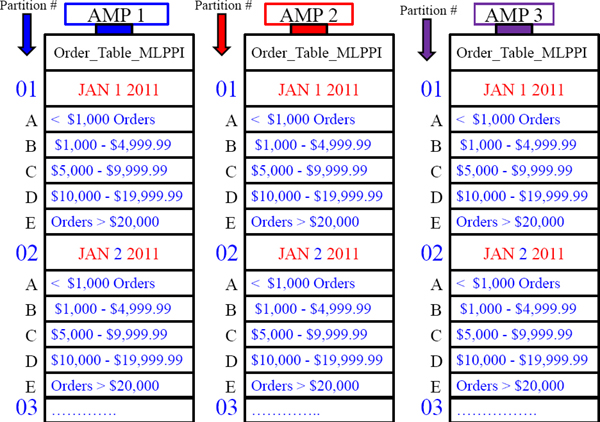
– A Visual of Multi-Level Partitioning
– The SQL on a Multi-Level Partitioned Primary Index
– NON-Unique Primary Indexes (NUPI) in PPI
– PPI Table with a Unique Primary Index (UPI)
– Tricks for Non-Unique Primary Indexes (NUPI)
– Character Based PPI for RANGE_N
– A Visual for Character Based PPI for RANGE_N
– The SQL on Character Based PPI for RANGE_N
– Character Based PPI for CASE_N
– Dates and Character Based Multi-Level PPI
– Using CURRENT_DATE to define a PPI
– ALTER to CURRENT_DATE the next year
– ALTER to CURRENT_DATE with Save
– Altering a PPI Table to Add or Drop Partitions
– Deleting a Partition and Saving its contents
– Using the PARTITION Keyword in your SQL
– Watch the Video on Partitioning
The Concept behind Partitioning a Table
1. Each Table in Teradata has a Primary Index, unless it is a NoPI table.
2. The Primary Index is the mechanism that allows Teradata to physically distribute the rows of a table across the AMPs.
3. AMPs Sort their rows by the Row-ID so the system can perform a lightning fast Binary Search since the rows are in Row-ID Order.
4. Partitioning merely tells the AMP to sort it's tables rows by the Partition first, but then sort the rows by Row-ID within the partition.
5. Partitioning queries will involve All-AMPs, but partitioned tables are designed to prevent FULL Table Scans.
The basic concepts of Partitioning are above so implant these in your mind.
Review of A Unique Primary Index (UPI)
CREATE TABLE Emp_Intl
(Emp_No INTEGER,
Dept_No SMALLINT,
First_Name VARCHAR(12),
Last_Name CHAR(20),
Salary DECIMAL(10,2))
UNIQUE Primary Index( Emp_No)
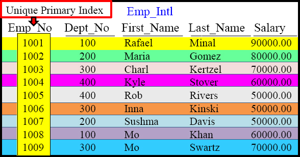

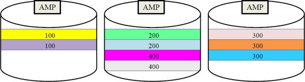
A Unique Primary Index(UPI) spreads the rows of a table evenly across the AMPs.
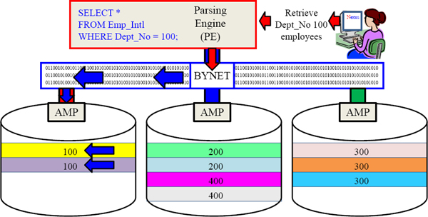
Primary Index in the WHERE Clause – Single-AMP Retrieve
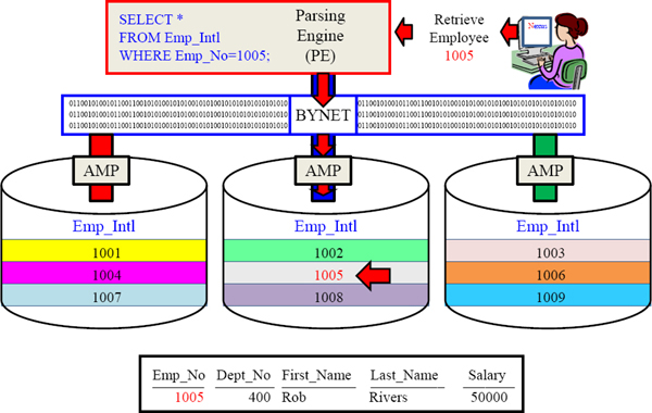
Use the Primary Index column in your SQL WHERE clause and only 1-AMP retrieves.
Review of A Non-Unique Primary Index (NUPI)
CREATE TABLE Emp_Intl
(Emp_No INTEGER,
Dept_No SMALLINT,
First_Name VARCHAR(12),
Last_Name CHAR(20),
Salary DECIMAL(10,2))
Primary Index( Dept_No)
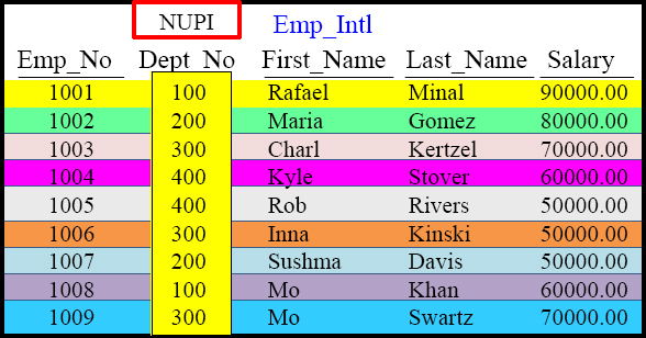
A Non-Unique Primary Index(NUPI) will have duplicates grouped together on the same AMP so data will always be skewed (uneven). The above skew is reasonable and ok.
Primary Index in the WHERE Clause – Single-AMP Retrieve

Use the Primary Index column in your SQL WHERE clause and only 1-AMP retrieves.
Review of a Multi-Column Primary Index
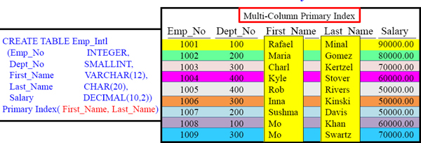

A table can have only one Primary Index, but you can combine up to 64 columns together max to form one Multi-Column Primary Index.
Primary Index in the WHERE Clause – Single-AMP Retrieve
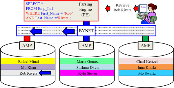

Use the Primary Index column in your SQL WHERE clause and only 1-AMP retrieves.
Creating a PPI Table with Simple Partitioning
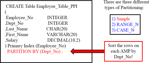
A PPI Table is a table with a Partition on it. A PPI table has the AMPs sort (order ) the rows on the table by the Partition. This allows for people to avoid Full Table Scans. This is an example of Simple PPI. Each AMP will sort the rows they own by Dept_No.
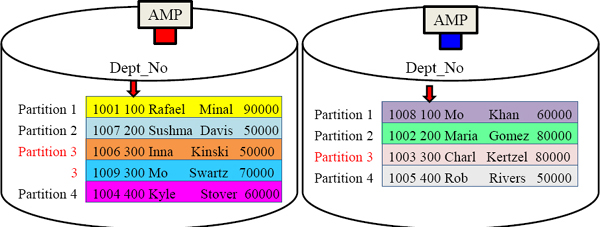
A Visual Display of Simple Partitioning

An SQL Example that explains Simple Partitioning
SQL Query
SELECT *
FROM Employee_Table_PPI
WHERE Dept_No = 300 ;
PE's Explain Plan
We do an All-AMPs
retrieve by way of a
Single Partition.
The table below was Partitioned by Dept_No using Simple Partitioning. Each AMP merely reads from partition 3 which holds all Dept_No 300 employees.
Creating a PPI Table with RANGE_N Partitioning per Day

The above syntax represents a RANGE_N partition.
A Visual of Range_N Partitioning Per Day
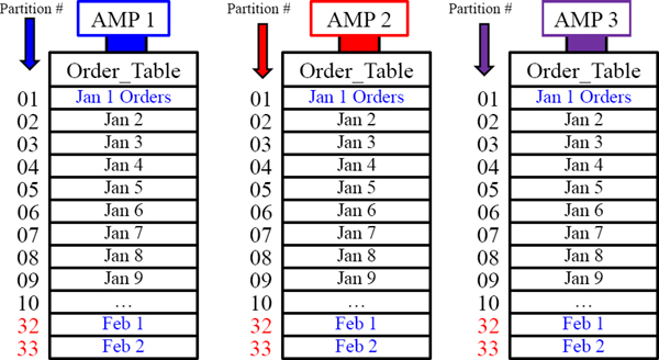
There would be 365 partitions in total for an entire year of Partitioning per Day. Each AMP holds the orders assigned to them in daily partitions on the day of the order date.
An SQL Example that explains Range_N Partitioning per Day
SQL Query
SELECT *
FROM Order_Table_PPI
WHERE Order_Date BETWEEN
‘2012-01-01’ and ‘2012-01-02’ ;
PE's Explain Plan
We do an All-AMPs
retrieve by way of
2 Partitions.
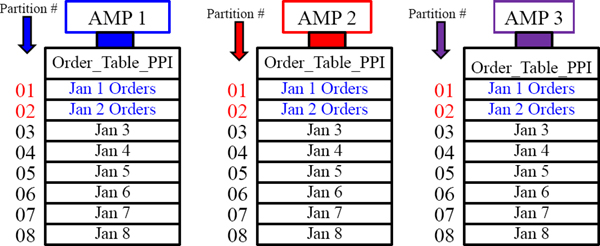
Each AMP holds the orders assigned to them in daily partitions on the day of the order .
Creating a PPI Table with RANGE_N Partitioning per Week
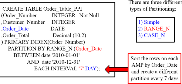
You can order everything by day. You can also order everything by week, my month, and by year. You have many options to choose from.
A Visual of Range_N Partitioning Per Week
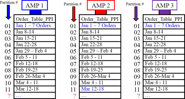
There would be 52 partitions in total for an entire year of Partitioning per Week. Each AMP holds the orders assigned to them in weekly partitions on the week of the order.
An SQL Example that explains Range_N Partitioning per Day
SQL Query
SELECT *
FROM Order_Table_PPI
WHERE Order_Date BETWEEN
‘2012-01-01’ and ‘2012-01-07’ ;
PE's Explain Plan
We do an All-AMPs
retrieve by way of
a single Partition.
Each AMP holds the orders assigned to them in daily partitions on the day of the order .
Creating a PPI Table with RANGE_N Partitioning per Month

You can order everything by day. You can also order everything by week, by month, and by year. You have many options to choose from.
A Visual of One Year of Data with Range_N Per Month

Each AMP sorts their rows by Month (of Order_Date).
An SQL Example explaining Range_N Partitioning per Month
SQL Query
SELECT *
FROM Order_Table
WHERE Order_Date BETWEEN
‘2012-01-01’ and ‘2012-03-31’ ;
PE's Explain Plan
We do an All-AMPs
retrieve by way of
3 Partition3.

The above query wants to see orders in the first quarter so each AMP reads 3 partitions.
Creating a PPI Table with CASE_N
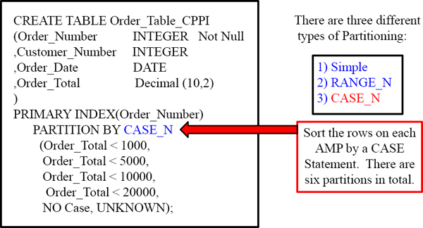
The above syntax represents the CASE_ N partitioning. If an Order_Total is < 1000 it will go into Partition 1. If an Order_Total is between 1000 and 4999.99 it will go in Partition 2. The NO Case partition is for anything falling through and the UNKNOWN partition is for NULL values in the Total.
A Visual of Case_N Partitioning
PARTITION BY CASE_N
(Order_Total < 1000,
Order_Total < 5000,
Order_Total < 10000,
Order_Total < 20000,
NO Case, UNKNOWN);
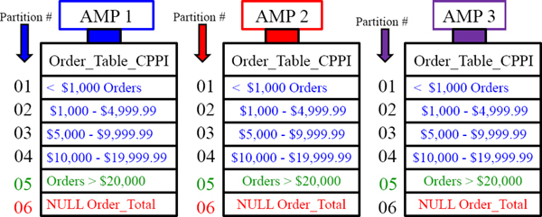
Three are six partitions for this table. Orders are placed in partitions based on cost.
An SQL Example that explains Range_N Partitioning per Day
SQL Query
SELECT *
FROM Order_Table_CPPI
WHERE Order_Total > 20000.00
PE's Explain Plan
We do an All-AMPs
retrieve by way of
a Single Partition.

All-AMPs retrieve but each only reads partition 5 which is a mere sliver of the disk.
How many partitions do you see?
CREATE TABLE Order_Table_PPI
(Order_Number INTEGER Not Null
,Customer_Number INTEGER
,Order_Date DATE
,Order_Total Decimal (10,2)
) PRIMARY INDEX(Order_Number)
PARTITION BY RANGE_N (Order_Date
BETWEEN date '2010-01-01'
AND date '2010-12-31'
EACH INTERVAL '1' DAY);
How many partitions will Order_Table_PPI have at the year's end? It will have 365, unless it is leap year and then it will have 366.
Number of PPI Partitions Allowed
CREATE TABLE Order_Table_PPI
(Order_Number INTEGER Not Null
,Customer_Number INTEGER
,Order_Date DATE
,Order_Total Decimal (10,2)
) PRIMARY INDEX(Order_Number)
PARTITION BY RANGE_N (Order_Date
BETWEEN date '2010-01-01'
AND date '2010-12-31'
EACH INTERVAL '1' DAY);
Each AMP can have 65,535 partitions per table, but after Teradata V14 each AMP can have 9.223 Quintillion partitions per table.
Teradata Tables can have 65,535 partitions max, but after V14 it is 9.223 Quintillion.
How many partitions do you see?
CREATE TABLE Order_Table_CPPI
(Order_Number INTEGER Not Null
,Customer_Number INTEGER
,Order_Date DATE
,Order_Total Decimal (10,2))
PRIMARY INDEX(Order_Number)
PARTITION BY CASE_N
(Order_Total < 1000,
Order_Total < 5000,
Order_Total < 10000,
Order_Total < 20000,
NO Case, UNKNOWN);
How many partitions do you see in the above example?
There are six partitions in the above example. Partition 1 is for Order_Totals < 1000 and Partition 2 is for Order_Totals < 5000, etc. The NO Case partition is for anything falling through the CASE statement, like an ELSE so it is for any Order_Total 20,000 or greater. The UNKNOWN is for Order_Totals that are Null.
NO CASE and UNKNOWN Partitions Together
CREATE TABLE Order_Table_CPPI
(Order_Number INTEGER Not Null
,Customer_Number INTEGER
,Order_Date DATE
,Order_Total Decimal (10,2)
)
PRIMARY INDEX(Order_Number)
PARTITION BY CASE_N
(Order_Total < 1000,
Order_Total < 5000,
Order_Total < 10000,
Order_Total < 20000,
NO Case OR UNKNOWN);
How many partitions do you see in the above example?
There are five partitions in the above example. Partition 1 is for Order-Totals < 1000 and Partition 2 is for Order_Totals < 5000, etc. The NO Case partition and the UNKNOWN partition are combined. So now any Order_Total that is 20,000 or greater or any Order_Total that is NULL will be in the 5th partition together.
A Visual of Case_N Partitioning
PARTITION BY CASE_N
(Order_Total < 1000,
Order_Total < 5000,
Order_Total < 10000,
Order_Total < 20000,
NO CASE OR UNKNOWN);
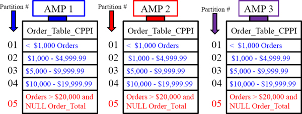
Three are five partitions for this table because we combined the NO CASE and UNKNOWN partitions together. Orders are placed in partitions based on cost.
Combining Older Data and Newer Data in PPI
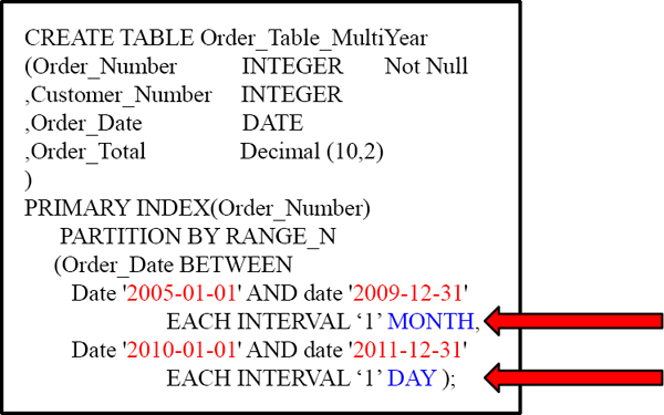
The above example shows Older Data Partitioned by Month and Newer Data by Day.
A Visual for Combining Older Data and Newer Data in PPI
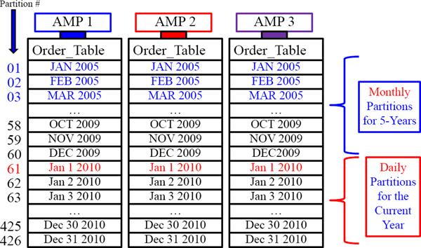
This example combines 5-years of monthly partitions with 1-year of daily partitions.
The SQL on Combining Older Data and Newer Data in PPI
SELECT * FROM Order_Table
WHERE Order_Date BETWEEN‘2010-01-01’ and ‘2010-01-07’ ;
We do an
All-AMPs
retrieve by way
of 7 Partitions.

Multi-Level Partitioning Combining Range_N and Case_N
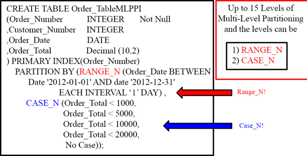
This type of partitioning is called a MULTI-LEVEL PPI. It is a Partition within a Partition. The top partition is the only one you can ALTER so keep that in mind. With Multi-Level partitioning you can combine up to 15 Case_N or Range_N partitions within partitions. NO Simple Partitioning can be used in Multi-Level Partitioning.
A Visual of Multi-Level Partitioning
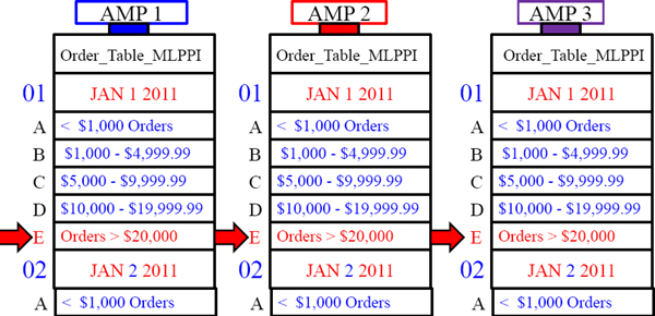
The SQL on a Multi-Level Partitioned Primary Index
SELECT * FROM Order_Table_MLPPI
WHERE Order_Date = ‘2011-01-01’ and Order_Total > 20000 ;
We do an
All-AMPs
retrieve by way
of a Single
Partition.
NON-Unique Primary Indexes (NUPI) in PPI
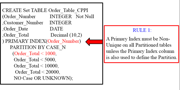
Why were we forced to make the Primary Index of Order_Number a Non-Unique Primary Index (NUPI)? This is because the PRIMARY INDEX (Order_Number ) was not part of the Partition. That is why most PPI tables are defined as NUPI.
PPI Table with a Unique Primary Index (UPI)
CREATE Set TABLE Order_Table_CPPI
(Order_Number INTEGER Not Null
,Customer_Number INTEGER
,Order_Date DATE
,Order_Total Decimal (10,2)
) UNIQUE PRIMARY INDEX(Order_Number, Order_Total)
PARTITION BY CASE_N
(Order_Total < 1000,
Order_Total < 5000,
Order_Total < 10000,
Order_Total < 20000,
NO Case OR UNKNOWN);
We were able to make the Primary Index of (Order_Number, Order_Total) a Unique Primary Index (UPI) because Order_Total was part of the Primary Index and part of the Partition.
Tricks for Non-Unique Primary Indexes (NUPI)

CREATE UNIQUE INDEX(Order_Number)
on Order_Table_Tricks ;
USI
CREATE INDEX(Order_Number)
on Order_Table_Tricks ;
NUSI
You can create a secondary index (USI or NUSI) on the Primary Index to either ensure uniqueness or for faster retrieval. Use either one depending on your needs.
Character Based PPI for RANGE_N
CREATE TABLE Employee_Char
(Employee_No INTEGER
,Dept_No INTEGER
,First_Name CHAR(20)
,Last_Name VARCHAR(20)
,Salary Decimal(10,2)
) PRIMARY INDEX(Employee_No)
PARTITION BY RANGE_N
(Last_Name Between
(‘A’, ‘B’,‘C’, ‘D’, ‘E’, ‘F’, ‘G’, ‘H’, ‘I’,
‘J’, ‘K’,‘L’, ‘M’, ‘N’, ‘O’, ‘P’, ‘Q’, ‘R’,
‘S’, ‘T’,‘U’, ‘V’, ‘W’, ‘X’, ‘Y’, ‘Z’
AND ‘ZZ’, UNKNOWN)) ;
SELECT *
FROM Employee_Table_Char
WHERE Last_Name LIKE ‘C%’ ;
Character Based PPI (Teradata Version 13.10 and beyond) paves the way for Range Queries that are used in conjunction with the LIKE command.
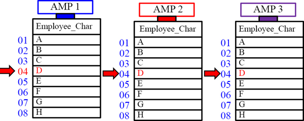
A Visual for Character Based PPI for RANGE_N

Each letter in the alphabet gets their own partition to easily track Last_Name.
The SQL on Character Based PPI for RANGE_N
SELECT * FROM Employee_Char
WHERE Last_Name LIKE ‘DAV%’
We do an All-AMPs retrieve by way of a Single Partition.
Only one partition is read on each AMP and that is the partition for the names that start with the letter ‘D’. The query above finds all last names that start with the letters DAV.
Character Based PPI for CASE_N
CREATE TABLE Product_Table_Char
(Product_ID INTEGER
,Product_Name (CHAR(20)) NOT CASESPECIFIC
,Product_Cost Decimal(10,2)
,Product_Description VARCHAR(100)
) PRIMARY INDEX(Product_ID)
PARTITION BY CASE_N
(Product_Name < ‘Apples’
Product_Name < ‘Bananas’
Product_Name < ‘Cantaloupe’
Product_Name < ‘Grapes’
Product_Name < ‘Lettuce’
Product_Name < ‘Mangos’
Product_Name >= ‘Mangos’ and <= ‘Tomatoes’) ;
SELECT * FROM Product_Table_Char
WHERE Product_Name BETWEEN ‘Apples’ and ‘Grapes’ ;
Character Based PPI (Teradata Version 13.10 and beyond) can use CASE_N.
Dates and Character Based Multi-Level PPI
CREATE TABLE Claims_Table_PPI
(Claim_ID INTEGER NOT NULL
,Claim_Date DATE NOT NULL
,State_ID CHAR(2) NOT NULL
,CL_Details VARCHAR(1000) NOT NULL
) PRIMARY INDEX(Claim_ID)
PARTITION BY (RANGE_N
(Claim_Date BETWEEN DATE ‘2010-01-01’
AND DATE ‘2012-12-31’
EACH INTERVAL ‘1’ DAY)
,RANGE_N (State_ID Between
(‘AL’, ‘AK’,‘AZ’, ‘AR’, ‘CA’, ‘CO’, ‘CT’, ‘DE’, ‘FL’,
‘GA, ’HI’,‘ID’, ‘IL’, ‘IN’, ‘IA’, ‘KS’, ‘KY’, ‘LA’,
‘ME’, ‘MD’,‘MA’, ‘MI’, ‘MN’, ‘MS’, ‘MT’, ‘NE’,
‘NV, ‘NH’,‘NJ’, ‘NM’, ‘NY’, ‘NC’, ‘ND’, ‘OH’, ‘OK’,
‘OR’, ‘PA’,‘RI’, ‘SC’, ‘SD’, ‘TN’, ‘TX’, ‘UT’, ‘VT’,
‘VA’, ‘WA’, ‘WV’, ‘WI’, ‘WY’));
This Multi-Level PPI table uses both Range_N on both Dates and Character based PPI.
TIMESTAMP Partitioning
CREATE TABLE Order_Table_TS
(Order_Number INTEGER NOT NULL
,Customer_Number INTEGER NOT NULL
,Order_Date_Time TIMESTAMP(0) WITH TIME ZONE
,Order_Total Decimal(10,2)
) PRIMARY INDEX(Order_Number)
PARTITION BY (RANGE_N
(CAST (Order_Date_Time as DATE AT 0)
BETWEEN DATE ‘2011-01-01’ AND DATE ‘2011-12-31’
EACH INTERVAL ‘1’ Month ) ;
SELECT * FROM Order_Table_TS
WHERE Order_Date_Time BETWEEN
TIMESTAMP ‘2011-01-13 00:00:00-08:00’ AND
TIMESTAMP ‘2011-01-13 23:59:59-08:00’ ;
Find all Orders Place on the day January 13, 2011
TIMESTAMP partitioning is available with Teradata V13.10. Notice the DATE at 0 in the CREATE statement. This means the Timestamp is Deterministic, which means the system will know your Time Zone and retrieve the rows from your point of time.
Using CURRENT_DATE to define a PPI
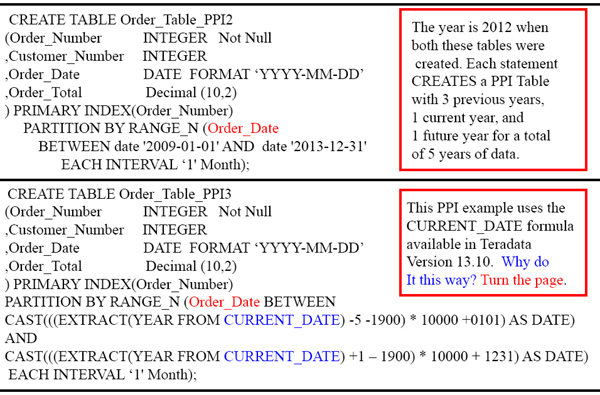
Both CREATE statements above demand 5 years of partitioned data from 2009-2013.
ALTER to CURRENT_DATE the next year
In Teradata V13.10 the system allowed for CURRENT_DATE to be utilized in the PPI CREATE statement. This allowed for easy altering of the data and deleting of partitions. The ALTER Table command can alter to reflect 5 years, now going from 1010-2014.
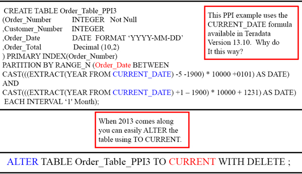
ALTER to CURRENT_DATE with Save

When 2013 comes along you can easily ALTER the table using TO CURRENT.
ALTER TABLE Order_Table_PPI3 TO CURRENT WITH INSERT INTO Order_Table_History ;
Notice we are ALTERING the table to CURRENT, but instead of deleting the data we are moving the old data into a History file called Order_Table_History.
Altering a PPI Table to Add or Drop Partitions
Creating a PPI Table
CREATE TABLE Order_TablePPI
(Order_Number INTEGER Not Null
,Customer_Number INTEGER
,Order_Date DATE
,Order_Total Decimal (10,2))
PRIMARY INDEX(Order_Number)
PARTITION BY RANGE_N
(Order_Date BETWEEN
date '2010-01-01'
AND date '2010-12-31'
EACH INTERVAL ‘1’ DAY);
ALTERING a PPI Table
ALTER TABLE Order_TablePPI
MODIFY PRIMARY INDEX
DROP RANGE BETWEEN
DATE ‘2010-01-01’
AND DATE ‘2010-12-31’
EACH INTERVAL ‘1’ DAY
ADD RANGE BETWEEN
DATE ‘2011-01-01’
AND DATE ‘2011-12-31’
EACH INTERVAL ‘1’ DAY
WITH DELETE ;
What will happen to the 2010 data after the ALTER?
Deleting a Partition
Creating a PPI Table
CREATE TABLE Order_TablePPI
(Order_Number INTEGER Not Null
,Customer_Number INTEGER
,Order_Date DATE
,Order_Total Decimal (10,2))
PRIMARY INDEX(Order_Number)
PARTITION BY RANGE_N
(Order_Date BETWEEN
date '2010-01-01'
AND date '2010-12-31'
EACH INTERVAL ‘1’ DAY);
ALTERING a PPI Table
ALTER TABLE Order_TablePPI
MODIFY PRIMARY INDEX
DROP RANGE BETWEEN
DATE ‘2010-01-01’
AND DATE ‘2010-12-31’
EACH INTERVAL ‘1’ DAY
ADD RANGE BETWEEN
DATE ‘2011-01-01’
AND DATE ‘2011-12-31’
EACH INTERVAL ‘1’ DAY
WITH DELETE ;
The 2010 data after the ALTER will be deleted from the table.
Deleting a Partition and Saving its contents
Creating a PPI Table
CREATE TABLE Order_TablePPI
(Order_Number INTEGER Not Null
,Customer_Number INTEGER
,Order_Date DATE
,Order_Total Decimal (10,2))
PRIMARY INDEX(Order_Number)
PARTITION BY RANGE_N
(Order_Date BETWEEN
date '2010-01-01'
AND date '2010-12-31'
EACH INTERVAL ‘1’ DAY);
ALTERING a PPI Table
ALTER TABLE Order_TablePPI
MODIFY PRIMARY INDEX
DROP RANGE BETWEEN
DATE ‘2010-01-01’
AND DATE ‘2010-12-31’
EACH INTERVAL ‘1’ DAY
ADD RANGE BETWEEN
DATE ‘2011-01-01’
AND DATE ‘2011-12-31’
EACH INTERVAL ‘1’ DAY
WITH INSERT INTO
Order_Table_History ;
The 2010 data after the ALTER will be deleted from the table, but the deleted data is stored in Order_Table_History.
Using the PARTITION Keyword in your SQL
SELECT PARTITION as “Partition Number”
,Count(*) as “Rows in Partition”
FROM Order_Table_PPI
GROUP BY 1
ORDER BY 1 ;
| Partition Number | Rows in Partition |
| 1 | 1000 |
| 2 | 1200 |
| 3 | 1100 |
| 4 | 1022 |
| 5 | 1121 |
| 6 | 1132 |
| 7 | 1300 |
| 8 | 1500 |
| 9 | 1610 |
You can find out how many partitions you have and the number of rows from the above query. You won't see information about empty partitions.
SQL for RANGE_N
SELECT RANGE_N (
Calendar_Date BETWEEN DATE ‘2010-01-01’ AND DATE ‘2010-04-30’
EACH INTERVAL ‘1’ MONTH) AS “Partition”
,MIN(Calendar_Date) as “Begin Date”
,MAX(Calendar_Date) as “End Date”
FROM Sys_Calendar.Calendar
WHERE Calendar_Date BETWEEN DATE ‘2010-01-01’ and DATE ‘2010-04-30’
GROUP BY 1
ORDER BY 1 ;
| Partition | Begin Date | End Date |
| 1 | 2010-01-01 | 2010-01-31 |
| 2 | 2010-02-01 | 2010-02-28 |
| 3 | 2010-03-01 | 2010-03-31 |
| 4 | 2010-04-01 | 2010-04-30 |
You can find out how many partitions you have and the number of rows from the above query. You won't see information about empty partitions.
SQL for CASE_N
SELECT CASE_N (
Order_Total < 1000
,Order_Total < 5000
,Order_Total < 10000
,Order_Total < 20000
,NO Case
,UNKNOWN) as “Partition”
,COUNT(*) as “Counter”
FROM Order_Table_PPI
GROUP BY 1
ORDER BY 1 ;
| Partition | Counter |
| 1 | 100 |
| 2 | 125 |
| 3 | 140 |
| 4 | 110 |
| 5 | 3 |
You can find out how many partitions you have and the number of rows from the above query. You won't see information about empty partitions.
Watch the Video on Partitioning

Tera-Tom Trivia
Tom Coffing graduated with a Bachelor's degree in Speech Communications. Tom spent 10 years in Toastmasters competing in hundreds of speech contests. Tom won speech championships at the city, area, state, and national level.
Click on the link below or place it in your browser and watch the video on partitioning.