
CHAPTER 9
INTRODUCTION TO STOCHASTIC PROCESSES
In the last eight chapters, we have studied probability theory, which is the mathematical study of random phenomena. A random phenomenon occurs through a stochastic process. In this chapter we introduce stochastic processes that can be defined as a collection of random variables indexed by some parameter. The parameters could be time (or length, weight, size, etc.). The word “stochastic1” means random or chance. The theory of stochastic processes turns out to be a useful tool in solving problems belonging to diverse disciplines such as engineering, genetics, statistics, economics, finance, etc. This chapter discusses Markov chains, Poisson processes, and renewal processes. In the next chapter, we introduce some important stochastic processes for financial mathematics, Wiener processes, martingales, and stochastic integrals.
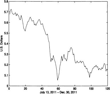
Figure 9.1 Sample path for the U.S. dollar value of 10,000 Colombian pesos
9.1 DEFINITIONS AND PROPERTIES
Definition 9.1 (Stochastic Process) A real stochastic process is a collection of random variables {Xt; t ![]() T} defined on a common probability space
T} defined on a common probability space ![]() with values in
with values in ![]() . T is called the index set of the process or parametric space, which is usually a subset of
. T is called the index set of the process or parametric space, which is usually a subset of ![]() . The set of values that the random variable Xt can take is called the state space of the process and is denoted by S.
. The set of values that the random variable Xt can take is called the state space of the process and is denoted by S.
The mapping defined for each fixed ![]() ,
,
![]()
is called a sample path of the process over time or a realization of the stochastic process.
The U.S. dollar value of 10,000 Colombian pesos at the end of each day is a stochastic process {Xt; t ![]() T}. The sample path of {Xt; t
T}. The sample path of {Xt; t ![]() T} between July 13, 2011 and December 30, 2011, is shown in Figure 9.1.
T} between July 13, 2011 and December 30, 2011, is shown in Figure 9.1. ![]()
Stochastic processes are classified into four types, depending upon the nature of the state space and parameter space, as follows:
1. Discrete-state, discrete-time stochastic process
(a) The number of individuals in a population at the end of year t can be modeled as a stochastic process {Xt;t ![]() T}, where the index set T = {0, 1, 2, …} and the state space S = {0,1, 2, …}.
T}, where the index set T = {0, 1, 2, …} and the state space S = {0,1, 2, …}.
(b) A motor insurance company reviews the status of its customers yearly. Three levels of discounts are possible (0, 10%, 25%) depending on the accident record of the driver. Let Xt be the percentage of discount at the end of year t. Then the stochastic process {Xt;t ![]() T} has T = {0, 1, 2, …} and S = {0, 10, 25}.
T} has T = {0, 1, 2, …} and S = {0, 10, 25}.
2. Discrete-state, continuous-time stochastic process
(a) The number of incoming calls Xt in an interval [0, t]. Then the stochastic processes {Xt;t ![]() T} has T = {t : 0 ≤ t < ∞} and S = {0, 1, 2, …}.
T} has T = {t : 0 ≤ t < ∞} and S = {0, 1, 2, …}.
(b) The number of cars Xt parked at a commercial center in the time interval [0,t]. Then the stochastic processes {Xt; t ![]() T} has T = {t : 0 ≤ t < ∞} and S = {0, 1, …}.
T} has T = {t : 0 ≤ t < ∞} and S = {0, 1, …}.
3. Continuous-state, discrete-time stochastic process
(a) The share price for an asset at the close of trading on day t with T = {0, 1, 2, …} and S = {x : 0 ≤ x < ∞}. Then it is a discretetime stochastic process with the continuous-state space.
4. Continuous-state, continuous-time stochastic process
(a) The value of the Dow-Jones index at time t where T = {t : 0 ≤ t < ∞} and S = {x : 0 ≤ x < ∞}. Then it is a continuous-time stochastic process with the continuous-state space. ![]()
Definition 9.2 (Finite-Dimensional Distributions of the Process) Let {Xt; t ![]() T} be a stochastic process and {t1, t2, … ,tn}
T} be a stochastic process and {t1, t2, … ,tn} ![]() T where t1 < t2 < … < tn. The finite dimensional distribution of the process is defined by:
T where t1 < t2 < … < tn. The finite dimensional distribution of the process is defined by:
![]()
The family of all finite-dimensional distributions determines many important properties of the stochastic process. Under some conditions it is possible to show that a stochastic process is uniquely determined by its finitedimensional distributions (advanced reader may refer to Breiman, 1992).
We now discuss a few important characteristics and classes of stochastic processes.
Definition 9.3 (Independent Increments) If, for all t0, t1, t2, … tn such that t0 < t1 < t2 < … < tn, the random variables Xt0, Xt1 − Xt0, Xt2 − Xt1, … , Xtn − Xtn−1 are independent (or equivalently Xt+r − Xr is independent of Xs for s < τ), then the process {Xt; t ![]() T} is said to be a process with independent increments.
T} is said to be a process with independent increments.
Definition 9.4 (Stationary Increments) A stochastic process {Xt; t ![]() T} is said to have stationary increments if Xt2+τ − Xt1+τ has the same distribution as Xt2 − Xt1 for all choices of t1, t2 and τ > 0.
T} is said to have stationary increments if Xt2+τ − Xt1+τ has the same distribution as Xt2 − Xt1 for all choices of t1, t2 and τ > 0.
Definition 9.5 (Stationary Process) If for arbitrary t1, t2, …, tn, such that t1 < t2 < … < tn, the joint distributions of the vector random variables (Xt1, Xt2, …, Xtn) and (Xt1+h, Xt2+h, … Xtn+h) are the same for all h > 0, then the stochastic process {Xt; t ![]() T} is said to be a stationary stochastic process of order n (or simply a stationary process). The stochastic process {Xt; t
T} is said to be a stationary stochastic process of order n (or simply a stationary process). The stochastic process {Xt; t ![]() T} is said to be a strong stationary stochastic process or strictly stationary process if the above property is satisfied for all n.
T} is said to be a strong stationary stochastic process or strictly stationary process if the above property is satisfied for all n.
Suppose that {Xn; n ≥ 1} is a sequence of independent and identically distributed random variables. We define the sequence {Yn; n ≥ 1} as
![]()
where a is a real constant. Then it is easily seen that {Yn; n ≥ 1} is strictly stationary. ![]()
Definition 9.6 (Second-Order Process) A stochastic process {Xt; t ![]() T} is called a second-order process if E ((Xt)2) < ∞ for all t
T} is called a second-order process if E ((Xt)2) < ∞ for all t ![]() T.
T.
Let Z1 and Z2 be independent normally distributed random variables, each having mean 0 and variance σ2. Let ![]() and:
and:
![]()
{Xt; t ![]() T} is a second-order stationary process.
T} is a second-order stationary process. ![]()
Definition 9.7 (Covariance Stationary Process) A second-order stochastic process {Xt; t ![]() T} is called covariance stationary or weakly stationary if its mean function m(t) = E[Xt] is independent of t and its covariance function Cov(Xs, Xt) depends only on the difference |t − s| for all s, t
T} is called covariance stationary or weakly stationary if its mean function m(t) = E[Xt] is independent of t and its covariance function Cov(Xs, Xt) depends only on the difference |t − s| for all s, t ![]() T. That is:
T. That is:
![]()
Let {Xn; n ≥ 1} be uncorrelated random variables with mean 0 and variance 1. Then Cov(Xm, Xn) = E(Xm Xn) equals 0 if m ≠ n and 1 if m = n. Then this shows that {Xn; n ≥ 1} is a covariance stationary process. ![]()
Definition 9.8 (Evolutionary Process) A stochastic process which is not stationary (in any sense) is said to be an evolutionary stochastic process.
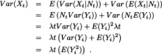
Consider the process {Xt; t ≥ 0}, where Xt = A1 + A2t + A1 and A2 are independent random variables with E(Ai) = μi, ![]() for i = 1,2. It easy to see that:
for i = 1,2. It easy to see that:

These are functions of t and the process is evolutionary. ![]()
The class of processes defined below, known as Markov processes is a very important process both in applications as well as in the development of the theory of stochastic processes.
Definition 9.9 (Markov Process) Let {Xt t ≥ 0} be a stochastic process defined over a probability space ![]() and with state space
and with state space ![]() . We say that {Xt t ≥ 0} is a Markov process if for any 0 ≤ t1 < t2 < … < tn and for any B
. We say that {Xt t ≥ 0} is a Markov process if for any 0 ≤ t1 < t2 < … < tn and for any B ![]()
![]() :
:
![]()
1. Roughly a Markov process is a process such that, given the value Xs, the distribution of Xt for t > s does not depend on the values of Xu, u < s.
2. Any stochastic process which has independent increments is a Markov process.
A discrete-state Markov process is known as a Markov chain. Based on the values of the index set T, the Markov chain is classified as a discrete-time Markov chain (DTMC) or a continuous-time Markov chain (CTMC).
In the next section we will work with discrete-time parameter Markov processes and with discrete-state space, that is, we will continue our study of the so-called Markov chains with discrete-time parameter.
9.2 DISCRETE-TIME MARKOV CHAIN
This section intends to present the basic concepts and theorems related to the theory of discrete-time Markov chains with examples. This section was inspired by the class notes of the courses Stochastik I und II given by Professor H. J. Schuh at the Johannes Gutenberg Universität (Mainz, Germany).
Definition 9.10 (Discrete-Time Markov Chain) A sequence of random variables ![]() with discrete-state space is called a discrete-time Markov chain if it satisfies the conditions
with discrete-state space is called a discrete-time Markov chain if it satisfies the conditions
for all ![]() and for all i0, i1, …, in−1, i, j
and for all i0, i1, …, in−1, i, j ![]() S with:
S with:
![]()
In other words, the condition (9.1) implies the following: if we know the present state “Xn = i″, the knowledge of past history “Xn−1, Xn−2, …, X0 ”has no influence on the probabilistic structure of the future state Xn+1.
Suppose that a coin is tossed repeatedly and let:
Xn := “number of heads obtained in the first n tosses”.
It is clear that the number of heads obtained in the first n + 1 tosses only depends on the knowledge of the number of heads obtained in the first n tosses and therefore:
![]()
for all ![]() and for all i, j, in−1, …, i1
and for all i, j, in−1, …, i1 ![]()
![]() .
. ![]()
Three boys A, B and C throw a ball to each other. A always throws the ball to B and B always throws the ball to C where C is equally likely to throw the ball to A or B. Let Xn := “the boy who has the ball in the nth throw”. The state space of the process is S = {A, B, C} and it is clear that {Xn; n ≥ 0} is a Markov chain, since the person throwing the ball is not influenced by those who previously had the ball. ![]()
Consider a school which consists of 400 students with 250 of them being boys and 150 girls. Suppose that the students are chosen randomly one followed by the other for a medical examination. Let Xn be the sex of the nth student chosen. It is easy to see that {Xn; n = 1, 2, …, 400} is not a discrete-time Markov chain. ![]()
Let Y0, Y1, …, Yn be nonnegative, independent and identically distributed random variables. The sequence {Xn; n ≥ 0} with
![]()
is a Markov chain because:

![]() EXAMPLE 9.11 A Simple Queueing Model
EXAMPLE 9.11 A Simple Queueing Model
Let 0, 1, 2, … be the times at which an elevator starts. It is assumed that the elevator can transport only one person at a time. Between the times n and n + 1, Yn people who want to get into the elevator arrive. Also assume that the random variables Yn, n = 0,1,2, …, are independent. The queue length Xn immediately before the start of the elevator at time n is equal to:
![]()
Suppose that X0 = 0. Since Xi with i ≤ n can be expressed in terms of Y1, Y2, …, Yn−1, we have that Yn is independent of (X0, X1, …, Xn) as well. Thus:
1. If in ≥ 1, then:

The second equality follows from the fact that in ≥ 1, then in+1 = Xn+1 = Xn − 1 + Yn, which implies that Yn = in+1 − Xn + 1.
2. If in = 0, then Xn+1 = Yn, and in this case:

Lemma 9.1 If {Xn; n ≥ 0} is a Markov chain, then for all n and for all i0, i1, …, in ![]() S we have:
S we have:
![]()
Proof:

![]()
The previous lemma states that to know the joint distribution of X0, X1, …, Xn, it is enough to know P(X0 = i0), P(X1 = i1 | X0 = i0), etc. Moreover, for any finite set {j1, j2, …, jl} of subindices, any probability that involves the variables Xj1, Xj2, …, Xjl with j1 < j2 < … < jl, l = 1,2, …, n, can be obtained from:
![]()
Then it follows that one can know the joint distribution of the random variables Xj1, Xj2, …, Xjl from the knowledge of the values of P(X0 = i0), P(X1 = i1 | X0 = i0), etc. These probabilities are so important that they have a special name.
Definition 9.11 (Transition Probability) Let {Xn; n ≥ 0} be a Markov chain. The probabilities
![]()
(if defined) are called transition probabilities.
Definition 9.12 A Markov chain {Xn; n ≥ 0} is called homogeneous or a Markov chain with stationary probabilities if the transition probabilities do not depend on n.
Note 9.2 In this book we only consider homogeneous Markov chains unless otherwise specially mentioned.
Definition 9.13 The probability distribution ![]() with
with
![]()
is called the initial distribution.
Because of the dual subscripts it is convenient to arrange the transition probabilities in a matrix form.
Definition 9.14 (Transition Probability Matrix) The matrix
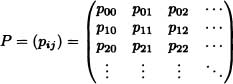
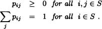
is called the transition probability matrix or stochastic matrix. Note that:
From Example 9.11 we have that:
![]()
If we define pj := P(Yn = j), then the transition probability matrix P of the Markov chain is given by:

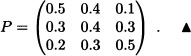
On any given day Gary is cheerful (C), normal (N) or depressed (D). If he is cheerful today, then he will be C, N or D tomorrow with probabilities 0.5, 0.4, 0.1, respectively. If he is feeling so-so today, then he will be C, N or D tomorrow with probabilities 0.3, 0.4, 0.3. If he is glum today, then he will be C, N, or D tomorrow with probabilities 0.2, 0.3, 0.5. Let Xn denote Gary’s mood on the nth day. Then {Xn; n ≥ 0} is a three-state discrete-time Markov chain (state 0 = C, state 1 = N, state 2 = D) with transition probability matrix
![]() EXAMPLE 9.14 Simple Random Walk Model
EXAMPLE 9.14 Simple Random Walk Model
A discrete-time Markov chain whose state space is given by the integers i = 0, ±1, ±2, … is said to be a random walk if for some number 0 < p < 1:
![]()
The preceding DTMC is called a simple random walk for we may think of it as being a model for an individual walking on a straight line who at each point of time either takes one step to the right with probability p or one step to the left with probability 1 − p. The one-step transition probability matrix is given by:

Suppose that we have two players A and B and that player A who started a game has a capital of x ![]()
![]() dollars and player B has a capital of y
dollars and player B has a capital of y ![]()
![]() dollars. Let a := x + y. In each round of the game, either A wins one dollar from B with probability p or B wins one dollar from A with probability q, with p + q = 1. The game goes on until one of the players loses all of his capital, that is, until Xn = 0 or Xn = a, since Xn = “The capital of the player A in the nth round”. In this case we have T =
dollars. Let a := x + y. In each round of the game, either A wins one dollar from B with probability p or B wins one dollar from A with probability q, with p + q = 1. The game goes on until one of the players loses all of his capital, that is, until Xn = 0 or Xn = a, since Xn = “The capital of the player A in the nth round”. In this case we have T = ![]() and S = {0, 1, …, a}. It is easy to verify that {Xn; n ≥ 0} is a Markov chain. Next, we will see its initial distribution and transition matrix. We have that P(X0 = x) = 1, and hence
and S = {0, 1, …, a}. It is easy to verify that {Xn; n ≥ 0} is a Markov chain. Next, we will see its initial distribution and transition matrix. We have that P(X0 = x) = 1, and hence
![]()
where the 1 appears in the xth component and the matrix P is equal to:

Let {Xn; n ≥ 0} be a Markov chain with states 0,1,2 and with transition probability matrix
The initial distribution is ![]() , i = 0, 1, 2. Then:
, i = 0, 1, 2. Then:

We now explain how Markov chains can be represented as graphs. In a Markov chain, a set of states can be represented by a “network” in which states are vertices and one-step transitions between states are represented by directed arcs. Each of the transitions corresponds to a probability. This graphical representation for the Markov chain is called a state transition diagram. If for some transition the probability of occurrence is zero, then it indicates that the transition is not possible and the corresponding arc is not drawn.
For example, if {Xn; n ≥ 1} is a Markov chain with S = {0, 1, 2, 3} and transition probability matrix

then the state transition diagram is shown in Figure 9.2. In the study of Markov chains the following equations, called Chapman-Kolmogorov equations are very important.
Theorem 9.1 (Chapman-Kolmogorov Equations) If the sequence of random variables {Xn; n ≥ 0} is a Markov chain and if k < m < n, then we have for all h, j ![]() S:
S:
![]()
Proof:


Figure 9.2 State transition diagram
That is:

To give an interpretation to the Chapman-Kolmogorov equations, we introduce the following concept:
Definition 9.15 The probability
![]()
is the m-step transition probability from i to j:
![]()
where δij is Kronecker’s delta. The matrix ![]() is the m-step transition matrix.
is the m-step transition matrix.
Consider the simple random walk of Example 9.14. The state transition diagram is shown in Figure 9.3. Assume that the process starts at the

Figure 9.3 State transition diagram
origin. We have:
![]()
This can be seen by noting that there will be ![]() positive steps and
positive steps and ![]() negative steps in order to go from state i to j in n steps when n + j − i is even.
negative steps in order to go from state i to j in n steps when n + j − i is even. ![]()
Corollary 9.1 The m-step transition probability matrix is the mth power of the transition matrix P.
Corollary 9.2 Let {Xn; n ≥ 0} be a Markov chain with transition probability matrix P and initial distribution π. Then for each n ≥ 1 and for each k ![]() S we have:
S we have:
![]()
Proof:

Note 9.3 The Chapman-Kolmogorov equations provide a procedure to compute the n-step transition probabilities. Indeed it follows that:
![]()
In matrix form, we can write these as
![]()
where · denotes matrix multiplication. Here, P(n) is the matrix consisting of n-step transition probabilities.
Note that beginning with
![]()
and continuing by induction, we can show that the n-step transition matrix can be obtained by multiplying matrix P by itself n times, that is:
![]()
Let {Xn; n ≥ 1} be a Markov chain with state space S = {0,1}, initial distribution ![]() and transition matrix
and transition matrix
![]()
Then
![]()
with
![]()
so that:
![]()
9.2.1 Classification of States
One of the fundamental problems in the study of Markov chains is the analysis of its asymptotic behavior. As we will see later, it depends on whether the chain returns to its starting point with probability 1 or not. For this analysis we need to classify the states, which is the objective of this section.
Definition 9.16 (Accessibility) State j is said to be accessible from state i in n ≥ 0 steps ![]() . This is written as i → j[n]. We say that state j is accessible from state i if there exists n ≥ 0 such that
. This is written as i → j[n]. We say that state j is accessible from state i if there exists n ≥ 0 such that ![]() . In this case we write i → j.
. In this case we write i → j.
Lemma 9.2 The relation “→” is transitive.
Proof: Suppose that i → j and j → k. Then there exist nonnegative integers r and I such that:
![]()
From the Chapman-Kolmogorov equation, we have:
![]()
Therefore, i→ k. ![]()
Definition 9.17 States i and j communicate if i → j and j → i. This is written as i ↔ j.
It is easy to verify that “i ↔ j” is an equivalence relation over S and thus the equivalence classes
![]() ,
,
form a partition of S.
Definition 9.18 A Markov chain is said to be irreducible if the state space consists of only one class, that is, all states communicate with each other.
A Markov chain for which there is only one communication class is called an irreducible Markov chain: Note that, in this case, all states communicate.
Let {Xn;n ≥ 0} be a Markov chain with state space S = {1,2,3}, initial distribution π = (1,0,0) and transition matrix

It is to be observed that C(l) = C(2) = C(3) = {1,2,3}, that is, (Xn)n≥0 is an irreducible Markov chain. ![]()
Definition 9.19 (Absorbing State) A state i is said to be an absorbing state if pii = 1 or equivalently pij = 0 for all j ≠ i.
Consider a Markov chain consisting of the four states 0, 1, 2, 3 and having transition probability matrix


Figure 9.4 State transition diagram for Example 9.20
The state transition diagram for this Markov chain is shown in Figure 9.4. The classes of this Markov chain are {0,1} and {3}. Note that while state 0 (or 1) is accessible from state 2, the reverse is not true. Since state 3 is an absorbing state, that is, p33 = 1, no other state is accessible from it. ![]()
Definition 9.20 Let i ![]() S fixed. The period of i is defined as follows:
S fixed. The period of i is defined as follows:
![]() .
.
where GCD stands for greatest common divisor. If ![]() = 0 for all n ≥ 1, then we define λ(i) := 0.
= 0 for all n ≥ 1, then we define λ(i) := 0.
Definition 9.21 (Aperiodic) State i is called aperiodic when λ (i) = 1.
Definition 9.22 A Markov chain with all states aperiodic is called an aperiodic Markov chain.
In the example of the gambler’s ruin, we have that:

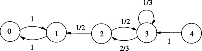
Figure 9.5 State transition diagram for Example 9.22
The following theorem states that if two states are communicating with each other, then they have the same period. ![]()
Theorem 9.2 If i ↔ j, then λ (i) = λ (j).
Proof: Suppose that j → j[n] and let k, m ![]() such that i → j[k] and j → i[m]. Then i → i[m + k] and i → i[m + n + k]. Therefore, λ (i) divides both m + k and m + n + k and from this it follows that λ (i) divides n. That is, λ (i) is a common divisor for all n such that j → j[n] and this implies that λ(i) ≤ λ(j). Similarly it can be shown that λ(j) ≤ λ(i).
such that i → j[k] and j → i[m]. Then i → i[m + k] and i → i[m + n + k]. Therefore, λ (i) divides both m + k and m + n + k and from this it follows that λ (i) divides n. That is, λ (i) is a common divisor for all n such that j → j[n] and this implies that λ(i) ≤ λ(j). Similarly it can be shown that λ(j) ≤ λ(i). ![]()
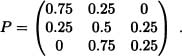
Let {Xn;n ≥ 1} be a Markov chain with state space S = {0,1,2,3,4} and transition matrix

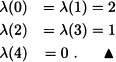
The graphical representation of the chain is shown in Figure 9.5. Then:
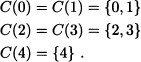
It is clear that:
Suppose that the Markov chain {Xn;n ≥ 0} starts with the state j. Let τk be the first passage time to state k:
τk = min{n ≥ 1 : Xn = k}.
If {n ≥ 1 : Xn = k} = ![]() , we define τk = ∞. For n ≥ 1, define:
, we define τk = ∞. For n ≥ 1, define:
![]()
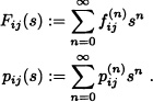
Let ![]() be the probability that the chain reaches the state k (not necessarily for the first time) after n transitions. A relation between
be the probability that the chain reaches the state k (not necessarily for the first time) after n transitions. A relation between ![]() and
and ![]() is as follows.
is as follows.
Theorem 9.3 (First Entrance Theorem)
where ![]() .
.
If j = k we refer to ![]() as the probability that the first return to state j occurs at time n. By definition, we have
as the probability that the first return to state j occurs at time n. By definition, we have ![]() = 0.
= 0.
For fixed states j and k, we have
which is the probability that starting with state j the system ever reaches state k. If j = k, we let fjj = ![]() to denote the probability of ultimately returning to state j.
to denote the probability of ultimately returning to state j.
Definition 9.23 (Recurrent State) A state j is said to be persistent or recurrent if fjj = 1 (i.e., return to state j is certain).
Definition 9.24 (Transient State) A state j is said to be transient if fjj < 1 (i.e., return to state j is uncertain).
Consider the Markov chain with state space S = {0,1,2,3} and transition matrix
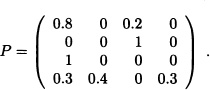

Figure 9.6 State transition diagram for Example 9.23
The state transition diagram for this Markov chain is shown in Figure 9.6.
In this case:
 .
.
We have C(0) = {0,2}, C(1) = {1}, C(3) = {3}. The states 0 and 2 are recurrent and states 1 and 3 are transient. ![]()
Consider the Maxkov chain with state space S = {1,2,3,4,5} and transition matrix
In this case, using Definition 9.17, C(1) = {1,3,4}, C(2) = {2,5}. All the states are recurrent. ![]()
Note 9.4 The transition matrix of a finite Markov chain can always be written in the form
where R corresponds to the submatrix that gives the probability of transition between recurrent states, A is the submatrix whose components are the probabilities of transition from transient states to recurrent states, 0 is the zero matrix and B is the submatrix of transition probabilities between transient states. If among the recurrent states there is an absorbing state, it is placed first in this reordering of the states. This representation of the transition matrix is known as the canonical form of the transition matrix.
Consider the Markov chain with state space S = {0,1,2,3} and transition matrix

We have the canonical form of the transition matrix:

Note 9.5 In the study of finite Markov chains, we are interested in answering questions such as:
1. What is the probability that starting from a transient state i, the chain reaches the recurrent state j at least once?
2. Given that the chain is in a transient state, what is the mean number of visits to another transient state j before reaching a recurrent state?
To answer these questions we introduce some results (without proof). The interested reader may refer to Bhat and Miller (2002).
Definition 9.25 (Fundamental Matrix) The matrix M = (I – B)–l, as in (9.4), is called the fundamental matrix.
Theorem 9.4 For a finite Markov chain with transition matrix P partitioned as (9.4), we have that (I – B)–1 exists and is equal to:
![]()
Proof: we have
and since Bn ![]() 0, then:
0, then:
![]()
Thus for sufficient large n, we have that det (I – Bn) ≠ 0 and consequently
det ((I – B)(I + B + … + Bn–1)) ≠ 0
so that det(I – B) ≠ 0, which implies that (I – B)–l exists.
Multiplying (9.5) by (I – B)–1 we obtain
I + B + … + Bn–1 = (I – B)–1(I – Bn)
and thus, letting n tend to ∞, we get:
![]()
![]()
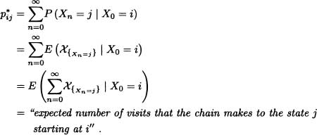
Definition 9.26 Let i,j be transient states. Suppose that the chain starts from the state i and let Nij be the random variable defined as: Nij = “The number of times the chain visits state j before reaching possibly a recurrent state”. We define:
μij = E(Nij).
Theorem 9.5 Let i,j ![]() T where T denotes the set of transient states. Then the fundamental matrix M is given by:
T where T denotes the set of transient states. Then the fundamental matrix M is given by:
![]()
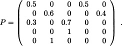
Let us consider a Markov chain with states space S = {0,1,2,3} and probability transition matrix

For a Markov chain, starting from state 0, determine the expected number of visits that the chain makes to state 0 before reaching a recurrent class.
Solution: It can be easily seen that the chain classes are given by C(2) = {2,3} and C(0) = {0,1}, the transient states are 0 and 1 and the recurrent states are 2 and 3. Recognizing matrix P (with the order of states 2301) we have:

That is,
![]()
and:

Hence, ![]()
Definition 9.27 gij is the probability that starting from the transient state i the chain reaches the recurrent state j at least once. We define:
G = (gij).
Theorem 9.6 Let M and A be the matrices defined earlier. Then the matrix G defined above satisfies the relation
G = M A.
Consider the education process of a student after schooling. The student begins with a bachelor’s program and after its completion, proceeds to a master’s program. On completion of the bachelor’s program, the student can join job A whereas on completion of the master’s program, the student joins job B. The education of the student is modeled as a stochastic process {Xt;t ≥ 0} with state space S = {0,1,2,3,4} where states 0, 1 and 2 represent the stages of educational qualification achieved in chronological order and states 3 and 4 represent job A and job B, respectively. The corresponding state transition diagram is shown in Figure 9.7

Figure 9.7 State transition diagram for Example 9.27
(i) Obtain the expected number of visits before being absorbed in job A or job B.
(ii) Find the probabilities of absorption in job A and job B.
Solution: The education of a student is modeled as a stochastic process {Xn;n ≥ 0} with state space S = {0,1,2,3,4} where states 0, 1 and 2 represent the stages of educational qualification achieved in chronological order and states 3 and 4 represent job A and job B, respectively. The state transition diagram is shown in Figure 9.7. The states 0,1,2 are transient states and states 3 and 4 are absorbing states.
The probability transition matrix for this model is given by

where the submatrix I gives the probability of transition between recurrent states 3 and 4, the submatrix A =  gives the probabilities of transition from transient states 0, 1 and 2 to recurrent states 3 and 4 and the submatrix B =
  of transition probabilities between transient states 0, 1 and 2.
(i) From Theorem 9.4, since the probability of transition from i to j in exactly k steps is the (i,j)th component of Bk, it is easy to see that:

(ii) From Theorem 9.6, we get the probability of absorption:

Definition 9.28 For i,j ![]() S and 0 ≤ s ≤ 1 we define:
S and 0 ≤ s ≤ 1 we define:
Note that fij = Fij(l).
![]()
where i,j ![]() S.
S.
The following note provides an interpretation of the ![]() .
.
The theorem presented below, along with its corollary, provides a criterion for determining whether or not a state is recurrent.
pij(s) − δij = Fij(s)pij(s), i,j ![]() S.
S.
In particular:
![]()
Proof:


![]()
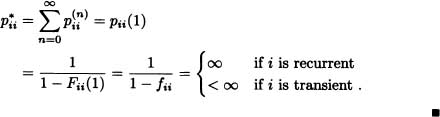
Corollary 9.3 Let i ![]() S. Then state i is recurrent if and only if
S. Then state i is recurrent if and only if ![]() or equivalently: i is transient if and only if
or equivalently: i is transient if and only if ![]() .
.
Proof:
Definition 9.30 A property of states is called a solidarity or class property, if whenever the state i has property i ↔ j, then the state j also has the property.
The following theorem proves that the recurrence, transience and period of a state are class properties.
Theorem 9.8 Suppose that i ↔ j. Then i is recurrent if and only if j is recurrent.
Proof: Since i ↔ j, there exist m, n ≥ 0 such that:
![]()
Assuming that i is recurrent, then
![]()
![]()
Therefore, if ![]() , then
, then ![]() .
. ![]()
Let {Xn; n ≥ 0} be a random walk in ![]() defined as
defined as
![]()
where Y1, Y2 . . . are independent and identically distributed random variables with:
P(Y1 = 1) = p and P(Y1 = −1) = 1 − p ≕ q with 0 < p < 1 .
It is clear that (Xn)n≥0 is a Markov chain with state space S = ![]() . For all i,j
. For all i,j ![]() S, we have that i ↔ j. Therefore, {Xn; n ≥ 0} is an irreducible Markov chain. Now
S, we have that i ↔ j. Therefore, {Xn; n ≥ 0} is an irreducible Markov chain. Now
![]()
Stirling’s formula (see Feller, 1968 Vol. I, page 52) shows that
![]()
where an ~ bn implies that ![]() . Using Stirling’s formula in the above expression for
. Using Stirling’s formula in the above expression for ![]() , obtain:
, obtain:
![]()
If we have p ≠ q, then 4pq < 1, and therefore ![]() , that is, if p ≠ q, the chain is transient. However, if p = q =
, that is, if p ≠ q, the chain is transient. However, if p = q = ![]() , then
, then ![]() , that is, if p = q =
, that is, if p = q = ![]() the chain is recurrent.
the chain is recurrent. ![]()
The following theorem proves that if the state j is transient, then the expected number of visits by the chain to the state j is finite, regardless of the state from which the chain has started.
Theorem 9.9 If j is transient, then ![]() for i
for i ![]() S.
S.
Proof: We know that
pij(s) − δij = Fij(s)pij(s)
![]()
since j is transient. Therefore, ![]() .
. ![]()
From the above theorem, it follows that, if j is transient, then:
![]()
The following question arises naturally: What happens to ![]() when state j is recurrent? To answer this question, we require the following concepts
when state j is recurrent? To answer this question, we require the following concepts
Definition 9.31 For i ![]() S, define:
S, define:
![]()
That is, μi represents the expected return time of the chain to state i given that the chain started from state i.
Definition 9.32 The recurrent state i is said to be positive recurrent if μi < ∞ and is said to be null recurrent if μi = ∞. It is clear from the definition of Fii(s) that:
![]()
Let us consider Example 9.28, with p = q = ![]() . In this case, it is known that:
. In this case, it is known that:
![]()
Therefore:
![]()
Thus,
![]()
and it follows that 0 is a null recurrent state. ![]()
Theorem 9.10 Let i ![]() S be a recurrent state with λ(i) = 1. Then:
S be a recurrent state with λ(i) = 1. Then:
![]()
Therefore, if i is null recurrent, then ![]() as n → ∞.
as n → ∞.
Proof: For the proof, the reader is refer to Resnick (1994). ![]()
It is to be observed that if i ![]() S is a null recurrent state with λ(i) = 1, then:
S is a null recurrent state with λ(i) = 1, then:
![]()
Theorem 9.11 If j → i and j is recurrent, then it satisfies:
1. fij = 1.
2. ![]() .
.
Proof:
1. Suppose that ![]() , with r being the least positive number with this property. We have:
, with r being the least positive number with this property. We have:
![]()
Therefore:
![]()
Which implies:
![]()
Since ![]() , it follows that fij = 1.
, it follows that fij = 1.
2. ![]() ; then
; then ![]() .
.
![]()
Theorem 9.12 Let {Xn;n ≥ 0} be an irreducible Markov chain whose states are recurrent and aperiodic. Then
![]()
independent of the initial state i.
Proof: For the proof, the reader is refer to Resnick (1994). ![]()
9.2.2 Measure of Stationary Probabilities
To complete the count of significant results in the context of the theory of Markov chains, we present the concept of invariant probability measure on the state space S and give a necessary and sufficient condition for the existence of such a measure.
Definition 9.33 Let {Xn;n ≥ 0} be a Markov chain with state space S. A probability measure π = (πh)h![]() s over S is called invariant or stationary if
s over S is called invariant or stationary if
for all j ![]() S. In other words, π is invariant if π = πP.
S. In other words, π is invariant if π = πP.
Theorem 9.13 Let {Xn;n ≥ 0} be an irreducible, aperiodic Markov chain with state space S. Then there exists an invariant probability measure over S if and only if the chain is positive recurrent. The determined probability measure is unique and satisfies the condition (9.6).
Without loss of generality we assume that S = ![]() .
.
Proof: Let us assume that there exists an invariant probability measure π over S that satisfies (9.6) since π = πP. Then π = πPn. That is:
![]()
If the states of a Markov chain are transient or null recurrent, then
![]()
and therefore πJ = 0 for all j, which is absurd, since ![]() . Suppose that the chain is positive recurrent and let:
. Suppose that the chain is positive recurrent and let:
![]()
1. Since the matrix Pn is stochastic:
![]()
Therefore, ![]()
On the hand, using the Chapman-Kolmogorov equation:
![]()
Then ![]() for all m. That is:
for all m. That is:
![]()
Suppose that for some j we have ![]() . Then
. Then
![]()
which contradicts the fact that j is recurrent. Therefore, for all j it satisfies:
![]()
That is, πP = π. Hence if πPn = π and
![]()
then for all ![]() > 0 there exists n0 ≥ 1 such that:
> 0 there exists n0 ≥ 1 such that:
![]()
Hence:
Since ![]() > 0 is arbitrary, (9.7) and (9.8) imply that
> 0 is arbitrary, (9.7) and (9.8) imply that
![]()
that is, ![]()
2. If it is assumed that there exists another stationary distribution (rk)k![]() s, then it is obtained similarly that:
s, then it is obtained similarly that:
![]()
Now taking the limit as n → ∞, we obtain:
![]()
![]()
Let {Xn;n ≥ 0} be a Markov chain with state space S = {1,2,3} and transition matrix
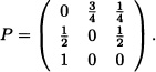
{Xn;n ≥ 0} is an irreducible, aperiodic Markov chain, and also S is finite so that the chain is positive recurrent. Thus, there exists a stationary probability measure π = (πj)j![]() s over S. Find these stationary probabilities πj.
s over S. Find these stationary probabilities πj.
Solution: Since πP = π, we obtain from the system:
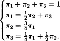
Solving the system, we obtain:
![]()
It is known that
![]()
for j = 1,2,3 independent of i; this implies, in particular, that the probability that, for some n sufficiently large, the chain is in state 1 given that it started from state i is equal to ![]() independent of the initial state i.
independent of the initial state i. ![]()
9.3 CONTINUOUS-TIME MARKOV CHAINS
In the previous section it was assumed that the time parameter t was discrete. This assumption may be appropriate in some cases, but in situations such as queueing models, the time parameter should be considered as continuous because the process evolves continuously over time. In probability theory, a continuous-time Markov process is a stochastic process {Xt;t ≥ 0} that satisfies the Markov property. It is the continuous-time adaptation of a Markov chain and hence it is called a continuous-time Markov chain (CTMC). In this section we are going to study the definition and basic properties of the CTMC with some examples.
Definition 9.34 Let X = {Xt;t ≥ 0} be a stochastic process with countable state space S. We say that the process is a continuous-time Markov chain if:
![]()
for all j, i, . . . , in−1 ![]() S and for all 0 ≤ t1 ≤ t < . . . < tn.
S and for all 0 ≤ t1 ≤ t < . . . < tn.
For Markov chains with discrete-time parameter we saw that the n-step transition matrix can be expressed in terms of the transition matrix raised to the power of n. In the continuous-time case there is no exact analog of the transition matrix P since there is no implicit unit of time. We will see in this section that there exists a matrix Q called the infinitesimal generator of the Markov chain which plays the role of P.
Definition 9.35 We say that the continuous-time Markov chain is homogeneous if and only if the probabilities P(Xt+s = j | Xs = i) is independent of s for all t.
Definition 9.36 The probability
pij(t) = P(Xt+s = j | Xs = i)
where s,t ≥ 0 is called the transition probability for the continuous-time Markov chain.
Let pij(t) be the probability of transition from state i to state j in an interval of length t. We denote:
P(t) = (Pij(t)) for all i, j ![]() S.
S.
We say that P(t) is a transition probability matrix. It is easy to verify that it satisfies the following conditions:
- pij (0) = δij.
- limt→0+ pij(t) = δij.
- For any t ≥ 0, i,j
 S, 0 ≤ pij(t) ≤ 1 and
- For all i,j S, for any s, t ≥ 0:
The above equation is called a Chapman-Kolmogorov equation for continuoustime Markov chains.
1. From part 2 of the above observation we get
![]()
where I is the identity matrix.
2. From part 4 of the above observation we get
that is, the family of transition matrices forms a semigroup.
Note 9.8 The following properties of transition probabilities are extremely important for applications of continuous-time Markov chains. They are outlined here without proof and the reader may refer to Resnick (1994).
1. Pij(t) is uniformly continuous on [0, ∞).
2. For each i ![]() S we have that
S we have that
![]()
exists (but may be equal to +∞).
3. For all i,j ![]() S with i ≠ j, we have that the following limit exists:
S with i ≠ j, we have that the following limit exists:
![]()

is called the infinitesimal generator of the Markov chain {Xt;t ≥ 0}.
Since P(0) = I, we conclude that:
Q = P′(0).
Note 9.9 Suppose that S is finite or countable. The matrix Q = (qij)i,j![]() s satisfies the following properties:
s satisfies the following properties:
1. qii ≤ 0 for all i.
2. qij ≥ 0 for all i ≠ j.
3. ![]() for all i.
for all i.
The infinitesimal generator Q of the Markov chain {Xt;t ≥ 0} plays an essential role in the theory of continuous-time Markov chains as will be shown in what follows.
1. A state i ![]() S is called an absorbing state if qi = 0.
S is called an absorbing state if qi = 0.
2. If qi < ∞ and ![]() , then the state i is called stable or regular.
, then the state i is called stable or regular.
3. A state i ![]() S is called an instantaneous state if qi = ∞.
S is called an instantaneous state if qi = ∞.
Theorem 9.14 Suppose that qi < ∞ for each i ![]() S. Then the transition probabilities pij(t) are differentiable for all t ≥ 0 and i,j
S. Then the transition probabilities pij(t) are differentiable for all t ≥ 0 and i,j ![]() S and satisfy the following equations:
S and satisfy the following equations:
1. (Kolmogorov forward equation)
![]()
2. (Kolmogorov backward equation)
![]()
or equivalently:
![]()
The initial condition for both the equations is P(0) = I.
Proof: For h > 0 and t ≥ 0 it is satisfied that:
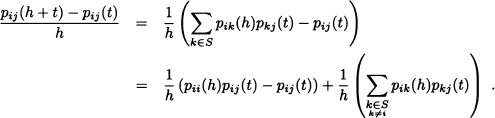
If h ↓ 0, then we have

where qii = −qi. ![]()
Formally the solution of the above equations can be cast in the form
![]()
If Q is a finite-dimensional matrix, the above series is convergent and has a unique solution for the system of equations. If Q is infinite dimensional we cannot say anything. Suppose that Q is a finite-dimensional matrix and diagonalizable and let β0, β1 . . . , βn be the distinct eigenvalues of the matrix Q. Then there exists a matrix A such that
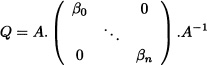
and in this case:

Note 9.10 For a given matrix Q we can define a stochastic matrix P as follows:
1. If qi ≠ 0,
2. If qi = 0, then Pij ≔ δij.
Let:
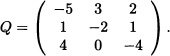
Then

Since
![]()
we have, for example:
![]()

Figure 9.8 State transition diagram for Example 9.32
Consider a two-unit system. Unit A has a failure rate λA and unit B has failure rate λB. There is one repairman and the repair rate of each of the units is μ. When both the machines fail, the system comes to a stop. In this case, {Xt; t ≥ 0} is a continuous-time Markov chain with state space S = {0, 1A, 1B, 2} where 0 denotes both the units have failed, 1A denotes unit A is working and unit B has failed, 1B denotes unit A has failed and unit B is working and 2 denotes both the units are working. The corresponding infinitesimal generator matrix is given by:
The state 0 is an absorbing state. The state transition diagram for this Markov chain is shown in Figure 9.8.
Then the transition probability matrix P is:
Definition 9.39 Let {Xt;t ≥ 0} be a continuos-time Markov chain with transition probability matrix (P(t))t≥0. A measure μ defined overr the state space S is called an invariant measure for {Xt;t ≥ 0} is called an invariant measure for {Xt;t ≥ 0} is and only if, for all t ≥0, μ satisfies
μ = μP(t)
that is, for each j ![]() S, μ satisfies:
S, μ satisfies:
![]()
If ![]() , then μ is called a stationary distribution.
, then μ is called a stationary distribution.
Let {Xt;t ≥ 0} be a continuous-time Markov chain with state space S = {0,1} and transition matrix given by:
![]()
It is easy to verify that ![]() is a stationary distribution for {Xt;t ≥ 0}.
is a stationary distribution for {Xt;t ≥ 0}. ![]()
Definition 9.40 Let {Xt;t ≥ 0} be a continuous-time Markov chain with infinitesimal generator Q and initial probability distribution λ on S. The discrete-time Markov chain with initial probability distribution λ and transition probability matrix P [given by (9.11)] is called the embedded Markov chain.
Now we will make use of the embedded Markov chain to give conditions that will guarantee the existence and uniqueness of a stationary distribution.
Theorem 9.15 Let {Xt;t ≥ 0} be a continuous-time Markov chain with infinitesimal matrix Q and let ![]() be the corresponding embedded Markov chain. If
be the corresponding embedded Markov chain. If ![]() is irreducible and positive recurrent with
is irreducible and positive recurrent with ![]() , then there exists a unique stationary distribution for {Xt;t ≥ 0}.
, then there exists a unique stationary distribution for {Xt;t ≥ 0}.
Proof: From the theory developed for discrete-time Markov chains, we have that the transition matrix PY of the embedded Markov chain ![]() has a unique stationary distribution υ with υPY = υ. The infinitesimal generator Q satisfies:
has a unique stationary distribution υ with υPY = υ. The infinitesimal generator Q satisfies:
Q = Λ(PY − IS).
Since Is is the identity matrix of order |S| and
Λ = diag(λi : i ![]() S)
S)
then μ ≔ υΛ −1 is a stationary measure for the process {Xt; t ≥ 0}. Because ![]() , by hypothesis, μ is finite. Let π = (πj : j
, by hypothesis, μ is finite. Let π = (πj : j ![]() S) be defined by
S) be defined by
![]()
or equivalently:
![]()
Thus we obtain a stationary distribution for {Xt; t ≥ 0} which is unique since υ is unique. In addition, from the relation between ![]() and {Xt; t ≥ 0} and from the way the invariant measure
and {Xt; t ≥ 0} and from the way the invariant measure ![]() was constructed, we conclude that:
was constructed, we conclude that:
![]()
![]()
![]() EXAMPLE 9.34 Birth-and-Death Processes
EXAMPLE 9.34 Birth-and-Death Processes
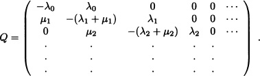
A birth-and-death process (BDP) is a continuous-time Markov chain {Xt,t ≥ 0} with state space S = ![]() such that the elements qi,i−1, qii and qi,i+1 of the intensity matrix Q are the only ones that can be different from zero. Let
such that the elements qi,i−1, qii and qi,i+1 of the intensity matrix Q are the only ones that can be different from zero. Let
λ ≔ qi,i+1 and μi ≔ qi,i−1
be the birth and death rates, respectively, as they are known. The matrix Q is given by:
It is clear that λih + o(h) represents the probability of a birth in the interval of infinitesimal length (t, t+h) given that Xt = i. Similarly μih+o(h) represents the probability of a death in the interval of infinitesimal length (t,t + h) given that Xt = i. From the Kolmogorov backward equations, we obtain:
![]()
Similarly, for the forward Kolmogorov equations, we obtain:
![]()
These equations can be solved explicitly for some special cases, as we will show later.
Next we will suppose that the state space S is finite and that λi > 0, μi > 0 for i ![]() S. The embedded Markov chain is irreducible and positive recurrent. Hence there exists a stationary distribution for {Xt; t ≥ 0}, say π = (π0, π1, . . ., πm). π is the solution of the system πQ = 0, which is given by:
S. The embedded Markov chain is irreducible and positive recurrent. Hence there exists a stationary distribution for {Xt; t ≥ 0}, say π = (π0, π1, . . ., πm). π is the solution of the system πQ = 0, which is given by:
![]()
Also ![]() . Then:
. Then:

![]() EXAMPLE 9.35 Linear Pure Death Process
EXAMPLE 9.35 Linear Pure Death Process
In the previous example of a birth-and-death process, suppose that λ0 = λ1 = . . . = 0 and that μi = iμ. Let us assume that the initial size of the population is N > 0. Then the backward and forward Kolmogorov equations are respectively
![]()
and
![]()
We obtain that
![]()
and therefore:
![]()
In other words, Xt has a binomial distribution with parameters N and e−μt. ![]()
Suppose that in the birth-and-death process we assume that μ1 = μ2 = . . . = 0 and λi = λ for all i ![]() S. Further we assume that X0 = 0 and pi(t) = P(Xt = i | X0 = 0). We obtain both Kolmogorov equations as follows:
S. Further we assume that X0 = 0 and pi(t) = P(Xt = i | X0 = 0). We obtain both Kolmogorov equations as follows:
![]()
By solving the above systems of equations, we obtain:
![]()
The random variable Xt has a Poisson distribution with parameter λt. The process {Xt;t ≥ 0} is called a Poisson process with parameter λ. ![]()
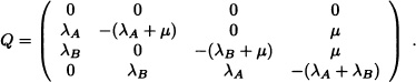
Assume that individuals remain healthy for an exponential time with mean ![]() before becoming sick. Assume also that it takes an exponential time to recover from sick to healthy again with mean sick time of
before becoming sick. Assume also that it takes an exponential time to recover from sick to healthy again with mean sick time of ![]() . If the individual starts healthy at time 0, then we are interested in tne probabilities of being sick and healthy in future times. Let state 0 denote the healthy state and state 1 denote the sick state.
. If the individual starts healthy at time 0, then we are interested in tne probabilities of being sick and healthy in future times. Let state 0 denote the healthy state and state 1 denote the sick state.
We have a birth-and-death process with
λ0 = λ, and μ1 = μ
and all other λi, μi are zero.
From the Kolmogorov backward equations, we have:


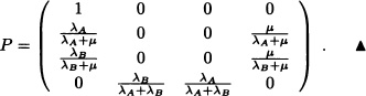
The stationary probability for the above equation is
![]()
and
![]()
9.4 POISSON PROCESS
In Example 9.36 of the previous section, we defined the Poisson process. This process, named after the French mathematician Simeon Denis Poisson (1781–1840), is one of the most widely used mathematical models. This process was also used by the Swedish mathematician Filip Lundberg (1876–1965) in 1903 in his doctoral thesis “Approximerad framställning af sannolikhetsfunktionen/ Återförsäkring af kollektivrisker” (Approximations of the probability function/ Reinsure of collective risks) to determine the ruin probability of an insurance company. Later the Swedish mathematician, actuary, and statistician Harald Cramer (1893–1985) and his pupils developed the ideas of Lundberg and constructed the so-called ruin process or Cramer-Lundberg model, which allows us to describe, at each instant, the reserve of an insurance company. Poisson processes have applications not only in risk theory but also in many other areas, for example, reliability theory and queueing theory.
Note 9.11 Let {Nt; t ≥ 0} be a Poisson process with parameter λ > 0. Then it satisfies the following conditions:
1. N0 = 0.
2. It has independent and stationary increments.
3. It has unit jumps, i.e.,
![]()
where Nh ≔ Nt+h − Nt.
The interested reader may refer to Hoel et al. (1972).
The examples for the Poisson processes are as follows:
- The number of particles emitted by a certain radioactive material undergoing radioactive decay during a certain period.
- The number of telephone calls originated in a given locality during a certain period.
- The occurrence of accidents at a given road over a certain period.
- The breakdowns of a machine over a certain period of time.

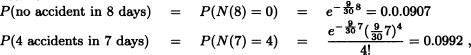
Suppose that accidents in Delhi roads involving Blueline buses obey a Poisson process with 9 accidents per month of 30 days. In a randomly chosen month of 30 days:
- What is the probability that there are exactly 4 accidents in the first 15 days?
- Given that exactly 4 accidents occurred in the first 15 days, what is the probability that all 4 occurred in the last 7 days out of these 15 days?
Solution: Let Nt ≔ “number of accidents in the time interval (0, t]” where the time t is measured in days.
Given that ![]() , the probability of exactly 4 accidents in the first 15 days is:
, the probability of exactly 4 accidents in the first 15 days is:
![]()
Now:
P(4 accidents occurred in last 7 days | 4 accidents occurred in 15 days)

Assume:
![]()
Suppose that incoming calls in a call center arrive according to a Poisson process with intensity of 30 calls per hour. What is the probability that no call is received in a 3-minute period? What is the probability that more than 5 calls are received in a 5-minute interval?
Solution: Let Nt ≔ “number of calls received in the time interval (0, t]” where the time t is measured in minutes.
From the data given above, it is known that ![]() . Therefore:
. Therefore:

Definition 9.41 Let {Nt;t ≥ 0} be a Poisson process with parameter λ > 0. If Tn is the time between the (n − 1)th and nth event, then {Tn; n = 1,2, . . .} are the interarrival times or holding times of Nt, and ![]() , n ≥ 1 is the arrival time of the nth event or the waiting time to the nth event.
, n ≥ 1 is the arrival time of the nth event or the waiting time to the nth event.
Theorem 9.16 The Ti’s have an exponential distribution with expected value ![]() .
.
Proof: Let T1 is the time of the first event. Then:
P(T1 > t) = P(Nt = 0) = e−λt.
Thus T1 has an exponential distribution with expected value ![]() . Now:
. Now:

Thus T2 also has an exponential distribution with expected value ![]() . Note also that T1 and T2 are independent and in general we have that the interarrival times Tn, n = 1,2, . . ., are independent and identically distributed random variables each with expected value
. Note also that T1 and T2 are independent and in general we have that the interarrival times Tn, n = 1,2, . . ., are independent and identically distributed random variables each with expected value ![]() .
. ![]()
Note 9.12 From the above theorem we have that Sn, the arrival time of the nth event, has a gamma(n, λ) distribution. Therefore the probability distribution function of Sn is given by:
![]()
Suppose that people immigrate into a territory at a Poisson rate λ = 1 per day.
- What is the expected time until the tenth immigrant arrives?
- What is the probability that the elapsed time between the tenth and the eleventh arrival exceeds two days?
Solution:
![]()
Suppose that exactly one event of a Poisson process occurs during the interval (0, t] Then the conditional distribution of T1 given that Nt = 1 is uniformly distributed over the interval (0, t] is:

Generally:
Theorem 9.17 Let Nt be a Poisson process with parameter λ. Then the joint conditional density of T1, T2, . . . , Tn given Nt = n is
![]()
Proof: Left as an exercise. ![]()
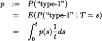
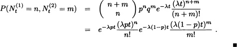
An application of the previous theorem is as follows: Consider a Poisson process {Nt; t ≥ 0} with intensity λ > 0. Suppose that if an event occurs, it is classified as a type-I event with probability p(s), where s is the time at which the event occurs, otherwise it is a type-II event with probability 1 − p(s). We now prove the following theorem.
Theorem 9.18 (Ross, 1996) If ![]() represents the number of type-i events that occur in the interval (0, t] with i = 1,2, then
represents the number of type-i events that occur in the interval (0, t] with i = 1,2, then ![]() and
and ![]() are independent Poisson random variables having parameters λp and λ(l−p), respectively, where:
are independent Poisson random variables having parameters λp and λ(l−p), respectively, where:
![]()
Proof: In the interval (0, t], let there be n type-I events and m type-II events, so that we have a total of n + m events in the interval (0, t]:

We consider an arbitrary event that occurred in the interval (0, t]. If it has occurred at time s, the probability that it would be a type-I event is p(s). In other words, we know that the time at which this event occurs is uniformly distributed in the interval (0, t]. Therefore, the probability that it will be a type-I event is
independently of other events. Hence ![]() is the probability of n successes and m failures in a Bernoulli experiment of n + m trails with probability of success p in each trial. We get
is the probability of n successes and m failures in a Bernoulli experiment of n + m trails with probability of success p in each trial. We get
If immigrants arrive to area A at a Poisson rate of ten per week and each immigrant is of English descent with probability ![]() , then what is the probability that no person of English descent will emigrate to area A during the month of February?
, then what is the probability that no person of English descent will emigrate to area A during the month of February?
Solution: By the previous proposition it follows that the number of Englishmen emigrating to area A during the month of February is Poisson distributed with mean ![]() . Hence the desired probability is
. Hence the desired probability is ![]() .
. ![]()
In the following algorithm, we simulate the sample path for the Poisson process using interarrival times which are i.i.d. exponentially distributed random variables.
Input: λ, T, where T is the maximum time unit.
Output: PP(k) for k = 0(1)T.
Initialization:
PP(0) ≔ 0.
Iteration:

where rand(0,1) is the uniform random number generated in the interval (0,1). Using the previous algorithm we obtain the sample path of Poisson process as shown in Figure 9.9 for λ = 2.5 and T = 10.
In the Poisson process, we assume that the intensity λ is a constant. If we assume a time-dependent intensity, that is, λ = λ(t), we get a nonhomogeneous Poisson process. More precisely, we have the following definition:
Definition 9.42 (Nonhomogeneous Poisson Process) A Markov process {Nt;, t ≥ 0} is a nonhomogeneous Poisson process with intensity function λ(t), t ≥ 0, if:
1. N0 = 0.
2. {Nt;t ≥ 0} has independent increments.
3. For 0 ≤ s ≤ t, the random variable Nt − Ns has a Poisson distribution with parameter ![]() . That is,
. That is,
![]()
for k = 0,1,2, . . ..

Figure 9.9 Sample path of Poisson process
![]()
is called the mean value function
Note 9.13 If {Nt;t ≥ 0} is a nonhomogeneous Poisson process with mean value function m(t), then {Nm−1(t);t ≥ 0} is a homogeneous Poisson process with intensity λ = 1. This follows since Nt is a Poisson random variable with mean m(t), and if we let Xt = Nm−1(t), then Xt is Poisson with mean m(m−1(t)) = t.
(Ross, 2007) John owns a cafeteria which is open from 8 AM. From 8 AM to 11 AM, the arrival rate of customers grows linearly from 5 customers per hour at 8 AM to 20 customers per hour at 11 AM. From 11 AM to 1 PM the arrival rate of customers is 20 customers per hour. From 1 PM to 5 PM the arrival rate of customers decreases linearly until it reaches a value of 12 customers per hour. If we assume that customers arrive at the cafeteria in nonoverlapping time intervals and are independent of each other, then:
- What is the probability that no customer arrives at the cafeteria between 8:30 AM and 9:30 AM?
- What is the expected number of customers in the same period of time?
Solution: Let Nt = “Number of customers arriving to the cafeteria in the time interval (0, t]”.
An adequate model for this situation is the nonhomogeneous Poisson process with intensity function λ(t) given by

and λ(t) = λ(9−t) for t < 9. Since ![]() where
where ![]() , then:
, then:
![]()
The expected number of clients in this period of time is 10. ![]()
Definition 9.44 (Compound Poisson Process) A stochastic process {Xt;t ≥ 0} is a compound Poisson process if
where {Nt; t ≥ 0} is a Poisson process and {Yi; i = 1,2, . . .} are independent and identically distributed random variables.
1. If Yt = 1, then Xt = Nt is a Poisson process.
2.

In life insurance, total claims are often modeled using a compound Poisson distribution. Claim numbers are usually assumed to occur according to a Poisson process and claim amounts have an appropriate density such as a log-normal or gamma. ![]()
Suppose that buses arrive at a sporting event in accordance with a Poisson process, and suppose that the numbers of customers in each bus are assumed to be independent and identically distributed. Then {Xt; t ≥ 0} is a compound Poisson process where Xt denotes the number of customers who have arrived by t. In equation (9.12), Yi represents the number of customers in the ith bus. ![]()
Suppose customers leave a supermarket in accordance with a Poisson process. If Yi, the amount spent by the ith customer, i = 1,2, …, are independent and identically distributed, then {Xt :t ≥ 0} is a compound Poisson process where Xt denotes the total amount of money spent by time t. ![]()
9.5 RENEWAL PROCESSES
The stochastic process {Nt; t ≥ 0} is called a counting process if Nt represents the number of events that have occurred up to time t.
In the previous section we dealt with the Poisson process, which is a counting process for which the periods of time between occurrences are i.i.d. random variables with exponential distribution. A possible generalization is to consider a counting process for which the periods of time between occurrences are i.i.d. random variables with arbitrary distribution. Such counting processes are known under the name renewal processes.
We have the following formal definition:
Definition 9.45 Let {Tn;n ≥ 1} be an i.i.d sequence of nonnegative random variables with common distribution F, where F (0) = P (Tn = 0) < 1.
The process {Sn; n ≥ 1} given by
![]()
is called a renewal process with duration or length-of-life distribution F.
If we interpret Tn as the period of time between the (n − l)th and the nth occurrence of a certain event, then the random variable Sn represents the nth holding time. Therefore, if we define the process {Nt : t ≥ 0} as
Nt := sup {n : Sn ≤ t}
then it is clear that Nt represents the number of events that have occurred (or renewals) up to time t.
From now on we will call, indistinctly, the processes {Sn; n ≥ 1} and {Nt; t ≥ 0} as renewal processes.
The well-known example of renewal processes is the repeated replacement of light bulbs. It is supposed that as soon as a light bulb burns out, it is instantaneously replaced by a new one. We assume that successively replaced bulbs are random variables having the same distribution function F. Let Sn = T1 + … + Tn, where Ti’s are the random life of the bulb with distribution function F. We have a renewal process {Nt; t ≥ 0} where Nt represents the number of bulbs replaced up to time t. ![]()
In the next theorem, we give a relation between the distributions of Nt and Sn.
Theorem 9.19 For k ![]()
![]() and t ≥ 0 we have that:
and t ≥ 0 we have that:
{Nt ≥ k;} if and only if {Sk ≤ t}.
Proof: It is clear that Nt ≥ k if and only if in the time interval [0, t] at least k renewals have occurred, which in turn occurs if and only if the kth renewal has occurred on or before t, that is, if (Sk ≤ t). ![]()
From the previous result, it follows for t ≥ 0 and k = 1,2, … that

where Fk denotes the kth convolution of F with itself.
Similarly, the expected number of renewals up to time t follows from the next expression:
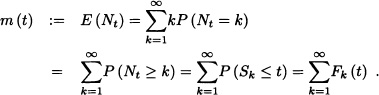
The function m(t) is called the mean value function or renewal function.
Consider {Tn; n = 1,2, …} with P(Tn = i) = p( 1 — p)i − 1 Here, Tn denotes the number of trials until the first success. Then Sn is the number of trials until the nth success:
![]()
The renewal process {Nt; t ≥ 0}, expressing the number of successes, is given by:
![]()
After simplification, we have
![]()
where [t] denotes the greatest integer function of t. ![]()
Consider a renewal process {Nt; t ≥ 0} with interarrival time distribution F. Suppose that the interarrival time has a uniform distribution between 0 and 1. Then the n-fold convolution of F is given by
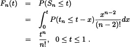
The renewal function for 0 ≤ t ≤ 1 is given by:
![]()
It can be shown that the renewal function m(t), 0 ≤ t ≤ ∞, uniquely determine the interarrival time distribution F.
In order to describe more accurately a renewal process we will introduce the following concepts:
Definition 9.46 For t > 0 define:
1. The age:
δt := t − SNt.
2. Residual lifetime or overshoot:
γt := SNt+1 − t.
3. Total lifetime:
βt := δt + γt.
For instance, consider the case of an individual who arrives, at time t, at a train station. Trains arrive at the station according to a renewal process {Nt; t ≤ 0}. In this case γt represents the waiting time of the individual at the station until the arrival of the train, δt the amount of time that has elapsed since the arrival of the last train and the arrival of the individual at the station and βt the total time elapsed between the train that the individual could not take and the arrival of the train that he is expected to take.
Definition 9.47 (Renewal Equation) Suppose {Nt; t ≥ 0} is a renewal process and T1 denotes the first renewal time. If T1 has density function f, then:

That is,
![]()
where F denotes the distribution function of T1. The above equation is known as the renewal equation. In the discrete case, the renewal equation is:
![]()
Consider the residual lifetime γt at time t. Let g(t) = E(γ(t)). Using the renewal equation, we can find g(t). Conditioning on T1 gives:
![]()
Now,
E (γ(t) | T1 = x > t) = x − t
while for T1 = x < t:
E (γ(t) | T1 = x < t) = g(t − x).
Hence,
![]()
is the renewal equation for g(t). ![]()
Consider a maintained system in which repair restores the system to as good as new condition and repair times are negligible in comparison to operating times. Let Ti, i = 1,2, …, represent the successive lifetimes of a system that, upon failure, is replaced by a new one or is overhauled to as-new condition. Let N(t) be the number of failures that have occurred up to time t, i.e., Nt = max{n : T1 + T2 + … + Tn ≤ t}.
The renewal function m(t) = E(Nt) is the expected number of failures that have occurred by time t. It satisfies the equation
![]()
Suppose Ti, i = 1, 2, …, follows exponential distribution with parameter λ so that ![]() . Then the renewal process {Nt; t ≥ 0} is a Poisson process with
. Then the renewal process {Nt; t ≥ 0} is a Poisson process with
![]()
and m(t) = λt. ![]()
Next we will discuss the asymptotic behavior of a renewal process. In the first place, we will see that, with probability 1, the total number of renewals, as the time tends to infinity, is infinity. As a matter of fact:
Theorem 9.20 For each renewal process {Nt : t ≥ 0} we have that:
![]()
Proof: For all n ≥ 1, we have

so that:
![]()
![]()
Theorem 9.21 With probability 1, we have
![]()
where μ := E(T1).
Proof: Since for any t > 0
![]()
then:
![]()
By using the strong law of large numbers, we have that:
![]()
Then:
![]()
![]()
Our next goal is to prove that the expected number of renewals per unit time tends to μ when t → ∞. We could think that this result is a consequence of the previous theorem. Unfortunately that is not true, since if Y, Y1, Y2, … are random variables such that Yn → Y with probability 1, we do not necessarily have that E(Yn) → E(Y).
Theorem 9.22 (The Elementary Renewal Theorem) Let {Nt; t ≥ 0} be a renewal process. Then:
![]()
![]()
It follows that:
![]()
Because SNt + 1 > t, we have (m(t) + 1) μ > E(t) = t, and we obtain that:
![]()
Since
SNt + 1 − t ≤ SNt + 1 − SNt = TNt + 1 ,
it follows that
![]()
If the random variables T1, T2, … are uniformly bounded, then there exists a number M > 0 such that
P(Tn ≤ M) = 1 .
Thus E (TNt + 1) ≤ M and we obtain
![]()
completing the proof in this case.
If the variables are not bounded, we can consider a fixed number K and construct the truncated process ![]() given by
given by
![]()
for n = 1,2, …. It is clear that ![]() . For the renewal process
. For the renewal process ![]() is determined by the process
is determined by the process ![]() and consequently we have:
and consequently we have:
![]()
Since
![]()
it follows that:
![]()
Allowing K → ∞ and using the monotone convergence theorem, it follows that:
![]()
![]()
Next, we will show that Nt has, asymptotically, a Gaussian distribution.
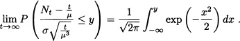
Theorem 9.23 Suppose μ = E(T1) and σ2 = V ar (T1) are finite. Then:

Proof: Fix x and let n → ∞ and t → ∞ so that:
![]()
Observing that T1, T2, … are i.i.d. random variables, the central limit theorem implies that:
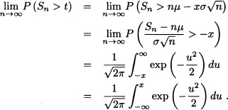
Since
![]()
we have

when t → ∞. Therefore

and it follow that:
Definition 9.48 A nonnegative random variable X is said to be a lattice if there exists d ≥ 0 such that:
![]()
That is, X is a lattice if it only takes on integral multiples of some nonnegative number d. The largest d having this property is called the period of X. If X is a lattice and F is the distribution function of X, then we say that F is a lattice.
(a) If ![]() , then X is a lattice with period 2.
, then X is a lattice with period 2.
(b) If ![]() , then X is a lattice with period 2π.
, then X is a lattice with period 2π.
(c) If ![]() , then X is not a lattice.
, then X is not a lattice.
(d) If X ![]() exp (λ), then X is not a lattice.
exp (λ), then X is not a lattice. ![]()
We will now state a result known as Blackwell’s theorem without proof. If F is not a lattice, then the expected number of renewals in an interval of length a from the origin is approximately ![]() . In the case of F being a lattice with period d, the Blackwell theorem asserts that the expected number of renewals up to nd tends to
. In the case of F being a lattice with period d, the Blackwell theorem asserts that the expected number of renewals up to nd tends to ![]() as n → ∞.
as n → ∞.
Theorem 9.24 Let {Nt; t ≥ 0} be a renewal process having renewal function m(t).
(a) If F is not a lattice, then
![]()
for a > 0 fixed.
(b) If F is a lattice with period d, then
![]()
where Rn is a random variable denoting the number of renewals up to nd.
The Blackwell theorem is equivalent to the following theorem, known as the key renewal theorem (Smith, 1953), and will be stated without proof.
Theorem 9.25 Let F be the distribution function of a positive random variable with mean μ. Suppose that h is a function defined on [0, ∞) such that:
(1) h(t) ≥ 0 for all t ≥ 0.
(2) h(t) is nonincreasing.
(3) ![]() h(t) dt < ∞
h(t) dt < ∞
and let Z be the solution of the renewal equation
![]()
Then:
(a) If F is not a lattice:
(b) If F is a lattice with period d, then for 0 ≤ c ≤ d we have that:

Next we are going to use the key renewal theorem to find the distributions of the random variables δt := t − SNt (age) and βt (total lifetime).
Theorem 9.26 For t ![]() (x, ∞) we have the function z(t) = P (δt > x) satisfying the equation
(x, ∞) we have the function z(t) = P (δt > x) satisfying the equation
![]()
so that, if μ < ∞, then:
![]()
Proof: Conditioning on the value of T1, we have for fixed x > 0:
![]()

we write:

Thus
![]()
so that the function h(t) := 1 − F (t + x) satisfies the key renewal theorem conditions, and as a consequence:
![]()
![]()
Theorem 9.27 The function g (t) = P (βt > x) satisfies the renewal equation
![]()
where t ⋁ x := max (t, x). Consequently,
![]()
if μ < ∞
Proof: Since
![]()
and

we have that:
![]()
Applying the key renewal theorem with h(t) = 1 − F(t ⋁ x) we obtain:
![]()
![]()
9.6 SEMI-MARKOV PROCESS
In this section, we give a brief account of the semi-Markov process (SMP) and the Markov regenerative process (MRGP). Knowledge of these concepts are required for building queueing models, introduced in the next chapter.
Definition 9.49 (Semi-Markov Process) Let {Yn; n ![]()
![]() } be a stochastic process with state space S =
} be a stochastic process with state space S = ![]() and {Vn; n
and {Vn; n ![]()
![]() } a sequence of nonnegative random variables. Let
} a sequence of nonnegative random variables. Let

and
U(t) := max{n ≥ 1 : Un ≤ t}, t ≥ 0 .
The continuous-time stochastic process {Xt; t ≥ 0} defined by
Xt := YU(t), t ≥ 0 ,
is called a semi-Markov process if the following properties hold:
(a) For all n ≥ 0:
![]()
(b)
![]()
The semi-Markov process {Xt; t ≥ 0} is also known as a Markov renewal process.
Note 9.15 {Yn, n ![]()
![]() } is a homogeneous Markov chain with transition probabilities given by:
} is a homogeneous Markov chain with transition probabilities given by:
![]()
{Yn, n ![]()
![]() } is known as the embedded Markov chain of the semi-Markov process {Xt; t ≥ 0}.
} is known as the embedded Markov chain of the semi-Markov process {Xt; t ≥ 0}.
Definition 9.50 M(t) = (mij(t))i,j![]() s with
s with
mij(t) := P(Yn+1 = j, Vn+1 ≤ t | Yn = i)
is called the semi-Markov kernel.
Definition 9.51 Let {Xt; t ≥ 0} be a semi-Markov process. Then:
1. The sojourn time distribution for the state i defined as:
![]()
2. The mean sojourn time in state i is defined as:

3.
Fij(t) = P(Vn+1 ≤ t | Yn = i, Yn+1 = j)
Note 9.16 For i, j ![]() S, we have:
S, we have:
![]()
Note 9.17 A continuous-time Markov chain is a semi-Markov process with:
![]()
Therefore:

Consider a stochastic process {Xt; t ≥ 0} with state space S = {1,2,3,4}. Assume that the time spent in states 1 and 2 follow exponential distributions with parameter λ1 = 2 and λ2 = 3, respectively. Further, assume that the time spent in states 3 and 4 follow general distributions with distribution function H3(t) and H4(t) (sojourn time distribution) respectively and are given by:

From Definition 9.49, {Xt,; t ≥ 0} is a semi-Markov process with state space S. ![]()
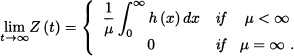
The following theorem describes the limiting behaviour of SMPs (see Cinlar, 1975).
Theorem 9.28 Let {Xt; t ≥ 0} be a SMP with {Yn; n ![]()
![]() } its embedded Markov chain. Suppose that {Yn; n
} its embedded Markov chain. Suppose that {Yn; n ![]()
![]() } is irreducible, aperiodic and positive recurrent. Then
} is irreducible, aperiodic and positive recurrent. Then
where μj is the mean sojourn time in state j and (πj)j![]() S is the stationary distribution of {Yn; n
S is the stationary distribution of {Yn; n ![]()
![]() }.
}.
Consider Example 9.53. Find the steady-state distribution of {Xt; t ≥ 0}.
Solution: {Xt; t ≥ 0} is a SMP with state space S = {1,2,3,4}. {Yn; n ![]()
![]() } is a homogeneous Markov chain with transition probability matrix
} is a homogeneous Markov chain with transition probability matrix

Since {Yn; n ![]()
![]() } is irreducible, aperiodic and positive recurrent, the stationary distribution π = (πi)i
} is irreducible, aperiodic and positive recurrent, the stationary distribution π = (πi)i![]() S exists and is obtained by solving
S exists and is obtained by solving
![]()
to get
![]()

Figure 9.10 State transition diagram for Example 9.55
The mean sojourn times for states i = 1,2,3,4 are given by:
![]()
Using equation (9.13), the steady-state probabilities for the SMP are given by:
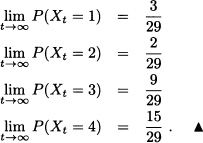
Consider a system with two components. Each component can fail with failure time exponentially distributed with parameter λ. The system has one repair unit and the repair time is constant with time T. Note that when both the components fail the system will be completely down. Assume that both the components can be repaired simultaneously and the repair time for both the components is a constant T. Let Xt denote the number of components working at time t. Figure 9.10 shows the state transition diagram for this model.
From Definition 9.49, we conclude that {Xt; t ≥ 0} is a semi-Markov process. Now:

By using the steps in Theorem 9.28, the steady state probabilities can be obtained. ![]()
Definition 9.52 (Markov Regenerative Process) Let {Yn; n ![]()
![]() } be a stochastic process with state space S =
} be a stochastic process with state space S = ![]() and {Vn; n
and {Vn; n ![]()
![]() } a sequence of nonnegative random variables. Let
} a sequence of nonnegative random variables. Let

and
U(t) := max{n ≥ 1 : Un ≤ t}, t ≥ 0 ,
The process {Xt; t ≥ 0} given by
Xt := YU(t), t ≥ 0 ,
is called a Markov regenerative process if:
(a) There exists S′ ⊂ S such that {Yn; n ![]()
![]() } is a homogeneous Markov chain with state space S′.
} is a homogeneous Markov chain with state space S′.
(b) For all n ≥ 0:

(c) ![]()
Note 9.18 {Yn; n ![]()
![]() } is a homogeneous Markov chain with state space S′ . Its transition probabilities are given by:
} is a homogeneous Markov chain with state space S′ . Its transition probabilities are given by:
![]()
Definition 9.53 K(t) = (kij(t))i,j![]() S′ with
S′ with
kij(t) := P(Y1 = j, V1 ≤ t | Y0 = i)
is called the global kernel of MRGP.
eij(t) := P(Y1 = j, V1 > t | Y0 = i)
is called the local kernel of MRGP. The matrix E(t) describes the behavior of the MRGP between two regeneration epochs of the embedded Markov chain {Yn, n ![]()
![]() }.
}.

Figure 9.11 State transition diagram for Example 9.56
Definition 9.55 Let {Xt; t ≥ 0} be a Markov regenerative process. Then:
1. The sojourn time distribution for state i is defined as:
![]()
2. The mean sojourn time in state j ![]() S between two successive regeneration epochs given that it started in state i
S between two successive regeneration epochs given that it started in state i ![]() S′ after the last regeneration is defined as:
S′ after the last regeneration is defined as:

3. The mean sojourn time in state j ![]() S between two successive regeneration epochs is defined as:
S between two successive regeneration epochs is defined as:
The following theorem describes the limiting behavior of MRGPs (see Cinlar, 1975).
Theorem 9.29 Let {Xt; t ≥ 0} be a MRGP with state space S and {Yn; n ![]()
![]() } its embedded Markov chain with state space S′ ⊂ S. Suppose that {Yn; n
} its embedded Markov chain with state space S′ ⊂ S. Suppose that {Yn; n ![]()
![]() } is irreducible, aperiodic and positive recurrent. Then
} is irreducible, aperiodic and positive recurrent. Then
where (πk)k![]() S′ is the stationary distribution of {Yn; n
S′ is the stationary distribution of {Yn; n ![]()
![]() }, μk is defined in equation (9.15) and αk,j is defined in equation (9.14).
}, μk is defined in equation (9.15) and αk,j is defined in equation (9.14).
Markov regenerative processes have wide applications in queueing models which are presented in the next chapter.

Figure 9.12 Relationship between various stochastic processes
Consider Example 9.55. Assume that when both the components fail, they cannot be repaired simultaneously. Assume that repair time is constant with time T. Let Xt denote the number of components working at time t. Figure 9.11 shows the state transition diagram for this model.
Based on the transition of the system moving from one state to other states, we conclude that {Xt; t ≥ 0} is a regenerative process. By using the steps in Theorem 9.29, the steady state probabilities can be obtained. ![]()
To conclude this chapter, we present Figure 9.12 to indicate the relationship of inclusion and exclusion among various important stochastic processes. For more details, readers may refer to Grimmett and Stirzaker (2001), Karlin and Taylor (1975), Medhi (1994), Lawler (2006), Resnick (1994), Ross (1996), and Ross (2007).
EXERCISES
9.1 Let Xt = A cos(ηt + ![]() ) be a cosine process, where A, η are real-valued random variables and
) be a cosine process, where A, η are real-valued random variables and ![]() is uniformly distributed over (0,2π) and is independent of A and η.
is uniformly distributed over (0,2π) and is independent of A and η.
a) Compute the covariance function of the process {Xt; t ![]()
![]() }.
}.
b) Is {Xt; t ![]()
![]() } covariance stationary.
} covariance stationary.
9.2 Consider the process Xt = A cos(wt) + B sin(wt) where A and B are uncorrelated random variables with mean 0 and variance 1 and w is a positive constant. Is {Xt; t ≥ 0} covariance/wide-sense stationary?
9.3 Show that an i.i.d. sequence of continuous random variables with common density function f is strictly stationary.
9.4 Show that a stochastic process with independent increments has the Markov property.
9.5 Suppose that a taxi continuously moves between the airport and two hotels according to a Markov chain with a transition probability matrix given by:

a) Argue that this Markov chain has a stationary distribution.
b) In the long run, what proportion of time will the taxi be in each of the three locations?
c) Suppose that you are at the airport and just about to get into this taxi when a very rude person barges ahead of you and steals the cab. If each transition that the taxi makes takes 25 minutes, how long do you expect to have to wait at the airport until the taxi returns?
9.6 One way of spreading information on a network uses a rumor-spreading paradigm. Suppose that there are 5 hosts currently on the network. Initially, one host begins with a message. In every round, each host that has the message contacts another host chosen independently and uniformly at random from the other 4 hosts and sends the message to that host. The process stops when all hosts have the message.
a) Model this process as a discrete-time Markov chain.
b) Find the transition probability matrix for the chain.
c) Classify the states of the chain as transient, recurrent or null recurrent.
9.7 Consider a Markov chain with state space {0,1,2,3,4} and transition matrix

a) Classify the states of the chain.
b) Determine the stationary distribution for states 1 and 2.
c) For the transient states, calculate μij, the expected number of visits to transient state j, given that the process started in transient state i.
d) Find P(X5 = 2 | X3 = 1).
9.8 The transition probability matrix of a discrete-time Markov chain {Xn; n = 1,2, … } having three states 1, 2 and 3 is

and the initial distribution is
π = (0.7, 0.2, 0.1).
Find:
a) P(X2 = 3) .
b) P(X3 = 2, X2 = 3, X1 = 3, X0 = 2) .
9.9 Consider a DTMC model which arises in an insurance problem. To compute insurance or pension premiums for professional diseases such as silicosis, we need to compute the average degree of disability at preassigned time periods. Suppose that we retain m degrees of disability S1, S2, … , Sm. Assume that an insurance policy holder can go from degree Si to degree Sj with a probability pij. This strong assumption leads to the construction of the DTMC model in which P = [pij] is the one-step transition probability matrix related to the degree of disability. Using real observations recorded in India, we considered the following transition matrix P:

a) Classify the states of the chain as transient, positive recurrent or null recurrent along each period.
b) Find the limiting distribution for the degree of disability.
9.10 Let p00 = 1 and, for j > 0, Pjj = p, Pj,j−1 = q where p + q = 1, define the transition probability matrix of DTMC.
a) Find![]() , the probability that absorption takes place exactly at the nth step given that the initial state is j.
, the probability that absorption takes place exactly at the nth step given that the initial state is j.
b) Find the expectation of this distribution.
9.11 Assume a DTMC {Xn; n = 1,2, … } with state space E = {0,1,2} and transition probability matrix P given by:
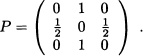
a) Classify the states of the Markov chain.
b)Find the distribution of Xn given that the initial probability vector is ![]() .
.
c) Examine whether there exists a limiting distribution for this Markov chain.
9.12 Consider a time homogeneous discrete-time Markov chain with transition probability matrix P and states {0,1,2,3,4} where:

a) Classify the states of the Markov chain as positive recurrent, null recurrent or transient.
b) Discuss the behavior of ![]() as n → ∞ for all i, j = 0,1, …, 4.
as n → ∞ for all i, j = 0,1, …, 4.
9.13 Consider a DTMC with states {0,1,2,3,4}. Suppose p0,4 = 1 and suppose that when the chain is in state i, i > 0, the next state is equally likely to be any of the states 0,1, …, i − 1.
a) Discuss the nature of the states of this Markov chain.
b) Discuss whether there exists a limiting distribution and find it if it exists.
9.14 A factory has two machines and one repair crew. Assume that probability of any one machine breaking down on a given day is α. Assume that if the repair crew is working on a machine, the probability that they will complete the repairs in one more day is β. For simplicity, ignore the probability of a repair completion or a breakdown taking place except at the end of a day. Let Xn be the number of machines in operation at the end of the nth day. Assume that the behavior of Xn can be modeled as a DTMC.
a) Find the transition probability matrix for the chain.
b) If the system starts out with both machines operating, what is the probability that both will be in operation two days later?
9.15 Consider a gambler who at each play of the game has probability p of winning one unit and probability q = 1 – p of losing one unit. Assume that successive plays of the game are independent. Suppose the gambler’s fortune is presently i, and suppose that we know that the gambler’s fortune will eventually reach N (before it goes to 0). Given this information, show that the probability he wins the next game is:

9.16 Consider a DTMC on the nonnegative integers such that, starting from i, the chain goes to state i + 1 with probability p, 0 < p < 1, and goes to state 0 with probability 1 – p.
a) Show that this DTMC is irreducible and recurrent.
b) Show that this DTMC has a unique steady state distribution π and find π.
9.17 Suppose a virus can exist in 3 different strains and in each generation it either stays the same or, with probability p, mutates to another strain, which is chosen at random. What is the probability that the strain in the nth generation is the same as that in the 0th?
9.18 There are two drive-through service windows at a very busy restaurant, in series, served by a single line. When there is a backlog of waiting cars, two cars begin service simultaneously. Out of the two cars being served, the front customer can leave if he finishes service before the rear customer, but the rear customer has to wait until the first customer finishes service. Consequently, each service window will sometimes be idle if their customer completes service before the customer at the other window. Assume there is an infinite backlog of waiting cars and that service requirements of the cars (measured in seconds) are exponential random variables with a mean of 120 seconds. Draw the state transition diagram that describes whether each service window is busy. What is the stationary probability that both service windows are busy?
9.19 Consider a taxi station where taxis and customers arrive independently in accordance with Poisson processes with respective rates of one and two per minute. A taxi will wait no matter how many other taxis are in the system. However, an arriving customer that does not find a taxi waiting leaves. Note that a taxi can accommodate only one customer. Let {Xt; t ≥ 0} denote the number of taxis waiting for customers at time t.
a) Draw the state transition diagram for this process.
b) Find the average time a taxi waits in the system.
c) Find the proportion of arriving customers that get taxis.
9.20 A particle starting at position A makes a random to-and-from motion in a circle over A, B, C, D, A such that if it reaches a position I(= A, B, C or D) at any step, in the next step, either it stays in the same position with probability ![]() or else jumps to the right (clockwise) or left (anticlockwise) with probability
or else jumps to the right (clockwise) or left (anticlockwise) with probability ![]() or
or ![]() respectively.
respectively.
a) Draw the state transition diagram for the process.
b) Determine the probability that the process will never return to state A having started at A initially. Give justification.
c) Find the limiting distribution for the process.
9.21 Customers arrive at a bank at a Poisson rate λ. Suppose two customers arrive in the first hour. What’s the probability that:
a) Both arrived in the first 20 minutes?
b) At least one arrived in the first 20 minutes?
9.22 An insurance company pays out claims on its life insurance policies in accordance with a Poisson process having rate λ = 5 per week. If the amount of money paid on each policy is exponentially distributed with mean $2000, what is the mean and variance of the amount paid by the insurance company in a four-week span?
9.23 Show that if N1(t) and N2(t) are independent Poisson processes with rate λ1 and λ2, respectively, then Nt = N1(t) + N2(t) is a Poisson process with rate λ1 + λ2.
9.24 Let {Nt; t ≥ 0} be a Poisson process with intensity parameter λ. Suppose each arrival is “registered” or recorded with probability p, independent of other arrivals. Let Mt be the counting process of registered or recorded events. Show that Mt is a Poisson process with parameter λp.
9.25 Consider the IIT Delhi Open House program. Assume that students from various schools arrive at the reception at the instants of a Poisson process with rate 2 per minute. At the reception main door, two program representatives separately explain the program to students entering the hall. Each explanation takes a time (in minutes) which is assumed to be exponentially distributed with parameter 1 and is independent of other explanations. After the explanation, the students enter the hall. If both representatives are busy the student goes directly into the hall. Let Xt be the number of busy representatives at time t. Without loss of generality, assume that the system is modeled as a birth-and-death process.
a) Write the generator matrix Q.
b) Write the forward Kolmogorov equations for the birth-and-death process {Xt; t ≥ 0}.
c) Derive the stationary distribution of the process.
9.26 Consider the New Delhi International Airport. Suppose that it has three runways. Airplanes have been found to arrive at the rate of 20 per hour. It is estimated that each landing takes 3 minutes. Assume a Poisson process for arrivals and an exponential distribution for landing times. Without loss of generality, assume that the system is modeled as a birth-and-death process.
a) What is the steady state probability that there is no waiting time to land?
b) What is the expected number of airplanes waiting to land?
c) Find the expected waiting time to land?
9.27 A cable car starts off with n riders. The times between successive stops of the car are independent exponential random variables, each with rate λ. At each stop, one rider gets off. This takes no time and no additional riders get on. Let Xt denote the number of riders present in the car at time t.
a) Write down the Kolmogorov forward equations for the process {Xt;t ≥ 0}.
b) Find the mean and variance of the number of riders present in the car at any time t.
9.28 Let {Xt; t ≥ 0} be a pure birth process with λn = nλ, n = 1,2,…, λ0 = λ; μn = 0, n = 1,2,….
a) Find the conditional probability that Xt = n given that X0 = i (1 ≤ i ≤ n).
b) Find the mean of this conditional distribution.
9.29 Suppose that an office receives two different types of inquiry: persons who walk in off the street and persons who call by telephone. Suppose the two types of arrival are described by independent Poisson processes with rate α1 and α2 for walk-in and the callers, respectively. What is the distribution of the number of telephone calls received before the first walk-in customer.
9.30 An insurance company wishes to test the assumption that claims of a particular type arrive according to a Poisson process model. The times of arrival of the next 20 incoming claims of this type are to be recorded, giving a sequence T1, … , T20.
a) Give reasons why tests for the goodness of fit should be based on the interarrival times Xi = Ti − Ti −1 rather than on the arrival times Ti.
b) Write down the distribution of the interarrival times if the Poisson process model is correct and state one statistical test which could be applied to determine whether this distribution is realized in practice.
c) State the relationship between successive values of the interarrival times if the Poisson process model is correct and state one method which could be applied to determine whether this relationship holds in practice.
9.31 Let us consider that the buses arrive at a particular stop according to a Poisson process with rate 10 per hour. A student starts waiting at the stop at 1:00.
a) What is the probability that no buses arrive in the next half-hour?
b) How many buses are expected to arrive in 2 hours?
c) What is the variance of the number of buses that arrive over a 5-hour period?
d) What is the probability that no buses arrive in the next half-hour given that one hasn’t arrived for over 2 hours?
e) If you wait until 2 o’clock and no buses have arrived, what is the probability that a student still has to wait at least a further half-hour before one comes?
9.32 According to an interest rate model which operates in continuous time, the interest rate rt may change only by upward jumps of fixed size ju or by downward jumps of fixed size jd (where jd < 0), occurring independently according to Poisson processes Nu(t) (with rate λu) and Nd(t) (with rate λd).

Figure 9.13 State transition diagram for Exercise 9.33
Let Tu denote the time of the first up jump in the interest rate, Td the time of the first down jump, T = min(Tu, Td) the time of the first jump. Further, let I be defined as an indicator taking the value 1 if the first jump is an up jump or 0 otherwise.
a) Determine expressions for the probabilities P{Tu > t}, P{Td > t} and P{T > t}.
b) Determine the distribution of I.
c) Show, by evaluating P{T > t and 1 = 1}, that I and T are independent random variables.
d) Calculate the expectation and variance of the interest rate at time t given the current rate r0. Hint: rt = r0 + juNu(t) + jdNd(t)
e) Show that {rt; t > 0} is a process with stationary and independent increments.
9.33 Consider Example 9.32. Assume that both units have a failure rate λ. The state transition diagram is shown in Figure 9.13.
a) Write the forward Kolmogorov equations for this system.
b) Determine the reliability of the system.
9.34 Consider an n-unit system in which 1 unit is active and the other n − 1 units are inactive. There is one repairman and the repair rate of each unit is α. The failure and repair rates are λ and μ, respectively. This system can be modeled as a birth-and-death process {Xt;t ≥ 0}. The state of the system is the number of working components. Determine the steady state probabilities of the states of the underlying system.
9.35 Consider a service station with two identical computers and two technicians. Assume that when both computers are in good condition, most of the work load is on one computer, exposed to a failure rate λ = 1, while the other computer’s failure rate is λ = 0.5. Further assume that, if one of the computer fails, the other one takes the full load, thus exposed to a failure rate λ = 2. Among the technicians, one is with repair rate μ = 2 while the second is with repair rate μ = 1. If both work simultaneously on the same computer, the total repair rate is μ = 2.5. Note that, at any given moment, they work so that their repair rate is maximized.
a) Determine the infinitesimal generator matrix Q.
b) Draw the state transition diagram of the system.
c) Determine the steady state probabilities and the system availability.
9.36 Consider a service station with two computers and a technician. Suppose that computer A fails on the average once per hour and computer B twice per hour. The technician can repair a computer in 3 minutes on average.
a) Determine the infinitesimal generator matrix Q.
b) Draw the state transition diagram of the system.
c) Determine the steady state probabilities and the system availability.
9.37 The occurrences of successive failures can be described by a Poisson process with mean time between arrivals of 50 minutes.
a) What is the probability that exactly 3 failures occur in the first 1000 minutes?
b) Find the probability of no failure in the first 500 minutes.
c) What is the probability that the first failure occurs after 400 minutes?
d) Compute the probability that the 4th failure occurs after 2000 minutes?
9.38 Consider an n-unit parallel redundant system. The system is operates when at least one of the n units is operating. Then the system fails when all units are down simultaneously. It will begin to operate again immediately by replacing all failed units with new ones. Assume that each unit operates independently. Also assume that each unit has an identical failure distribution which follows exponential distribution with parameter λ. Obtain the renewal function.
9.39 Consider Example 9.34. Suppose that Markov chain {Xt;t ≥ 0} with state space S is irreducible and positive recurrent. Determine the stationary distribution.
__________