CHAPTER 10

INTRODUCTION TO QUEUEING MODELS

10.1   INTRODUCTION

The queueing theory is considered to be a branch of applied probability theory and is often used to describe the more specialized mathematical models for waiting lines or queues. The concept of queueing theory has been developed largely in the context of telephone traffic engineering originated by A. K. Erlang in 1909. Queueing models find applications in a wide variety of situations that may be encountered in health care, engineering, and operations research (Gross and Harris, 1998). In this chapter, the reader is introduced to the fundamental concepts of queueing theory and some of the basic queueing models which are useful in day-to-day real life. Important performance measures such as queue length, waiting time and loss probability are studied for some queueing models.

Queueing systems are comprised of customer(s) waiting for service and server(s) who serve the customer. They are frequently observed in some areas of day-to-day life, for example:

1. People waiting at the check-in counter of an airport
2. Aeroplanes arriving in an airport for landing
3. Online train ticket reservation system
4. People waiting to be served at a buffet
5. Customers waiting at a barber shop for a hair cut
6. Sequence of emails awaiting processing in a mail server     

Certain factors which affect the performance of queueing systems are as follows:

1. Arrival pattern
2. Service pattern
3. Number of servers
4. Maximum system capacity
5. Population size
6. Queue discipline

To incorporate these features, David G. Kendall introduced a queueing notation A/B/C/X/Y/Z in 1953 where:

A   is the interarrival time distribution

B   is the service time distribution

C   is the number of servers

X   is the system capacity

Y   is the population size

Z   is the queue discipline

The symbols traditionally used for some common probability distributions for A and B are given as:

D   Deterministic (constant)

E_k   Erlang-k

G   General service time

GI   General independent interarrival time

H_k   k-Stage hyperexponential

M   Exponential (Markovian)

PH   Phase type

In this chapter, an infinite customer population and service in the order of arrival [first-in first-out (FIFO)] are default assumptions. Hence, for example M/M/1/∞, where M stands for Markovian or memoryless. The first M denotes arrivals following a Poisson process, the second M denotes service time following exponential distribution, 1 refers to a single server and ∞ refers to infinite system capacity. Also there is an additional default assumption: interarrival and service times are independent. In a GI/D/c/N queueing model, GI denotes a general independent interarrival time distribution, D denotes a deterministic (constant) service time distribution, c denotes the number of servers and N refers to the number of waiting spaces including one in service.

Figure 10.1   M/M/1/∞ queueing system

The queueing systems in real life are quite complex as compared to the existing basic queueing models. As the real-life system complexity increases, it becomes more difficult to analyze the corresponding queueing system. A model should be made as simple as possible but at the same time it should be close to reality. In this chapter, we describe simple queueing models and analyze them by studying their desired characteristics. The real-world phenomenon can be popularly mapped to one of these queueing models.

10.2   MARKOVIAN SINGLE-SERVER MODELS

10.2.1   M/M/1/∞ Queueing System

Definition 10.1 (M/M/1/∞ Queueing System) The M/M/1/∞ or simply M/M/1 queueing system describes a queueing system with both interarrival and service times following exponential distribution with parameters and μ, respectively, one server, unlimited queue size with FIFO queueing discipline and unlimited customer population. It is shown in Figure 10.1 with arrival rate and service rate μ.

Theorem 10.1 Let X_t be a random variable denoting the number of customers in the M/M/1 queueing system at any time t. Define:

P_n(t) = P(X_t = n), n = 0,1, 2, · · · , t ≥ 0.

Let /μ = ρ. When ρ < 1, the steady state probabilities are given by:

P_n = P(X_t = n) = (1 − ρ)ρⁿ, n = 0,1, 2, · · · .

Proof:   The state transition diagram for the M/M/1 queueing system is shown in Figure 10.2. The stochastic process {X_t;t ≥ 0} in the M/M/1 queueing system can be modeled as a homogeneous continuous-time Markov chain (CTMC) (refer to Section 9.3). In particular, this system can be modeled by a birth-and-death process (BDP) with birth rates _n = , n = 0,1, · · ·, and death rates μ_n = μ, n = 1, 2, · · · . When ρ < 1, the underlying CTMC is irreducible and positive recurrent and has stationary distribution. Note that the stationary distribution holds good only for the system in equilibrium, which is attained asymptotically. Moreover, when the process attains equilibrium, its behavior becomes independent of time and its initial state. Hence, the steady state balance equations can be obtained as discussed in Section 9.4 and is given by:

Figure 10.2   State transition diagram for M/M/1/∞ queueing system

0   =   −P₀ + μP₁
0   =   P_n−1 − (+ μ)P_n + μP_n+1,    n = 1, 2, · · · .

Solving the above equations, we get

so that:

The value of P₀ can be computed by using the fact that the sum of all the probabilities must be equal to 1, i.e., Hence, when ρ < 1:

The steady state probabilities are given by:

Note 10.1 Equation (10.1) represents the probability mass function of a discrete random variable denoting the number of customers in the system in the long run. Clearly this distribution follows a geometric distribution with parameter I − ρ. Moreover, as t → ∞, the system state depends neither on t nor on the initial state. The sequence {P_n, n = 0,1, · · ·} is called the steady state or stationary distribution. Here, ρ < 1 is a necessary and sufficient condition for the steady state solution to exist; otherwise the size of the queue will increase without limit as time advances and therefore steady state solution will not exist.

Note 10.2  In case the arrivals follow a Poisson process, a customer arriving to the queue in the steady state sees exactly the same statistics of the number of customers in the system as for “real random times”. In a more condensed form, this is expressed as Poisson Arrivals See Time Averages, abbreviated PASTA (Wolff, (1982)). Since M/M/1 queueing system satisfies the PASTA property, an arriving customer finds n customers in the system with probability P_n.

Theorem 10.2 Let L_s be the average number of customers in the M/M/1 queueing system and L_q be the average number of customers in the queue. Then:

Proof:  Using (10.1), the mean number of customers can be found. Note that the number of customers in the system is the sum of the number of customers in the queue and the number of customers in service. Hence:

After simple calculations, we get:

As expected, these equations show that with increasing load, i.e., as ρ → 1, the mean number of customers in the system grows and the probability of an idle system decreases. Similarly, the average number of customers in the queue can be computed as:

Note 10.3  The probability that the server is busy is another performance measure of the queueing system. The probability that the server is busy when the system is in equilibrium is known as the utilization factor ρ. Clearly, this utilization factor for the M/M/1 queue is equal to 1 − P₀ = ρ, which is also the traffic intensity.

Note 10.4 The number of customers in the system is of importance from the management’s perspective and interest. Besides, the average queue size and average system size are also important parameters that represent the quality of service. Two more measures important from the customer’s point of view are the average time spent in the system (T_s) and the average time spent in the queue (T_q). One of the most significant contributions in queueing theory is Little’s formula, which gives the relation between the average number of customers in the system (L_s) and the average time spent in the system (T_s) and also between the average number of customers in the queue (L_q) and T_q:

It is justified that, using the average time spent in the system, T_s, the average number of the customers during this time is T_s, where is the average number of arrivals per unit time. It is very important to note that no assumption is made on the interarrival distribution, the service time distribution and the queue discipline. The first formal proof for Little’s result appeared in Little (1961). Usually the average waiting time of a customer is difficult to calculate directly. Relation (10.3) comes to our rescue, because the evaluation of mean number of customers in the system is relatively easy. As an example, it is derived for the M/M/1 queueing system from (10.2):

It can be deduced that:

Note 10.5 The variance of the four measures are given by (left as an exercise for the reader):

        Var(Number of customers in the system)   =   

         Var(Number of customers in the queue)   =   

Var (Waiting time of customers in the system)   =   

Var (Waiting time of customers in the queue)   =   

Theorem 10.3 Let W be the random variable which denotes the waiting time of a customer in the M/M/1 queueing system. Then, the distribution of waiting time is:

Proof:   An arriving customer has to wait only when there is one or more customer in the system. Hence the waiting time of the customer will be 0 if the system is empty. Thus, the probability of the event W = 0 is equivalent to the probability of the system being empty, i.e.:

P(W = 0) = P(system is empty) = 1 − ρ.

When the system is not empty, i.e., there is one or more customers in the system, say n, then the arriving customer has to wait until all the n customers get serviced. Note that as the service time follows exponential distribution with parameter μ, which has the memory less property, the residual (remaining) service time of the customer in service also follows exponential distribution with parameter μ. Hence, the waiting time of a customer who arrives when n customers are already in the system follows a gamma distribution with parameters n and μ. Thus:

We know that:

Substituting (10.7) and (10.8) in (10.6), we get:

Hence:

Similarly, we obtain the distribution of the total time spent by a customer in the system.

Theorem 10.4 Let T denote the random variable for the total time spent by a customer in the M/M/1 queueing system. Then the distribution of total time spent is given by:

P(0 < T < t) = 1 − e^{−μ(1−ρ)t}.

Proof:   As we evaluate the waiting time distribution, we have:

Note 10.6 This shows that T has an exponential distribution with parameter μ − . Hence, the average total time spent by a customer in the system is given by:

The above result is the same as that obtained in equation (10.4) using Little’s formula. It can also be verified that

EXAMPLE 10.1

Consider a unisex hair salon where customers are served on a first-come, first-served basis. The data show that customers arrive according to a Poisson process with a mean arrival rate of 5 customers per hour. Because of its excellent reputation, customers are always willing to wait. The data further show that the customer processing time is exponentially distributed with an average of 10 minutes per customer. This system can be modeled as a M/M/1 queueing system. Then, in the long run:

(a) What is the average number of customers in the shop?

(b) What is the average number of customers waiting for a haircut?

(c) What is the probability that an arrival can walk right in without having to wait at all?

Solution: Let X_t be the random variable denoting the number of customers in the salon at any time t. Then the system can be modeled as a M/M/1 queueing system with {X_t;t ≥ 0} as the underlying stochastic process. Here = 5 per hour and μ = 6 per hour. Hence, .

(a) The average number of customers in the shop:

(b) The average number of customers waiting for a haircut:

(c) The probability that an arrival can walk right in without having to wait at all:

P₀ = 1 − ρ = 0.1667 .     

EXAMPLE 10.2

Consider the New Delhi International Airport. Assume that it has one runway which is used for arrivals only. Airplanes have been found to arrive at a rate of 10 per hour. The time (in minutes) taken for an airplane to land is assumed to follow exponential distribution with mean 3 minutes. Assume that arrivals follow a Poisson process. Without loss of generality, assume that the system is modeled as a M/M/1 queueing system.

(a) What is the steady state probability that there is no waiting time to land?

(b) What is the expected number of airplanes waiting to land?

(c) Find the expected waiting time to land.

Solution: We model the given problem as a M/M/1 queueing system where each state represents the number of airplanes landing. The arrival rate is 10 per hour and the service rate is 20 per hour.

(a) The required probability that an airplane does not have to wait to land is:

P(runway is available) = P₀ = 1 − ρ = 0.5.

(b) From equation (10.3), the expected number of airplanes waiting to land is:

L_q = 0.5.

(c) Using Little’s formula, the expected waiting time to land is:

T_q = 0.05 hours.     

EXAMPLE 10.3

Consider the online ticket reservation system of Indian Railways. Assume that customers arrive according to a Poisson process at an average rate of 100 per hour. Also assume that the time taken for each reservation by a computer server follows an exponential distribution. Find out at what average rate the computer server should issue an e-ticket in order to ensure that a customer will not wait more than 45 seconds with a probability of 0.95.

Solution: P(W ≤ 45) = 0.95. Using equation (10.5), 1 − ρe^−45(μ−) = 0.95 where per second. From the stability condition, μ > = 0.02778. Simple calculations yield:

Solving, we get:

μ = 0.0508.

Hence, the server issues the e-ticket at an average 19.685 seconds in order to ensure that a customer does not wait more than 45 seconds.     

EXAMPLE 10.4

In a mobile handset manufacturing factory, components arrive according to a Poisson process with rate . Assume that the testing time of the components is exponential with mean 1/μ and there is one testing machine for the testing purpose. During the testing period, with probability p the product is considered to be faulty and sent back to the production unit queue.

(a) Determine the number of handsets in the queue of the production unit on average in the steady state.

(b) Find the average response time of a production unit in the steady state.

Solution: This system can be modeled as a M/M/1 queueing model with retrials. The state transition diagram for the underlying queueing model is shown in Figure 10.3.

The balance equations for this queueing model are:

P₀ = (1 − p)μP₁
( + (1 − p)μ)P_k = P_k−1 + (1 − p)μP_k+1, k = 1, 2, ··· .

Figure 10.3   State transition diagram

Figure 10.4   M/M/1/N queueing system

(a) The average number of customers in the queue is given by:

where

(b) The average response time is given by:

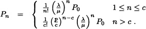
10.2.2   M/M/1/N Queueing System

We consider the single-server Markovian queueing system in which only a finite number of customers are allowed.

Definition 10.2 (M/M/1/N Queueing System) This system is a type of M/M/1/∞ queue with at most N customers allowed in the system. When there are N customers in the system, i.e., one customer is under service and the remaining N − 1 customers are waiting in the queue, new arriving customers are blocked. The state transition diagram for this system is shown in Figure 10.4.

Theorem 10.5 The state probabilities in equilibrium for the M/M/1/N queueing system are given by:

Proof:   Let X_t be a random variable denoting the number of customers in the system at any time t. For the M/M/1/N queueing system, {X_t;t ≥ 0} is a BDP with birth rates _n = , n = 0, 1, ···, N − 1, and death rates μ_n = μ, n = 1, 2, · · ·, N. Since the BDP {X_t;t ≥ 0} with finite state space S = {0,1, · · ·, N} is irreducible and positive recurrent, the equilibrium probabilities, denoted by (P_i)_iS, exist (refer to Example 9.34). Hence (P_i)_iS are given by:

with:

Substituting _n = , n = 0,1, · · ·, N − 1, and μ_n = μ, n = 1, 2, · · ·, N, in the above equations, we obtain the state probabilities in equilibrium.     

Note 10.7 The state probability P_N is called the blocking probability since the customers are blocked when the system is in state N. In this finite-state queueing model, the effective arrival rate is given as _eff = (1 − P_N).

Note 10.8 Using the state probabilities, one can compute the average number of customers in the system, which is given by:

Using Little’s formula, the average time spent by a customer in the system can be calculated as

where _eff is the effective arrival rate to the system.

The waiting time distribution for this M/M/1/N queueing system is left as an exercise for the reader.

EXAMPLE 10.5

Consider a message switching center in Vodafone. Assume that traffic arrives as a Poisson process with average rate of 180 messages per minute. The line has a transmission rate of 600 characters per second. Suppose that the message length discipline follows an exponential distribution with an average length of 176 characters. The arriving messages are buffered for transmission where buffer capacity is, say, N. What is the minimum N to guarantee that P_N < 0.005.

Solution: This system can be modeled as a M/M/1/N queueing system, where each state represents the number of messages in the switching center. In this example, = 3 × 176 = 528 characters per second and μ = 600 characters per second. Hence, ρ = = 0.88. From equation (10.9), the probability that all the buffers are filled is:

The above equation can be solved for P_N = 0.005 with ρ = 0.88 to obtain N = 26.     

EXAMPLE 10.6

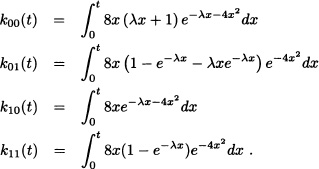
Consider a M/M/1/2 queueing system. Let P_n(t) be the probability that there are n customers in the system at time t given that there was no customers at time 0. Find the time-dependent probabilities P_n(t) for n = 0,1, 2.

Solution: The Kolmogorov forward equations for the M/M/1/2 queueing system are:

Taking the Laplace transform on both sides with the initial condition that the system begins in state 0, we obtain:

In matrix form

where:

For ≠ μ, the roots of det(A(s)) = 0 are:

Solving the above equations for (s), n = 0,1, 2, by using matrix inversion, we get:

Applying partial fraction techniques and then taking the inverse Laplace transform, for ≠ μ, we get:

EXAMPLE 10.7

A person repairing motor cars finds that the time spent on repairing a motor car follows an exponential distribution with mean 40 minutes. The shop can accommodate a maximum of 7 motor cars including the one under repair. The motor cars are repaired in the order in which they arrive, and the arrivals can be approximated by a Poisson process with an average rate of 15 per 10-hour day. What is the probability of the repair person being idle in the long run? Also, find the proportion of time the shop is not full in the long run.

Solution: This repair system can be modeled as a M/M/1/N queueing model where each state of the system represents the number of motor cars being repaired. Here and Hence, from equation (10.9), we get:

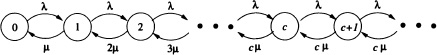
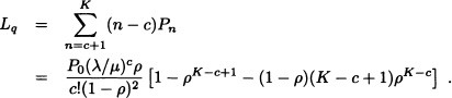
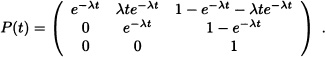
Figure 10.5   M/M/c/∞ queueing system

Further, the expected idle time of the repair person is P₀. The proportion of time that the shop is not full is:

Thus, the shop is not full 87.5% of the time in the long run.     

10.3   MARKOVIAN MULTISERVER MODELS

10.3.1   M/M/c/∞ Queueing System

We consider a multiserver queueing system M/M/c/∞. The state transition diagram for this system is shown in Figure 10.5. The corresponding steady state equations are given by:

0     =     P₀ − μP₁
0     =     P_n−1 − ( + nμ)P_n + (n + 1)μP_n+1, n = 1, 2, ···, c − 1
0     =     P_n−1 − ( + cμ)P_n + cμP_n+1, n = c, c + 1, ··· .

The steady state probabilities will exist for ρ < 1, where ρ = . Solving the above equations, we get the steady state probabilities

Using the fact that P_n = 1, we get:

Note 10.9 The probability that an arriving customer has to wait is given by

where P₀ is given by (10.11). This is known as the Erlang-C formula.

Note 10.10 The average number of customers in the queue is given by:

Using Little’s formula we evaluate T_q, T_s and L_s:

EXAMPLE 10.8

Consider Example 10.2. Further assume that it has three runways. In this scenario, assume that the arrival rate is 20 per hour and the service rate is 20 per hour. Without loss of generality, assume that the system is modeled as a M/M/3 queueing system.

(a) What is the steady state probability that there is no waiting time to land?

(b) What is the expected number of airplanes waiting to land?

(c) Find the expected waiting time to land.

Solution: We model the problem as a M/M/3 queueing system where each state represents the number of airplanes landing. The arrival rate is 20 per hour and the service rate is 20 per hour.

(a) The required probability that an airplane does not have to wait to land is

P(at least one runway is available)

=     P(Less than 3 airplanes are landing)
=     P₀ + P₁ + P₂

where P_i is the steady state probability of the system being in state i. Substituting the values of P_i using equations (10.10) and (10.11), the desired probability is 0.909.

(b) From equation (10.12), the expected number of airplanes waiting to land is:

(c) From equation (10.13), the expected waiting time to land is:

T_q = 0.0022725.     

EXAMPLE 10.9

Consider Walmart supermarket with 7 counters. Assume that 9 customers arrive on an average every 5 minutes while each cashier in the counter can serve on an average three customers in 5 minutes. Assume that arrivals follow a Poisson process and service times follow exponential distribution. Find:

(a) Average number of customers in the queue

(b) Average time a customer spends in the system

[c) Average number of customers in the system

(d) Optimal number of counters so that the proportion of time a customer has to wait is at most 10 seconds

Solution: This system is modeled as a M/M/7/∞ queueing system. Here, and The state probabilities are given by:

Using the fact we get P₀ = 0.0496.

(a) Average number of customers in the queue:

(b) Average time a customer spends in the system: T_s = 0.015694.

(c) Average number of the customers in the system: L_s = 3.02825.

(d) Using the fact that < 1, we get c > 3. Further, since it is required that T_q ≤ 10 seconds = 0.1667 minutes, by trial and error, we get that, for c = 4, T_q = 0.2121 and, for c = 5, T_q = 0.0786. Hence the optimal number of servers that must be installed in order that T_q < 10 seconds is c = 5.     

EXAMPLE 10.10

Suppose that Air India airlines is planning a new customer service center at London. Assume that each agent can serve a caller with an exponentially distributed service time with an average of 4 minutes. Also assume that calls arrive randomly as a Poisson process at an average rate of 30 calls per hour. Also assume that the system has a large message buffer system to hold calls that arrive when no agents are free. How many agents should be provided so that the average waiting time for those who must wait does not exceed 2 minutes?

Solution: This system can be modeled as a M/M/c/∞ queueing system where = and μ = . We require that for such a system to be stable, < 1 ⇒ c > 2. By trial and error, we obtain, for c = 3, T_q = 0.5925. Hence the number of agents who must be provided so that the average waiting time T_q < 2 is c = 3.     

EXAMPLE 10.11

A situation in which a customer refuses to enter a queueing system because the queue is too long is said to be balking. On the other hand, a customer who enters the system but leaves the queue after some time without receiving service because of excessive waiting time is said to be reneging. Assume that any customer who leaves the system and then decides to return after some time is a new arrival. Consider the M/M/c queueing system with the following:

1. (Balking) An arriving customer who finds that all the servers are busy may join the system with probability p or balk (does not join) with probability 1 − p.

2. (Reneging) A customer already in the queue may renege, i.e., leave the system without obtaining service. It is assumed that the time spent by such a customer in the system follows an exponential distribution with parameter β.

Find the steady state probability of the M/M/c system with:

(a) Only balking is possible.

(b) Only reneging is possible.

(c) Both balking and reneging are possible.

Solution:

(a) Consider the M/M/c with balking. Note that the arriving customer will enter the system if any server is not busy. This model can be viewed as a birth-and-death process with the arrival rate for the system being _n = , n = 0,1, ···, c − 1, _n = p, n = c, c + 1, · · · . The service rate is μ_n = nμ, n = 1, 2, ···, c, μ_n = c + 1, c + 2, · · · . The state transition diagram for this model is shown in Figure 10.6.

Figure 10.6   M/M/c queueing system with balking

Figure 10.7   M/M/c queueing system with reneging

The steady state probability is given as:

(b) Consider the M/M/c system with reneging. In this case, the customer will not leave the system when the customer is under service. Hence, the arrival rate is _n = , n = 0,1, · · · . But the service rate is μ_n = nμ, n = 1, 2, · · ·, c, μ_n = (n − c)β + c μ, n = c + 1, c + 2, ··· . The state transition diagram for this model is shown in Figure 10.7. Accordingly, the steady state probability is given as:

(c) Consider the M/M/c with both balking and reneging. In this case, the arrival rate is _n = , n = 0,1, · · ·, c − 1, _n = p, n = c, c + 1, · · · . The service rate is μ_n = nμ, n = 1, 2, · · ·, c, μ_n = (n − c)β + cμ, n = c + 1, c + 2, · · · . Hence, the steady state probability is given as

where P₀ is obtained from the fact that      

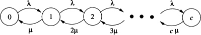
Figure 10.8   M/M/c/c/ loss system

10.3.2   M/M/c/c Loss System

This loss system is also known as the Erlang loss system. The state transition diagram for this loss system is shown in Figure 10.8. Solving the balance equations for steady state probabilities, we get

where

The above state probabilities indicate that the system state follows a truncated Poisson distribution with parameter ρ. The average number of customers in the system is given by:

Definition 10.3 (Erlang-B Formula) The blocking probability P_c is also called the Erlang-B formula and is given by:

Note 10.11 It is a fundamental result used for telephone traffic engineering problems and can be used to select the appropriate number of trunks (servers) needed to ensure a small proportion of lost calls (customers). Observe that the steady state distribution depends on the service time distribution only through its mean (since ρ = /μ). Hence, the Erlang-B formula also holds good for the M/G/c/c loss system where service time follows a general distribution. The important property of B(c,ρ) is illustrated in Figures 10.9 and 10.10. From Figure 10.9, for a fixed ρ, blocking probability, B(c,ρ) monotonically decreases to zero as the number of servers increases. From Figure 10.10, for a fixed number of servers c, the blocking probability B(c,ρ) monotonically increases to unity as ρ increases.

Figure 10.9   Erlang-B formula versus number of servers

Figure 10.10   Blocking probability versus ρ

EXAMPLE 10.12

A rural telephone switch has C circuits available to carry C calls. A new call is blocked if all circuits are busy. Suppose calls have duration (in minutes) which has exponential distribution with mean 1 and interarrival time (in minutes) of calls is also exponential with mean 1. Assume that calls arrive independently. Given that = 1 and μ = 1, so that Using Erlang-B formula given in (10.16), the probability that the system is blocked in the steady state is:

EXAMPLE 10.13

Suppose that Spencer supermarket in Chennai has decided to construct a parking system in the supermarket. An incoming four wheeler is not allowed inside the parking system when all the lots are in use. On average 100 four wheelers arrive to the system per hour following a Poisson process and the average time that the four wheeler spends in the parking lot is 4 minutes. Enough parking lots are to be provided to ensure that the probability of the system being full does not exceed 0. 005. How many lots should be constructed?

Solution: This system can be modeled as a M/G/c/c system with:

Using the Erlang-B formula in equation (10.16), we obtain the blocking probability

The smallest c such that P_B ≤ 0.005 is 14. Hence, we conclude that 14 lots are required.   

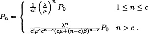
10.3.3   M/M/c/K Finite-Capacity Queueing System

In this queueing model, the system has a finite capacity of size K and we assume that c < K. The departure rates are state dependent and are given by:

Figure 10.11   M/M/c/K queueing system

The state transition diagram for this system is shown in Figure 10.11.

As evaluated before, the steady state probability of the system is given by:

Using the fact we get

where

Further, the average number of customers in the queue is given by:

Using Little’s formula, we can evaluate

where _eff = (1 − P_K).

10.3.4 M/M/∞ Queueing System

This is a Markovian queueing model without any queue. There are infinitely many servers such that every incoming customer finds an idle server immediately. The state transition diagram for this loss system is shown in Figure 10.12.

One can easily obtain the stationary distribution P_n as given by:

This follows a Poisson distribution with parameter ρ. Hence, the mean and variance of the number of customers in the steady state are the same as ρ.

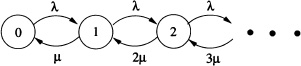
Figure 10.12   M/M/∞ system

Since there is no queueing in the M/M/∞ system, all waiting times are zero and the mean sojourn time in the system equals 1/μ. This means that all customers passing through such a system independently spend an exponentially distributed time.

One can observe that the expression of P₀ for the M/M/∞ queue is the limit of the respective expression for the M/M/c/c model as c tends to infinity. Further, the stationary distribution for the M/M/c/c queue converges to the stationary distribution of M/M/∞ for increasing c.

EXAMPLE 10.14

Consider a buffet served in a large area. The diners serve themselves. It is observed that a diner arrives every 10 seconds following a Poisson process and it takes about of a minute on average for the diner to serve himself. Find the average number of customers serving themselves and the average time spent.

Solution: According to the question, = 6 per minute and μ = 8 per minute. Hence The steady state probability of the system is:

Hence the average number of customers serving themselves is:

L_s = ρ = 0.75.

The average time spent in the system is:

T_s = 0.1250 minutes.   

10.4   NON-MARKOVIAN MODELS

In the previous sections, various characteristics for Markovian models were studied. In Markovian models, the analysis is conducted using the memoryless property of exponential distribution. In this section, we study non-Markovian models which exhibit a memoryless property only at certain time epochs. These random time epochs at which the system probabilistically restarts itself are known as regeneration time points. At regeneration time points, the memory of the elapsed time is erased. The times between the regeneration time points constitute an embedded renewal sequence. We deal with specific non-Markovian models such as M/G/1, GI/M/1, M/G/1/N and GI/M/1/N, where G represents a general or arbitrary distribution.

10.4.1   M/G/1 Queueing System

Definition 10.4 (M/G/1 Queueing System) This system is a type of M/M/1/∞ queue where service times follow a general distribution. Assume that the interarrival time follows an exponential distribution with mean and the distribution of service time is F(t) with pdf f(t) and mean .

Theorem 10.6 Consider X_t as the number of customers in the system at time t in the M/G/l queueing system. Let ρ = . Prove that, for ρ < 1, the generating function V(z) for the steady state probabilities are given by:

This is known as the Pollaczek-Khinchin (P-K) formula.

Proof :   Observe that the state of the system after an arrival of a customer depends not only on the number of the customers X_t at that time but also on the remaining service time of the customer receiving service, if any. Also note that the state of the system after a service completion depends only on the state of the system at that time.

Let X_n be the number of customers in the system at the departure instant of the nth customer. Let t_n denote the departure instant of the nth customer. Suppose Y_t = X_n, t_n ≤ t < t_n+1. Then, by Definition 9.49, {Y_t;t ≥ 0} will be a semi-Markov process having embedded discrete-time Markov chain (DTMC) {X_n,n = 0,1, · · ·}.

To obtain steady state probabilities of Y_t, we need to compute the transition probabilities of the embedded DTMC {X_n; n = 0,1, · · ·}. Since these points t_n are the regeneration points of the process {X_t;t ≥ 0}, the sequence of points {t_n; n = 0,1, · · ·} forms a renewal process.

Let A_n be a random variable denoting the number of customers who arrive during the service time of the nth customer. We have:

Since service times of all the customers, denoted by S, have the same distribution, the distribution of A_n is the same for all n. Denote, for all n,

Therefore:

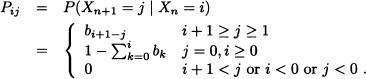
Denoting P = [P_ij], we have:

Note that {X_n, n = 0,1,· · ·} is an irreducible Markov chain. When ρ = < 1, the chain is positive recurrent. Hence the Markov chain is ergodic. The limiting probabilities

exist and are independent of the initial state i. The probability vector υ = [υ₀, υ₁, · · ·] is given as the unique solution of υ = υP and υ_j = 1. The solution can be obtained by using the generating functions of υ_j’s and a_j’s.

Define:

Here, f*(s) is the Laplace transform of f(t).

The expected number of arrivals is given by:

From υ = υP, we get:

Multiplying by z_j on both sides and taking the sum, we get:

Using V(1) = A(1) = 1,

provided A′(1) is finite and less than 1. Taking ρ = A′(1) < 1 we get υ₀ = 1−ρ. Hence:

Note 10.12 The average number of customers in the system in the steady state is given by:

This is known as the P-K mean value formula. Here, E(S²) is the second-order moment about the origin for the service time. This result holds true for all scheduling disciplines in which the server is busy if the queue is nonempty. When is the variance of the service time distribution, we get:

Note 10.13 In this derivation, we assume FIFO scheduling to simplify the analysis. However, the above formulas are valid for any scheduling discipline in which the server is busy if the queue is nonempty, no customer departs from the queue before completing service and the order of service is not dependent on the knowledge about service times. Hence, using Little’s formula, the average time spent in the system can be calculated.

Note 10.14 Using the P-K mean value formula, other measures such as L_q, T_q and T_s can be obtained as follows:

The formula states that mean waiting time is given by:

Hence, the average time spent in the system is

Note 10.15 (M/D/1 Queue) When the service time is a constant, i.e., the service time follows a deterministic distribution, = 0 and the P-K formula reduces to

where ρ = /μ and 1/μ is the constant service time.

Note 10.16 (M/M/1 Queue) When service time is exponentially distributed with mean and :

EXAMPLE 10.15

Consider Example 10.3. Assume that customers arrive in a Poisson process at an average rate of 100 per hour. Also assume that the time taken (in seconds) for each reservation by a computer server follows a uniform distribution with parameters 20 and 30.

(a) Find the average waiting time of the customers.

(b) Find the probability that the system is empty in the long run.

Solution: The arrival rate is = and the average service time is = 25 seconds. Hence ρ = .

(a) By using the P-K mean formula and Little’s formula, the average waiting time evaluates to 42.044.

(b) The probability that the system is empty in the long run is:

υ₀ = 1 − ρ = 0.30556.     

EXAMPLE 10.16

Consider an automatic transaction machine (ATM) with only one counter. Assume that the customers arrive according to a Poisson process with 5 customers per hour and may wait outside the counter if the ATM is busy. If the service time for the customers follows Weibull(2, ), determine L_s and T_q.

Solution: This problem is modeled as a M/G/1 queueing system with = 5 per hour and 1/μ = 0.0886. In this case, service time S follows Weibull(2, ). Using Theorem 4.5, we have E(S) = 0.0886 and Var(S) = 0.01785.

Using the P-K mean formula in equation (10.19), we get:

L_s = 1.02.

Then, using Little’s formula, we get:

10.4.2 GI/M/1 Queueing System

The model to be studied next is the GI/M/1 model in which the arrivals are independent and interarrival times follow a general distribution, but service times follow a Markovian property. Assume that the cdf of the interarrival time is F(t) with mean . Consider X_t as the number of customers in the system at time t. Note that the state of the system after the service completion of a customer depends not only on the state of the system X_t at that time but also on the remaining arrival time of the next customer, if any. However, the state of the system after the arrival of a customer depends only on the state of the system at that time.

Let X_n be the number of customers in the system at the arrival instant of the nth customer. Suppose t_n is the instant at which the nth customer arrives. Since these points t_n are the regeneration points of the process {X_t; t ≥ 0}, the sequence of points {t_n; n = 0, 1, 2, ···} forms a renewal process. Then {X_n; n = 0,1, · · ·} is an embedded Markov chain with state space S′ = {1, 2, · · ·}. By Definition 9.52, {X_t; t ≥ 0} is a Markov regenerative process having embedded Markov chain {X_n; n = 0,1, · · ·}.

Let A_n be the number of customers served during the interarrival time of the (n + l)th arrival. We then have:

X_n+1 = X_n + 1 − A_n     where     A_n ≤ X_n + 1, X_n ≥ 0.

Since the interarrival times are assumed to be independent and have the same distribution, the distribution of A_n is the same for all n. Denote for all n:

Therefore:

The transition probability matrix is given by:

When the embedded DTMC is irreducible and ergodic, the limiting probabilities that an arrival finds n in the system, denoted by π_n, n = 0, 1, 2, · · · are given as the unique solutions of

which gives:

Denoting zπ_i = π_i+1, we obtain for i ≤ 1:

π_i−1(z − b₀ − zb₁ − z²b₂ − ···) = 0.

Thus, for a nontrivial solution

it becomes

G(z) = z

where G(z) is the probability generating function of the {b_n}. It can be shown that G(z) = F*(μ(1 − z)), where F*(z) is the Laplace-Steiltjes transform of the interarrival time cdf F(t). Hence, the above equation may also be written as:

The condition ρ = < 1 is a necessary and sufficient condition for the existence of the stationary solution (refer to Gross and Harris, 1998). When ρ < 1, the stationary probability of n in the system just prior to an arrival is given by

where r₀ is the positive root between 0 and 1 of equation (10.20).

Note 10.17 It may be noted that this state distribution will be the equilibrium distribution that will be seen if the system is examined just before the instant of arrival of a customer to the system.

Note 10.18 Consider an arrival to the GI/M/1 queue. Let W be a random variable denoting the waiting time in the queue. It takes the value zero if an arriving customer finds the system to be empty on arrival (with probability π₀). If an arriving customer finds n jobs in the system (including the one currently in service), then the customer must wait for all of them to get served before his own service can begin. Note that the residual service time for the job that is currently in service also follows an exponential distribution. The mean waiting time in the queue, denoted by T_q, is given by:

Note that the mean results will be the same regardless of the service discipline being followed other than the FIFO discipline.

The waiting time distribution can be obtained using conditional distributions. Note that a customer who finds n customers in the system (including the one in service) on his/her arrival will encounter a random waiting time that will be equal to the sum of n independent exponentially distributed random variables. From this conditional distribution, the waiting time distribution is given by:

EXAMPLE 10.17

In a mobile handset manufacturing factory, a component arrives for testing every 3 seconds. It is assumed that the time (in seconds) for testing the component is exponentially distributed with parameter 4.

(a) Find the waiting time distribution of a component in the queue.

(b) Find the probability that there are no components available for testing in the long run.

Solution: Given = and μ = 4.

(a) Using equation (10.21), the probability distribution of the waiting time of a component in the queue is:

(b) The long-run probability that the system is empty is π₀ = (1 − b₀) where b₀ = e^−4t dt = 0.25.     

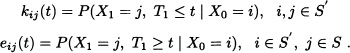
10.4.3 M/G/1/N Queueing System

The non-Markovian queueing model to be discussed next is a finite-capacity non-Markovian queueing model. The first model in this list is the M/G/1/N queueing model. This is similar to M/G/1, but now the system capacity is restricted to N.

The analysis of the M/G/1/N queue is similar to that of the M/G/1/∞ queue. But the main results of the M/G/1/∞ queue will not be applicable to the M/G/1/N queue. Let us examine the results for the M/G/1/N queue in detail. Let X_t denote the number of customers in the system at time t. Let T_n, n = 1, 2, ···, be the random variable denoting the departure time instants of the nth customer.

The P-K formula will no longer be applicable to the M/G/1/N queue as the expected number of arrivals during a service period will depend on the system size. Note that the number of customers in the M/G/1/N system constitutes a Markov regenerative process {X_t; t ≥ 0} with S = {0,1, · · ·, N} and embedded Markov chain where t_n is the nth customer departure instant and the corresponding number of customers left behind in the system by the departing customer. {X_n; n = 0,1, · · ·} is an embedded Markov chain (EMC) with state space S′ = {0, 1, 2, · · ·, N − 1}.

The one-step transition probability matrix is now truncated at N − 1 since we are observing the state just after a departure. Using P given in (10.18), it is given by

where the a’s are defined in (10.17). Assume that {X_n, n = 1, 2, · · ·} is irreducible, aperiodic and positive recurrent. Then the steady state probability vector υ = (υ_k) of the embedded Markov chain is given by

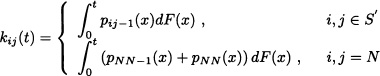
where P = K(∞) is the transition probability matrix of the EMC. Define the matrix (E_i,j(t))_{iS′, jS} as follows:

E_i,j(t) = P(X_t = j, T₁ > t | X₀ = i)

Finally, the steady state probabilities for M/G/1/N are

where

EXAMPLE 10.18

A machine is used for packing items. The machine can pack at most 2 items at a time. Items arrive as a Poisson process with rate = 2. The time required for packing an item follows a general distribution. Find the steady state probability of the system when the time required for packing follows a Weibull(2,1/2).

Solution: Let X_t be the number of items for packing at time t. The system can be modeled as a M/G/1/2 queueing system where each state represents a number of items for packing. Using the MRGP theory as defined in Section 9.4, we obtain the steady state probabilities. In this model, service completion time instants are the only regeneration time points. Hence, the time points of entering into states 0 and 1 are the only regeneration time instants. Therefore, in this case S′ = {0,1} and S = {0, 1, 2}. When service time follows a Weibull(2, ):

F(t) = 8te^−4t2, t ≥ 0.

Define the stochastic process {Y_t, t ≥ 0} during two successive regenerative time instants. Then {Y_t; t ≥ 0} is a CTMC which is known as the subordinated CTMC of the Markov regenerative process {X_t; t ≥ 0}. Let p_ij(t) be the probability that Y_t = j given that Y₀ = i. We first obtain the global and local kernel. The global kernel is defined as

K(t) = [k_ij(t)],i, j S′,

where

and the local kernel is given by , where:

e_ij(t) = P(X₁ = j, T₁ ≥ t | X₀ = i) = p_ij(t)(1 − F(t)), i S′, j S.

Here F(t) is the cumulative distribution function of the general distribution and p_ij(t) are the time-dependent probabilities of the subordinated CTMC and are evaluated as:

With this, the elements of K(t) are evaluated as:

Substituting = 2, we get:

Then the steady state probability vector υ = (υk) of the EMC is

where P = K(∞) is the transition probability matrix of the EMC. Solving, we get υ₀ = υ₁ = 1/2.

Now, the matrix E = [e_i,j(t), i S′, j S}:

Substituting = 2 and using α_i,j = e_i,j(t)dt, we get:

α₀₀ = 0.2728
α₀₁ = 0.1136
α₀₂ = 0.0567
α₁₀ = 0
α₁₁ = 0.2728
α₁₂ = 0.1703.

Finally, we compute the steady state probabilities for the M/G/1/N as given below:

where β₀ = β₁ = . Hence:

π₀ = 0.3078,   π₁ = 0.436,   π₂ = 0.2562.     

10.4.4 GI/M/1/N Queueing System

This queueing model is similar to GI/M/1, but now the system capacity is restricted to N. Let X_t denote the number of customers in the system at time t. Let T_n, n = 1, 2,···, be the random variable denoting the arrival time instant of the nth customer. Here, the arrival time instants are the only regeneration time epochs. Hence, {X_t; t ≥ 0} is not a semi-Markov process, but a MRGP with {X_n; n = 1, 2, · · ·} is an embedded Markov chain. S = {0, 1, 2,···, N} is the set of states at all time instants, and S′ = {1, 2, · · ·, N} is the set of states only at regeneration time instants. Following the theory of MRGP, we now proceed to determine the global kernel K(t) and local kernel E(t) matrices for the process. The elements of the global and local kernel are defined as:

The global kernel matrix is

where

and the p_ij’s are the transition probabilities of the subordinated CTMC. The state transition diagram for the subordinated CTMC is shown in Figure 10.13. The local kernel matrix is

Figure 10.13   Subordinated CTMC

where e_ij(t) = p_ij(1 − F(t)).

The limiting behavior is obtained by taking the limit as t approaches infinity. We require two new process characteristics to be defined, i.e., α_ij, the mean time spent by the MRGP in state j between two successive regeneration instants, given that it started in state i after the last regeneration,

and the steady state probability vector υ = [υ_k] of the EMC,

where P = K(∞) is the transition probability matrix of the embedded Markov chain. Then the steady state probability of the MRGP is given by

where β = .

Now, let us discuss the time-dependent behavior of the G/M/1/N queueing system. Define V(t) = (V_ij(t)) as the matrix of conditional state probabilities of the MRGP and the following equations for V(t) are matrix equations and

V_ij(t) = P{X_t = j | X₀ = Y₀ = i}, i,j S,

where {Y_n, n ≥ 0} is the embedded Markov chain of the MRGP {X_t; t ≥ 0}. Also,

where * denotes the convolution operator. The solution method for the time-dependent state distribution is outlined below:

1. Calculate K(t) and E(t).
2. Compute (s) and (s) where (s) and (s) are the Laplace-Steiltjes transform obtained as:
   

   

3. Solve the following linear system for (s):
   

   [I − (s)](s) = (s)

   where

   

4. Using inverse Laplace transforms, invert (s) to obtain V(t).
5. Using p(t)_1×S = p(0)_1×S′ V(t)_S′×S, obtain the time-dependent state probabilities of the MRGP.

EXAMPLE 10.19

Consider a system of two communicating satellites. The lifetime of a satellite follows an exponential distribution with parameter whereas the time to repair and resend the satellite follows a general distribution with mean 1/μ. Our interest is to determine the steady state probabilities when time to repair and resend the satellite follows a Weibull(2,1/2) distribution. Next we analyze a special case of the GI/M/1/N queue with N = 2. In this queueing model the arrival time instants are the only regeneration time instants. Hence, the time points of entering into the states 1 and 2 are the only regeneration time instants. Therefore, in this case S′ = {1, 2} and S = {0, 1, 2}. We solve this MRGP by taking F as Weibull(2, ). Here interarrival time is Weibull(2, ). Hence:

F(t) = 8te^−4t2, t ≥ 0.

Proceeding as above, we first evaluate the global and local kernel for this MRGP. The global kernel is defined as

K(t) = [k_ij(t)], i, j S′,

where

and the local kernel is given by

E(t) = [e_ij(t)] = [e_ij(t)]_{S′, jS,}

where

e_ij(t) = p_ij(t)(1 − F(t)).

Here F(t) is the cumulative distribution function of the Weibull distribution and p_ij(t) are the time-dependent probabilities of the subordinated CTMC and are evaluated as:

With this, the elements of K(t) are evaluated as:

Substituting μ = 2, we get:

Then the steady state probability vector υ = (υ_k) of the EMC is

where P = K(∞) is the transition probability matrix of the EMC. Solving, we get υ₀ = υ₁ = 1/2. Now, the matrix E = [e_i,j(t), i S′, j S]:

e₁₀(t)   =   (1 − e^−μt) e^−4t2
e₁₁(t)   =   e^−μt−4t2
e₁₂(t)   =   0
e₂₀(t)   =   (1 − e^−μt − μte^−μt) e^−4t2
e₂₁(t)   =   μte^−μt−4t2
e₂₂(t)   =   e^−μt−4t2.

Substituting μ = 2 and using α_i,j = e_i,j(t)dt, we get:

α₁₀ = 0.1703
α₁₁ = 0.2728
α₁₂ = 0
α₂₀ = 0.0567
α₂₁ = 0.1136
α₂₂ = 0.2728.

The steady state probabilities for the GI/M/1/2 are given as

where β₀ = β₁ = . Hence:

π₀ = 0.2561,   π₁ = 0.436,   π₂ = 0.3078.     

Queueing modeling is an important tool used to evaluate system performance in communication networks. It has a wide spectrum of applications in science and engineering. In this chapter we have studied some simple queueing models. For advanced queueing models such as non-Markovian, bulk and priority queues and queueing networks, the reader may refer to Gross and Harris (1998), Medhi (2003), Bhat (2008), and Bolch et al. (2006).

EXERCISES

10.1   Find the service rate for a M/M/1 queue where customers arrive at a rate of 3 per minute, given that 95% of the time the queue contains less than 10 customers.

10.2   The arrival of a patient at a doctor’s clinic follows a Poisson process with rate 8 per hour. The time taken by the doctor to examine a patient is exponential distribution with mean 6 minutes. Given that no patients are returned, find:

a) Probability that the patient has to wait on arrival.

b) Expected total time spent (including the service time) by any visiting patient.

10.3   It is assumed that the duration (in minutes) of a telephone conversation at a telephone booth consisting of only one telephone follows an exponential distribution with parameter μ = . If a person arrives at the telephone booth 3 minutes after a call started, then find his expected waiting time.

10.4   There are two servers at a service center providing service at an exponential rate of two services per hour. If the arrival rate of customers is 3 per hour and the system capacity is at most 3, then:

a) Find the fraction of potential customers that enter the system?

b) If there was only a single server with service rate twice as fast, i.e., μ = 4, then what will be the value of part (a)?

10.5   There are N spaces in a parking lot. Traffic arrives in a Poisson process with rate , but only as long as empty spaces are available. The occupancy times have an exponential distribution with mean 1/μ. If X_t denotes the number of occupied parking spaces at any time t, then:

a) Determine infinitesimal generator matrix Q and the forward Kolmogorov equations for the Markov process {X_t; t ≥ 0}.

b) Determine the limiting probability distribution of the stochastic process {X_t; t ≥ 0}.

10.6   An automobile emission inspection station has three inspection stalls, each with room for only one car. It is assumed that when a stall becomes vacant, the car standing first in the waiting line pulls up to it. Only four cars are allowed to wait at a time (seven in the station). Arrival occurs in a Poisson way with mean of one car per minute during the peak periods. The service time is exponential with mean 6 minutes.

1. Determine the average number of cars in the system during peak periods.
2. Determine the average waiting time (including service).

10.7   Show that the average time spent in a M/M/1 system with arrival rate and service rate 2μ is lesser than the average time spent in a M/M/2 system with arrival rate and each having service rate μ which is lesser than the average time spent in two independent M/M/1 queues with each having arrival rate /2 and equal service rate μ.

10.8   Suppose that you arrive at an ATM to find seven others, one being served (first-come-first-service basis) and the other six waiting in line. You join the end of the line. Assume that service times are independent and exponentially distributed with rate μ.

a) Model this situation as a birth-and-death process.

b) What is the expected amount of time you will spend in the ATM?

10.9   A telephone switching system consists of c trunks with an infinite caller population. Calls arrive in a Poisson process with rate and each call holding time is exponentially distributed with average l/μ. Let ρ = /μ. It is assumed that an incoming call is lost if all the trunks are busy.

a) Draw the state transition diagram for the system.

b) Derive an expression for π_n, the steady state probability that n trunks are busy.

c) Also find the number of trunks n, such that π_n ≤ 0.001.

10.10   For the M/M/1/N queueing system, show that as limit N → ∞ there are two possibilities: either ρ < 1 and P converges to the stationary distribution of the M/M/1 queue or ρ ≥ 1 and P goes to infinity.

10.11   Consider a telephone switching system with N subscribers. Each subscriber can attempt a call from time 0. Assume that there are c (< N) channels in the telephone switching system to handle the calls and assume that each call needs one channel. Assume that the arrival of a call from each customer follows a Poisson process with rate and each call duration follows an independent exponential distribution with rate μ.

a) Draw the state transition diagram for this queueing system.

b) Suppose that c = 10. Find such that no call is waiting.

10.12   For an M/M/c/∞ queue, prove that the distribution of waiting time in the queue is given by

and

fW_q (t) = cμ P_c e−^(cμ−)t, 0 < t < ∞.

10.13   A toll bridge with c booths at the entrance can be modeled as a c server queue with infinite capacity. Assuming the service times are independent exponential random variables with mean 1 second, sketch the state transition diagram for a continuous-time Markov chain for the system. Find the limiting state probabilities. What is the maximum arrival rate such that the limiting state probabilities exist?

10.14   Assume that taxis are waiting outside a station, in a queue, for passengers to come. Passengers for these taxis arrive according to a Poisson process with an average of 60 passengers per hour. A taxi departs as soon as two passengers have been collected or 3 minutes have expired since the first passenger has got in the taxi. Suppose you get in the taxi as the first passenger. What is your average waiting time for the departure?

10.15   Consider a Markovian queueing model with finite population, say N. In reliability theory, this model is known as the machine repair problem. In this case, customers are treated as N machines which are prone to failure. The lifetime of each machine is assumed to be exponentially distributed with parameter . There are c repairmen who repair the broken machines sequentially. The repair times are assumed to be exponential distributions with parameter μ. Obtain the steady state probabilities for this system.

10.16   For an M/M//N queueing system, show that the waiting time distribution W(t) is

where P_n, n = 0,1, · · ·, N − 1, is the steady state probability.

10.17   Find the stationary distribution for a M/M/c/c/K loss system with K population.

10.18   Consider a M/E_k/1 queueing system with arrival rate and mean service time . Let ρ = . Then show that the probability generating function of the distribution of the system state in equilibrium is given by: