CHAPTER 11

STOCHASTIC CALCULUS

Stochastic calculus plays an essential role in modern mathematical finance and risk management. The objective of this chapter is to develop conceptual ideas of stochastic calculus in order to provide a motivational framework. This chapter presents an informal introduction to martingales, Brownian motion, and stochastic calculus. Martingales were first defined by Paul Lévy (1886–1971). The mathematical theory of martingales has been developed by American mathematician Joseph Doob (1910–2004). We begin with the basic notions of martingales and its properties.

11.1   MARTINGALES

The martingale is a strategy in a roulette game in which, if a player loses a round of play, then he doubles his bet in the following games so that if he wins he would recover from his previous losses. Since it is true that a large losing sequence is a rare event, if the player continues to play, it is possible for the player to win, and thus this is apparently a good strategy. However, the player could run out of funds as the game progresses, and therefore the player cannot recover the losses he has previously accumulated. One must also take into account the fact that casinos impose betting limits.

Formally, suppose that a player starts a game in which he wins or loses with the same probability of . The player starts betting a single monetary unit. The strategy is progressive where the player doubles his bet after each loss in order to recoup the loses. A possible outcome for the game would be the following:

Bet                   1    2    4    8    16     1    1

Outcome          F    F    F    F    W    W   F

Profit              -1   -3   -7   -15   1     2    1

Here W denotes “Win” and F denotes “Failure”. This shows that every time the player wins, he recovers all the previous losses and it is also possible to increase his wealth to one monetary unit. Moreover, if he loses the first n bets and wins the (n + l)th, then his wealth after the nth bet is equal to:

This would indicate a win for the player. Nevertheless, as we shall see later, to carry out this betting strategy successfully, the player would need on average infinite wealth and he would have to bet infinitely often (Rincón, 2011).

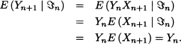
In probability theory, the notion of a martingale describes a fair game. Suppose that the random variable X_m denotes the wealth of a player in the mth round of the game and the σ-field _m has all the knowledge of the game at the mth round. The expectation of X_n (with n ≥ m), given the information in _m, is equal to the fortune of the player up to time m. Then the game is fair. Using probability terms, we have, with probability 1:

E(X_n | _m) = X_m for all m ≤ n.

A stochastic process {X_t;t ≥ 0} satisfying the above equation is called a discrete-time martingale. Formally we have the following definitions:

Definition 11.1 Let (Ω, , P) be a probability space. A filtration is a collection of sub-σ-algebras (_n)_n≥0 of such that _m ⊆ _n for all m ≤ n. We say that the sequence {X_n;n ≥ 0} is adapted to the filtration (_n)_n≥0 if for each n the random variable X_n is _n-measurable, that is, {ω Ω : X_n(ω) ≤ a} _n for all a .

Definition 11.2 Let {X_n;n ≥ 0} be a sequence of random variables defined on the probability space (Ω, , P) and (_n)_n≥0 be a filtration in . Suppose that {X_n;n ≥ 0} is adapted to the filtration (_n)_n≥0 and E(X_n) exists for all n. We say that:

(a) {X_n;n ≥ 0} is a (_n)_n-martingale if and only if E(X_n | _m) = X_m a.s. for all m ≤ n.

(b) {X_n;n ≥ 0} is a (_n)_n-submartingale if and only if E(X_n | _m) ≥ X_m a.s. for all m ≤ n.

(c) {X_n;n ≥ 0} is a (_n)_n-supermartingale if and only if E(X_n | _m) ≤ X_m a.s. for all m ≤ n.

Note 11.1 The sequence {X_n;n ≥ 0} is obviously adapted to the canonical filtration or natural filtration. That is to say that the filtration (_n)_n≥0 is given by _n = σ (X₁, X₂, · · ·, X_n), where σ (X₁, X₂, · · ·, X_n) is the smallest σ-algebra with respect to which the random variables X₁,X₂,· · ·,X_n are _n-σ-measurable. When we speak of martingales, supermartingales and submartingales, with respect to the canonical filtration, we will not explicitly mention it. In other words, if we say: “(X_n)_n is a (sub-, super-) martingale” and we do not reference the filtration, it is assumed that the filtration is the canonical filtration.

Note 11.2 If {X_n;n ≥ 0} is a (_n)_n-martingale, it is enough to see that:

E(X_n+1) | _n) = X_n for all n .

Note 11.3 If {X_n;n ≥ 0} is a (_n)_n-submartingale, then {−X_n;n ≥ 0} is a (_n)_n-supermartingale. Thus, in general, with very few modifications, every proof made for submartingales is also valid for supermartingales and vice versa.

EXAMPLE 11.1

Let {X_n;n ≥ 0} be a martingale with respect to (_n)_n≥0 and (_n)_n≥0 be a filtration such that _n ⊆ _n for all n. If X_n is _n-measurable, then {X_n;n ≥ 0} is a martingale with respect to (_n)_n. Indeed:

Therefore, every (_n)_n-martingale is a martingale with respect to the canonical filtration.          

EXAMPLE 11.2 Random Walk Martingale

Let Z₁, Z₂, · · · be a sequence of i.i.d. random variables on a probability space (Ω, , P) with finite mean μ = E (Z₁), and let _n = σ(Z₁, · · ·, Z_n), n ≥ 1. Let X_n = Z₁ + · · · + Z_n, n ≥ 1. Then, for all n ≤ 1,

so that:

Thus, {X_n;n ≤ 1} is a martingale if μ = 0, a submartingale if μ > 0 and a supermart ingale if μ < 0.          

EXAMPLE 11.3 Second-Moment Martingale

Let Z₁, Z₂, · · · be a sequence of i.i.d. random variables on a probability space (Ω, , P) with finite mean μ = E (Z₁) and variance σ² = Var(Z₁). Let _n = σ(Z₁,· · ·, Z_n), n ≥ 1. Let and . It is easily verified that {Y_n;n ≥ 1} is a submartingale and is a martingale. Assume:

EXAMPLE 11.4

Let X₁,X₂,· · · be a sequence of independent random variables with E (X_n) = 1 for all n. Let {Y_n;n ≥ 1} be:

If _n = σ(X₁,· · ·, X_n), it is clear that:

That is, {Y_n;n ≥ 1} is a martingale with respect to (_n)_n.          

EXAMPLE 11.5 Polya Urn Model

Suppose that an urn has one red ball and one black ball. A ball is drawn at random from the urn and is returned along with a ball of the same color. The procedure is repeated many times. Let X_n denote the number of black balls in the urn after n drawings. Then X₀ = 1 and {X_n;n ≥ 0} is a Markov chain with transitions

and

Let be the proportion of black balls after n drawings. Then {M_n;n ≥ 0} is a martingale, since:

EXAMPLE 11.6 Doob’s Martingale

Let X be a random variable with E(|X|) < ∞, and let {_n}_n≥1 be a filtration. Define X_n = E(X | _n) for n ≥ 1. Then {X_n,n ≥ 0} is a martingale with respect to {_n}_n≥0:

Also,

As we know that every martingale is also a submartingale and a supermartingale, the following theorem provides a method for getting a submartingale from a martingale.

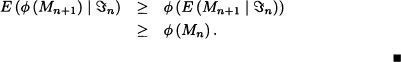
Theorem 11.1 Let {M_n;n ≥ 0} be a martingale with respect to the filtration (_n)_n≥0. If (·) is a convex function with E(|(M_n)|) < ∞ for all n, then {(M_n);n ≥ 0} is a submartingale.

Proof: By Jensen’s inequality (Jacod and Protter, 2004):

EXAMPLE 11.7

Let {M_n;n ≥ 0} be a nonnegative martingale with respect to the filtration (_n)_n≥0. Then and {−log M_n;n ≥ 0} are submartingales.          

EXAMPLE 11.8

Let {Y_n;n ≥ 1} be an arbitrary collection of random variables with E[|Y_n|] < ∞ for all n ≥ l. Let _n = σ (Y₁, · · ·, Y_n), n ≥ 1. For n ≥ 1, define

where ₀ = {,Ω}. Then, for each n ≥ 1, X_n is _n-measurable with E[|X_n|] < ∞. Also, for n ≥ 1:

Hence {X_n;n ≥ 1} is a martingale. Thus, it is possible to construct a martingale sequence starting from any arbitrary sequence of random variables.          

EXAMPLE 11.9

Let {X_n;n ≥ 0} be a martingale with respect to the filtration (_n)_n≥0 and let {Y_n;n ≥ 0} be defined by:

Y_n+1 := X_n+1 − X_n, n = 0,1,2, · · ·.

It is clear that:

Suppose that {C_n;n ≥ 1} is a predictable stochastic process, that is, C_n is a _n−1-measurable random variable for all n. We define a new process {Z_n;n ≥ 0} as:

The process {Z_n;n ≥ 0} is a martingale with respect to filtration {_n}_n≥0 and is called a martingale transformation of the process Y, denoted by Z = C · Y. The martingale transforms are the discrete analogues of stochastic integrals. They play an important role in mathematical finance in discrete time (see Section 12.3).          

Note 11.4 Suppose that {C_n;n ≥ 1} represents the amount of money a player bets at time n and Y_n := X_n − X_n−1 is the amount of money he can win or lose in each round of the game. If the bet is a monetary unit and X₀ is the initial wealth of the player, then X_n is the player’s fortune at time n and Z_n represents the player’s fortune by using the game strategy {C_n;n ≥ 1}. The previous example shows that if {X_n;n ≥ 0} is a martingale and the game is fair, it will remain so no matter what strategy the player follows.

EXAMPLE 11.10

Let ξ₁, ξ₂ · · · be i.i.d. random variables and suppose that for a fixed t:

m(t) := E(e^tξ1) < ∞.

The sequence of random variables {X_n;n ≥ 0} with X₀ := 1 and

is a martingale.          

EXAMPLE 11.11

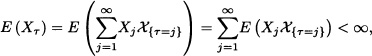
Let ξ₁,ξ₂ · · · and X_n (t) be as in the example above. We define the random variables as:

We have that is a martingale.          

Definition 11.3 A random variable with values {1,2, · · · }∪{∞} is a stopping time with respect to the filtration (_n)_n≥1 if { ≤ n} _n for each n ≥ 1.

Note 11.5 The condition given in the previous definition is equivalent to { = n} _n for each n ≥ 1.

EXAMPLE 11.12 First Arrival Time

Let X₁,X₂, · · · be a sequence of random variables adapted to the filtration (_n)_n≥1. Suppose that A is a Borel set of and consider the random variable defined by

τ := min {n ≥ 1 : X_n A}

with min () := ∞. It is clear that τ is a stopping time since:

In particular we have that, for the gambler’s ruin case, the time τ at which the player reaches the set A = {0, a} for the first time is a stopping time.          

EXAMPLE 11.13 Martingale Strategy

Previously we observed that if a player who follows the martingale strategy loses the first n bets and wins the (n + l)th bet, then his wealth X_n+1 after the (n + l)th bet is:

Suppose that τ is the stopping time at which the player wins for the first time. It is of our interest to know what is, on average, his deficit for that time. That is, we want to determine the value E(X_τ−1) from the previous equation. We have:

Therefore, on average, a player must have an infinite capital to fulfill the strategy.          

Let {X_n;n ≥ 1} be a martingale with respect to the filtration (_n)_n≥1. We know that E(X_n) = E(X₁) for any n ≥ 1. Nevertheless, if τ is a stopping time, it is not necessarily satisfied that τ. Our next objective is to determine the conditions under which τ, where τ is the stopping time.

Definition 11.4 Let τ be a stopping time with respect to the filtration (_n)_n≥0 and let {X_n;n ≥ 0} be a martingale with respect to the same filtration. We define the stopped process {X_τΛn;n ≥ 0} as follows:

Theorem 11.2 If {X_n;n ≥ 1} is a martingale with respect to (_n)_n≥0, and if τ is a stopping time with respect to (_n)_n≥0, then {X_τΛn;n ≥ 0} is a martingale.

Proof: Refer to Jacod and Protter (2004).          

Theorem 11.3 (Optional Stopping Theorem) Let {X_n;n ≥ 0} be a martingale with respect to the filtration (_n)_n≥1 and let τ be a stopping time with respect to (_n)_n≥1. If

1. τ < ∞ a.s.,

2. E(X_τ) and < ∞

3. ,

then E{X_τ) = E (X_n) for all n ≥ 1.

Proof: Since for any n ≥ 1 it is satisfied that

and since the process {X_n;n ≥ 0} and {X_τΛn;n ≥ 0} are both martingales, we have:

On the other hand by the hypothesis

and

it follows that the tail of the series, which is , tends to zero as n tends to ∞. Therefore, taking the limit as n → ∞ in (11.2), we obtain:

E(X_τ) = E(X_n) for all n ≥ 1.              

Note 11.6 Suppose that {X_n;n ≥ 0} is a symmetric random walk in with X₀ := 0 and that N is a fixed positive integer and let τ be the stopping time defined by:

τ := min {n ≥ 1 : |X_n| = N}.

It is easy to verify that the process {X_n;n ≥ 0} and the process are martingales. Moreover, it is possible to show that the stopping theorem hypotheses are satisfied. Consequently, we get

from which we have:

That is, the random walk needs on average N² steps to reach the level N.

The following results on convergence of martingales, which we state without proof, provide many applications in stochastic calculus and mathematical finance.

Theorem 11.4 Let{X_n;n ≤ 0} be a submartingale with respect to (_n)_n≥0 such that sup_n E(|X_n|) < ∞. Then there exists a random variable X having E(|X|) < ∞ such that:

Note 11.7 There is a similar result for supermartingales because if {X_n;n ≥ 0} is a supermartingale with respect to (_n)_n≥0, then {−X_n;n ≥ 0} is a submartingale with respect to (_n)_n≥0. The previous theorem implies in addition that every nonnegative martingale converges almost surely. The following example shows that, in general, there is no convergence in the mean.

EXAMPLE 4.14

Suppose that {Y_n;n ≥ 1} is a sequence if i.i.d random variables with normal distribution eac having mean 0 and variance σ². Let:

It is easy to prove that {X_n;n ≥ 0} is a nonnegative martingale. By using the strong law of large numbers we obtain that . Nevertheless, since E (X_n) = 1 for all n.          

Now we present a theorem which gives a sufficient condition to ensure the almost sure convergence and convergence in the r-mean. Its proof is beyond the scope of this text, (refer to Williams, 2006).

Theorem 11.5 If {X_n;n ≥ 0} is a martingale with respect to such that E(|X_n|^r) < ∞ for some r > 1, then there is a random variable X such that

X_n X

converges almost surely and in the r-mean.

Next, we give a brief account of continuous-time martingales. Many of the properties of martingales in discrete time are also satisfied in the case of martingales in continuous time.

Definition 11.5 Let (Ω, , P) be a probability space. A filtration is a family of sub-σ-algebras (_t)_tT such that _s ⊆ _t for all s ≤ t.

Definition 11.6 A stochastic process {X_t;t T} is said to be adapted to the filtration (_t)_tT if X_t is _t-_{measurable for each t} T.

Definition 11.7 Let ≠ T ⊆ . A process {X_t;t T} is called a martingale with respect to the filtration (_t)_tT if:

1. {X_t;t T} is adapted to the filtration (_t)_tT.

2. E(|X_t|) < ∞ for all t T.

3. E(X_t | _s) = X_s a.s. for all s ≥ t.

Note 11.8

a. If condition 3 is replaced by: E(X_t | _s) ≥ X_s a.s. for all s ≤ t, then the process is called a submartingale.

b. If condition 3 is replaced by: E (X_t | _s) ≤ X_s a.s. for all s ≤ t, then the process is called a supermartingale.

Note 11.9 Condition 3 in the previous definition is equivalent to:

E (X_t − X_s | _s) = 0 a.s. for all s ≤ t.

Note 11.10 The sequence {X_t;t ∈ T} is clearly adapted to the canonical filtration, that is, to the filtration (_t)_t∈T, where _t = σ (X_s, s ≤ t) is the smallest σ-algebra with respect to which the random variables X_s with s ≤ t are measurable.

EXAMPLE 11.15

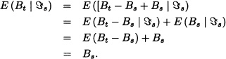
Let {X_t; t ≥ 0} be a process with stationary and independent increments. Assume _t = σ (X_s, s ≤ t) and E (X_t) = 0 for all t ≥ 0. Then:

That is, {X_t;t ≥ 0} is a martingale with respect to (_t)_t≥0.    

Note 11.11 If in the above example we replace the condition “E (X_t) = 0 for all t ≥ 0” by “E(X_t) ≥ 0 for all t ≥ 0” [“E (X_t) ≤ 0 for all t ≥ 0”] we find that the process is a submartingale (a supermartingale).

EXAMPLE 11.16

Let {N_t; t ≥ 0} be a Poisson process with parameter λ > 0. The process {N_t;t ≥ 0} has independent and stationary increments and in addition E(N_t) = λt ≥ 0. Hence, {N_t; t ≥ 0} is a submartingale.

However, the process {N_t − λt;t ≥ 0} is a martingale and is called a compensated Poisson process.    

11.2 BROWNIAN MOTION

The Brownian motion is named after the English botanist Robert Brown (1773–1858) who observed that pollen grains suspended in a liquid moved irregularly. Brown, as his contemporaries, assumed that the movement was due to the life of these grains. However, this idea was soon discarded as the observations remained unchanged by observing the same movement with inert particles. Later it was found that the movement was caused by continuous particle collisions with molecules of the liquid in which it was embedded. The first attempt to mathematically describe the Brownian motion was made by the Danish mathematician and astronomer Thorvald N. Thiele (1838–1910) in 1880. Then in the early twentieth century, Louis Bachelier (1900), Albert Einstein (1905) and Norbert Wiener (1923) initiated independently the development of the mathematical theory of Brownian motion. Louis Bachelier (1870–1946) used this movement to describe the behavior of stock prices in the Paris stock exchange. Albert Einstein (1879–1955) in 1905 published his paper “Über die von dev molekularischen Theorie der Wärme gefordete Bewegung von in ruhenden Flüssigkeiten suspendierten Teilchen” in which he showed that at time t, the erratic movement a particle can be modeled by a normal distribution. The American mathematician Norbert Wiener (1894–1964) was the first to perform a rigorous construction of Einstein’s model of Brownian motion, which led to the definition of the so-called Wiener measure in the space of trajectories. In this section we introduce Brownian motion and present a few of its important properties.

Definition 11.8 The stochastic process B = {B_t,t ≥ 0} is called a standard Brownian motion or simply a Brownian motion if it satisfies the following conditions:

1. B₀ = 0.
2. B has independent and stationary increments.
3. For s < t, every increment {B_t − B_s} is normally distributed with mean 0 and variance (t − s).
4. Sample paths are continuous with probability 1.

Note 11.12

1. The Brownian motion is a Gaussian process. This is because the distribution of a random vector of the form(B_t1, B_t2, … , B_tn) is a linear combination of the vector (B_t1, B_t2 − B_t1, …, B_tn − B_tn−1) which has normal distribution.
2. The Brownian motion is a Markov process with transition probability density function

   

   for any x, y ∈ and 0 < s < t.

   

   Figure 11.1 Sample path of Brownian motion

3. The probability density function of B_t is given by:

   

In the following algorithm, we simulate the sample path for the Brownian motion. This involves repeatedly generating independent standard normal random variables.

Algorithm 11.1

Input: T, N where T is the length of time interval and N is the time steps.

Output: BM(k) for k = 0(1)N.

Initialization: BM(0) := 0

Iteration: For k = 0(1)N − 1 do:
               Z(k + 1) = stdnormal(rand(0, 1))
               BM(k +1) = BM(K) + × Z(k + 1)

where stdnormal(rand(0, 1)) is the value of the standard normal random variable using the random number generated in the interval (0, 1). Using this algorithm, we obtain the sample path of Brownian motion as shown in Figure 11.1 for T = 10 and N = 1000.

Now we will discuss some simple and immediate properties of the Brownian motion:

1. E (B_t) = 0 for all t ≥ 0.
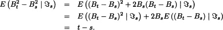
2. E = t for all t ≥ 0.
3. The covariance of Brownian motion C (s, t) = min (s, t). This is because, if s ≤ t, then:

   

   Similarly, if t ≤ s, we get C(s, t) = t. Hence, the covariance of Brownian motion C(s, t) = min (s, t).

Theorem 11.6 Let {B_t;t ≥ 0} be a Brownian motion. Then the following processes are also Brownian motions:

1. Shift Property: For any s > 0, = B_t+s − B_s is a Brownian motion.
2. Symmetry Property: = −B_t is a Brownian motion.
3. Scaling Property: For any constant c > 0, is a Brownian motion.
4. Time Reversal Property: for t > 0 with B₀ = 0 is a Brownian motion.

Proof: It is easy to check that {;t ≥ 0} for i = 1, 2, 3, 4 are processes with independent increments with = 0. Also the increments are normally distributed with mean 0 and variance (t − s).          

Brownian Motion as a Limit of Random Walks Let {X_t,t ≥ 0} be the stochastic process representing the position of a particle at time t. We assume that the particle performs a random walk such that in a small interval of time of duration Δt the particle moves forward a small distance Δx with probability p or moves backward by a small distance Δx with probability q = 1 − p, where p is independent of x and t. Suppose that the random variable Y_k denotes the length of the kth step taken by the particle in a small interval of time Δt and the Y_k’s are independent and identically distributed random variables with P(Y_k = +Δx) = p = 1 − P(Y_k = −Δx).

Suppose that the interval of length t is divided into n equal subintervals of length Δt. Then n · (Δt) = t, and the total displacement X_t of the particle is the sum of n i.i.d. random variables Y_k, so that

with n = [n(t)] and n(t) = t/Δt for each t ≥ 0. As a function of t, for each ω, X_t is a step function where steps occur every Δt units of time and steps are of magnitude Δx. We have:

E(Y_i) = (p − q)Δx  and  Var(Y_i) = 4pq(Δx)².

Then:

E(X_t) = n(p − q)Δx  and  Var(X_t) = 4npq(Δx)².

Substituting we have:

When we allow Δx → 0 and Δt → 0, the corresponding steps n tend to ∞.We assume that the following expressions have finite limits:

and

where μ and σ are constants. Since the Y_k’s are i.i.d. random variables, using the central limit theorem, for large n = n(t) the sum is asymptotically normal with mean μt and variance σ²t. That is,

where Z is a standard normal random variable.

Various Gaussian and non-Gaussian stochastic processes of practical relevance can be derived from Brownian motion. We introduce some of those processes which will find interesting applications in finance.

EXAMPLE 11.17

Let {B_t;t ≥ 0} be a Brownian motion. The stochastic process {R_t;t ≥ 0} defined by

is called a Brownian motion reflected at the origin. The mean and variance of R_t are given by:

EXAMPLE 11.18

Let {B_t;t ≥ 0} be a Brownian motion. The stochastic process {A_t;t ≥ 0} is defined by

where T₀ = inf{t ≥ 0 : B_t = 0} is the hitting time at 0. Then A_t is called the absorbed Brownian motion.    

EXAMPLE 11.19

The stochastic process {U_t; 0 ≤ t ≤ 1}, defined as

U_t = B_t − tB₁,

is called a Brownian bridge or the tied-down Brownian motion.

The name Brownian bridge comes from the fact that it is tied down at both ends t = 0 and t = 1 since U₀ = U₁ = 0. In fact, the Brownian bridge {U_t;0 ≤ t ≤ 1} is characterized as being a Gaussian process with continuous sample paths and the covariance function

Cov (U_s, U_t) = s(1 − t),     0 ≤ s ≤ t ≤ 1.

If{U_t;0 ≤ t ≤ 1} is a Brownian bridge, then it can be shown that the stochastic process

is the standard Brownian motion.    

EXAMPLE 11.20

Let {B_t;t ≥ 0} be a Brownian motion. For μ ∈ and σ > 0, the process

is called a Brownian motion with drift μ. It is easy to check that is a Gaussian process with mean fit and covariance C(s, t) = σ² min(s, t).    

EXAMPLE 11.21

Let {B_t;t ≥ 0} be a Brownian motion. For μ ∈ and σ > 0, the process

X_t = exp(μt + σB_t),     t ≥ 0,

is called a geometric Brownian motion.    

This process has been used to describe stock price fluctuations (see next chapter for more details). It should be noted that X_t is not a Gaussian process. Now we will give the mean and covariance for the geometric Brownian motion.

Using the moment generating function of the normal random variable (4.2), we get:

Similarly we obtain the covariance of the geometric Brownian motion for s < t,

and the variance is given by:

The previous section discussed continuous-time martingales. Presently we will see a Brownian motion as an example of a continuous-time martingale.

Theorem 11.7 Suppose that {B_t;t ≥ 0} is a Brownian motion with respect to filtration t, where _t := σ(B_s; s ≤ t). Then

1. {B_t} is a martingale,
2. { − t} is a martingale and
3. for , {exp(σB_t − (σ²/2)t)} is a martingale (called an exponential martingale).

Proof:

1. It is clear that, for every t ≥ 0, B_t is adapted to the filtration and E(B_t) exists. For any s, t ≥ 0 such that s < t:

   

2. 
   

   

   Thus:

   

3. The moment generating function of {B_t; t ≥ 0} is given by:

   

   Therefore and is integrable. Now:

   

Note 11.13 Let {X_t; t ≥ 0} be a stochastic process with respect to filtration . Then {X_t; t ≥ 0} is a Brownian motion if and only if it satisfies the following conditions:

1. X₀ = 0 a.s.
2. {X_t; t ≥ 0} is a martingale with respect to filtration .
3. is a martingale with respect to filtration .
4. With probability 1, the sample paths are continuous.

The above result is known as Lévy’s characterization of a Brownian motion (see Mikosh, 1998).

The possible realization of a sample path’s structure and its properties play a crucial role and are the subject matter of deep study. Brownian motion has the continuity of the sample path by definition. Another important property is that it is nowhere differentiable with probability 1. The mathematical proof of this property is beyond the scope of this text. For rigorous mathematical proof, the reader may refer to Karatzas and Shreve (1991) or Breiman (1992).

Now we will see an important and interesting property of a Brownian motion called quadratic variation. In the following, we define the notion of quadratic variation for a real-valued function.

Definition 11.9 Let f (t) be a function defined on the interval [0, T]. The quadratic bounded variation of the function f is

where is a partition of the interval [0,T],

with:

Theorem 11.8 The quadratic variation of the sample path of a Brownian motion over the interval [0, T] converges in mean square to T.

Proof: Let be a partition of the interval [0, T] :

Let

Then for each n we have:

Also:

We conclude that:

Thus we have proved that Q_n converges to T in mean square.     

We can also prove Q_n converges to T with probability 1. This proof can be found in Breiman (1992) and Karatzas and Shreve (1991) (see Chapter 8 for different types of convergence of random variables).

As we have seen in this section, the sample path of Brownian motion is nowhere differentiable. Because the stochastic processes which are driven by Brownian motion are also not differentiable, we cannot apply classical calculus. In the following section we introduce the stochastic integral or Itô integral with respect to Brownian motion and its basic rules. We will do so using an intuitive approach which is based on classical calculus. For a mathematically rigorous approach on this integral see Karatzas and Shreve (1991) or Oksendal (2006).

11.3 ITÔ CALCULUS

The stochastic calculus or Itô calculus was developed during the year 1940 by Japanese mathematician K. Itô and is similar to the classical calculus of Newton which involves differentials and integrals of deterministic functions. In this section, we will study the stochastic integral of the process {X_t; t ≥ 0} with respect to a Brownian motion, that is, we adequately define the following expression:

In the classical calculus, the equations which consist of the expressions of the form dx are known as differential equations. If we replace the term dx by an expression of the form dX_t, the equations are known as stochastic differential equations. Formally, a stochastic differential equation has the form

where μ(x, t) and σ(x, t) are given functions. Equation (11.10) can be written in integral form:

The first integral is a Riemann integral. How can we interpret the second integral? Initially we could take our inspiration from ordinary calculus in defining this integral as a limit of partial sums, such as

provided the sum exists. Unlike the Riemann sums, the value of the sum here depends on the choice of the chosen points t_i’s. In the case of stochastic integrals, the key idea is to consider the Riemann sums where the integrand is evaluated at the left endpoints of the subintervals. That is:

Observing that the sum of random variables will be another random variable, the problem is to show that the limit of the above sum exists in some suitable sense. The mean square convergence (see Chapter 8 for the definition) is used to define the stochastic integral. We establish the family of stochastic processes for which the Itô integral can be defined.

Definition 11.10 Let L² be the set of all the stochastic processes {X_t; t ≥ 0} such that:

(a.) The process X = {X_t; t ≥ 0} is progressively measurable with respect to the given filtration . This means that, for every t, the mapping (s, ω) → X_s(ω) on every set [0, t] × Ω is measurable.

(b.) for all T > 0.

Now we give the definition of the Itô integral for any process {X_t; t ≥ 0} ∈ L².

Definition 11.11 Let {X_t; t ≥ 0} be a stochastic process in L² and T > 0 fixed. We define the stochastic integral or Itô integral of X_t with respect to Brownian motion B_t over the interval [0, T] as

where is a partition of the interval [0, T] such that

with:

Notation:

EXAMPLE 11.22

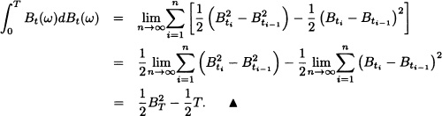
Consider the stochastic integral

where B_t is a Brownian motion. Let 0 = t₀ < t₁ < t₂ < … < t_n = T be a partition of the interval [0, T]. From the definition of the stochastic integral, we have:

By the use of the identity

We get:

The stochastic integral (11.12) for all T > 0 satisfies the following properties:

1. Zero mean:
   

   

2. Itô isometry:
   

   

3. Martingale: For t ≤ T,

   

4. Linearity: For {X_t; t ≥ 0}, {Y_t; t ≥ 0} ∈ L²,

Proof: We now prove only the martingale property of the Itô integral. For proofs of the remaining properties, the reader may refer to Karatzas and Shreve (1991). Consider

where the above equality follows by the zero mean property.     

EXAMPLE 11.23

Let be an Itô integral. We have E (X_t) = 0 by property (11.22). The variance is calculated by use of the mgf of Brownian motion and Itô isometry. We have:

In the context of ordinary calculus, the Itô formula is also known as the change of variable or chain rule for the stochastic calculus.

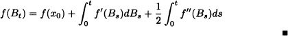
Theorem 11.9 (Itô’s Formula) Let be a twice-differentiable function and let B = {B_t; t ≥ 0} be a Brownian motion that starts at x₀, that is, B₀ = x₀. Then

or in the differential form:

Proof: Fix t > 0. Let be a partition of [0, t]. By Taylor’s theorem, we have:

Taking the limit n → ∞ when Δt → 0, we find that the first sum of the right- hand side converges to the Itô integral and the second sum on the right-hand side converges to because of mean square convergence. We get:

Thus:

EXAMPLE 11.24

Let f (x) = x² and B = {B_t; t ≥ 0} be a standard Brownian motion. The Itô formula establishes that:

That is:

EXAMPLE 11.25

Let f (x) = x³ and B = {B_t; t ≥ 0} be a standard Brownian motion. The Itô formula establishes that:

That is:

EXAMPLE 11.26

Let for a Brownian motion {B_t; t ≥ 0} with B₀ = 0. Prove that

and hence find and .

Solution. By the Itô’s formula, we have:

Taking expectation we have:

Since β₂(t) = t, we get:

Definition 11.12 For a fixed T > 0, the stochastic process {X_t;0≤ t ≤ T} is called an Itô process if it has the form

where X₀ is -measurable and the processes Y_t and Z_t are -adapted such that, for all t ≥ 0, E(|Y_t|) < ∞ and E(|Z_t|²) < ∞. An Itô process has the differential form

We now give the Itô formula for an Itô process.

Theorem 11.10 (Itô’s Formula for the General Case) Let {X_t; t ≥ 0} be an Itô process given in (11.14). Suppose that f (t, x) is a twice continuously differentiable function with respect to x and t. Then f(t, X_t) is also an Itô process and:

Proof: See Oksendal (2006).     

Note 11.14 We introduce the notation

which is computed using the following multiplication rules:

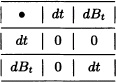
The Itô formula then can be expressed in the following form:

Note 11.15 Itô’s formula can also be expressed in differentials as:

EXAMPLE 11.27

Let X_t = t and f(t, x) = g (x) be a twice-differentiable function. It is easy to see that:

Thus, applying Itô’s formula, we get:

That is, the fundamental theorem of calculus is a particular case of Itô’s formula.     

EXAMPLE 11.28

Let X_t = h (t) where h is a differentiable function and let f (t, x) = g (x) be a twice-differentiable function. It is easy to check that:

Applying Itô’s formula, we obtain :

In this case also, the substitution theorem of calculus is a particular case of Itô’s formula.     

EXAMPLE 11.29

Let {B_t; t ≥ 0} be a Brownian motion and consider the following differential equation:

Let Z_t = log(y_t). Then, by Itô’s formula, we have:

Thus:

Integrating we get

so that the solution of equation (11.15) is:

EXAMPLE 11.30

Consider the Langevin equation

dX_t = −βX_tdt + αdB_t

where and β > 0. The process {X_t; t ≥ 0} with X₀ = x₀ can be written as:

Let f (t, x) = e^βtx. Applying Itô’s formula, we get:

Integration of the above equation gives for s ≤ t:

The solution of the Langevin equation with initial condition X₀ = x_o is called an Ornstein-Uhlenbeck process.     

We complete this chapter with the Itô formula for functions of two or more variables.

Multidimensional Itô Formula

We now give the Itô formula for functions of two variables. Consider a two-dimensional process

where and are two Brownian motions with their covariances given by

where ρ is the correlation coefficient of the two Brownian motions. Let g(t, x, y) be a twice-differentiable function and let Z_t = g(t, X_t, Y_t). Then Z_t is also an Itô process and satisfies:

For the proof, the reader may refer to Karatzas and Shreve (1991).

Note 11.16 For any two Itô processes, {X_t; t ≥ 0} and {Y_t; t ≥ 0}, we have the following product rule for the differention:

Theorem 11.11 Let X_t and Y_t be two Itô processes such that and . Then:

Proof: Let and .

By using the identity

and taking expectation, we get:

By use of Itô’s isometry property we get the desired result.     

EXAMPLE 11.31

Suppose that X_t = tB_t. Use of product rule (11.19) gives us:

dX_t = tdB_t + B_tdt.     

EXAMPLE 11.32

Suppose that X_t = tB_t and Y_t satisfies the stochastic differential equation

We know that Y_t = e^Bt is a geometric Brownian motion. Then the use of product rule (11.19) gives us:

d (X_tY_t) = X_tdY_t + Y_tdX_t + tY_tdt.

This is because:

EXAMPLE 11.33

Suppose that

with X₀ = 0, α, β and {B_t; t ≥ 0} and {W_t; t ≥ 0} are two Brownian motions. Let f(t, x) = x². Then, from Itô’s formula,

with . Note that X_t = αB_t + βW_t and:

From equations (11.21) and (11.22), we get:

Using the relation

we have the following interesting result:

Without recourse to measure theory, we have presented various tools necessary in dealing with financial models with the use of stochastic calculus. This chapter does not make a full-fledged analysis and is intended as a motivation for the further study. For a more rigorous treatment, the reader may refer to Grimmett and Stirzaker (2001), Oksendal (2005), Mikosch (2002), Shreve (2004), and Karatzas and Shreve (1991).

EXERCISES

11.1   In Example 11.11 verify

and

11.2   Let {X_n; n ≥ 0} be a martingale (supermartingale) with respect to the filtration . Prove that

for all k ≥ 0.

11.3   Let {X_n; n ≥ 0} be a martingale (supermartingale) with respect to the filtration . Prove that:

E(X_n) = E(X_k)   (≤ for supermantingale)

for all 0 ≤ k ≤ n

11.4   Let {X_n; n ≥ 0} be a martingale with respect to the filtration and assume f to be a convex function. Prove that {f(X_n); n ≥ 0} is a submartingale with respect to the filtration .

11.5   If {X_t; t ≥ 0} is a martingale with respect to if is a convex function such that E(|h(X_t)|) < ∞ for all t ≥ 0, show that {h(X_t); t ≥ 0} is a submartingale with respect to .

11.6   Let ξ₁, ξ₂, … be i.i.d. random variables, such that P (ξ_n = 1) = p and P (ξ_n = −1) = 1 − p for some p in (0,1). Prove that {M_n; n ≥ 0} with

is a martingale with respect to , where and for n ≥ 1.

11.7   Let X₁, X₂, … be a sequence of i.i.d. random variables satisfying

Let M₀ := 0, M_n := X₁X₂ … X_n and . Is {M_n; n ≥ 0} a martingale with respect to ? Explain.

11.8   Let X₁, X₂, … be a sequence of random variables such that E (X_n) = 0 for all n = 1,2, … and suppose E (e^X_n) exists for all n = 1,2, … .

a) Is the sequence {Y_n; n ≥ 1} with a submartingale with respect to , where for n ≥ 1? Explain.

b) Find (if possible) constants α_n such that the sequence {Z_n; n ≥ 1} with is a martingale with respect to , where for n ≥ 1.

11.9   (Doob’s descomposition) Let {Y_n; n ≥ 0} be a submartingale with respect to the filtration . Show that

for n = 1,2, … is a martingale with respect to and that the sequence A_n := Y_n − M_n, n = 1,2,…, satisfies 0 ≤ A₁ ≤ A₁ ≤ …. Is A_n measurable with respect to ? Explain.

11.10   Let X₁, X₂, … be a sequence of independent random variables such that exists for all n = 1,2, … and suppose S_n := X₁+…+X_n, n = 1, 2, …. Is a submartingale? If it is so, then determine the process {A_n; n ≥ 1} as in the exercise above.

11.11   Let {X_n; n ≥ 1} be a sequence of random variables adapted to the filtration . Suppose that is the time at which the process {X_n; n ≥ 1} reaches for the first time the set A and let:

Show that is a stopping time. What does represent?

11.12   Let τ be a stopping time with respect to the filtration and k be a fixed positive integer. Show that the following random variables are stopping times: .

11.13   Let {X_n; n ≥ 1} be the independent random variables with E[X_n] = 0 and Var(X_n) = σ² for all n ≥ 1. Set M₀ = 0 and , where S_n = X₁ + X₂ + … + X_n. Is {M_n; n ≥ 1} a martingale with respect to the sequence X_n?

11.14   Let {N_t; t ≥ 0} be a Poisson process with rate λ and is a filtration associated with N_t. Write down the conditional distribution of N_t+s − N_t given , where s > 0, and use your answer to find .

11.15   (Lawler, 1996) Consider the simple symmetric random walk model Y_n = X₁ + X₂ + … + X_n + with Y₀ = 0, where the steps X_i’s are independent and identically distributed with P[X_k = 1] = 1/2 and P[X_k = −1] = 1/2 for all k. Let T := inf{n : Y_n = −1} denote the hitting time of −1. We know that P[T < ∞] = 1. Show that if s > 0, then with M₀ = 1 is a martingale, where .

11.16   Let X₁, X₂, … be independent random variables such that

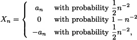
where a₁ = 2 and . Is a martingale?

11.17   Let B_t be a Brownian motion. Find E ((B_t − B_s)⁴).

11.18   Let {B_t; t ≥ 0} and be two independent Brownian motions. Show that

is also a Brownian motion. Find the correlation between B_t and X_t.

11.19   Let B_t be a Brownian motion. Find the distribution of B₁ + B₂ + B₃ + B₄.

11.20   Let {B_t; t ≥ 0} be a Brownian motion. Show that e^−αtB_e^2αt is a Gaussian process. Find its mean and covariance functions.

11.21   Let {B_t; t ≥ 0} be a Brownian motion. Find the distribution for the integral

11.22   S_t has the following differential equations:

dS_t = μS_tdt + σS_tdB_t.

Find the equation for the process .

11.23   Use the Itô formula to write down the stochastic differential equations for the following equations. {B_t; t ≥ 0} is a Brownian motion process.

a) .

b) Y_t = tB_t.

c) Z_t = exp(ct + αB_t).

11.24   Let:

Find E(I_t(B)) and E(I_t(B)²).

11.25   Evaluate the integral

11.26   Evaluate the integral

11.27   Suppose that X_t satisfies:

Let Y_t = f (t, X_t) = (2t + 3)X_t + 4t². Find Y_t.

11.28   Use Itô’s formula to show that:

11.29   Consider the stochastic differential equation

with X₀ = 0.

a) Find X_t.

b) Let Z_t = e^X_t. Find the stochastic differential equation for Z_t using Itô’s formula

11.30   Find the solution of the stochastic differential equation

dZ_t = Z_tdt + 2Z_tdB_t.

11.31   Solve the following stochastic differential equation for the spot rate of interest:

dr_t = (b − r_t)dt + σdB_t

where r_t is an interest rate, and σ ≥ 0.

11.32   Suppose that X_t follows the process dX_t = 0.05X_tdt + 0.25X_tdB_t. Using Itô’s lemma find the equation for process .