CHAPTER 8

LIMIT THEOREMS

The ability to draw conclusions about a population from a given sample and determine how reliable those conclusions are plays a crucial role in statistics. On that account it is essential to study the asymptotic behavior of sequences of random variables. This chapter covers some of the most important results within the limit theorems theory, namely, the weak law of large numbers, the strong law of large numbers, and the central limit theorem, the last one being called so as a way to assert its key role among all the limit theorems in probability theory (see Hernandez and Hernandez, 2003).

8.1   THE WEAK LAW OF LARGE NUMBERS

When the distribution of a random variable X is known, it is usually possible to find its expected value and variance. However, the knowledge of these two quantities do not allow us to find probabilities such as P (|X − c| > ∊) for ∊ > 0. In this regard, the Russian mathematician Chebyschev proved an inequality, appropriately known as Chebyschev’s inequality (compare with exercise 2.48 from Chapter 2), which offers a bound for such probabilities.

Even though in practice it is seldom used, its theoretical importance is unquestionable, as we will see later on.

Chebyschev’s inequality is a particular case of Markov’s inequality (compare with exercise 2.47 from Chapter 2), which we present next.

Lemma 8.1 (Markov’s Inequality) If X is a nonnegative random variable whose expected value exists, then, for all a > 0, we have:

Proof:   Consider the random variable I defined by:

Since X ≥ 0, then , and taking expectations on both sides of this inequality we arrive at the desired expression.          

EXAMPLE 8.1

From past experience, a teacher knows that the score obtained by a student in the final exam of his subject is a random variable with mean 75. Find an upper bound to the probability that the student gets the score greater than or equal to 85.

Solution: Let X be the random variable defined as follows:

X := “Score obtained by the student in the final exam”.

Since X is nonnegative, Markov’s inequality implies that:

P(X ≥ 85) ≤ 0.88235.    

EXAMPLE 8.2

Suppose that X is a random variable having a binomial distribution with parameters 5 and . Use Markov’s inequality to find an upper bound to P(X ≥ 2). Compute P(X ≥ 2) exactly and compare the two results.

Solution: We know that , and therefore, from Markov’s inequality:

On the other hand:

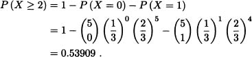
These results show that Markov’s inequality can sometimes give a rather rough estimate of the desired probability.     

In many cases there is no specific information about the distribution of the random variable X and it is in those cases where Chebyschev’s inequality can offer valuable information about the behavior of the random variable.

Theorem 8.1 (Chebyschev’s Inequality) Let X be a random variable such that Var (X) < ∞. Then, for any ∊ > 0, we have:

Proof:   Let Y := |X − E(X)|² and a = ∊². Markov’s inequality yields

which completes the proof.          

Clearly, (8.2) is equivalent to:

Likewise, taking ∊ := σk, with k > 0 and , we obtain:

If in (8.2) E(X) is replaced by a real number C, we obtain:

The above expression is also called “Chebyschev’s inequality” (see Meyer, 1970).

Note 8.1 In (8.1) and (8.2) we can replace P (X ≥ a) and P (|X − E(X)| ≥ ∊) with P (X > a) and P (|X − E(X)| > ∊), respectively, and the inequalities will still hold.

EXAMPLE 8.3

Is there any random variable X for which

where μ_X and σ_X are the expected value and standard deviation of X, respectively?

Solution: It follows from Chebyschev’s inequality that:

Hence, there cannot be a random variable X satisfying (8.3).    

EXAMPLE 8.4

Show that if V ar (X) = 0, then P (X = E(X)) = 1.

Solution: Chebyschev’s inequality implies that for any n ≥ 1:

Taking the limit when n → ∞, we get:

In other words, P (X = E(X)) = 1 .    

The weak law of large numbers can be obtained as an application of Chebyschev’s inequality. This is one of the most important results in probability theory and was initially demonstrated by Jacob Bernoulli for a particular case. The weak law of large numbers states that the expected value E(X) of a random variable X can be considered an “idealization”, for “large enough” n, of the arithmetic mean , where X₁, · · ·, X_n are independent and identically distributed random variables with the same distribution of X.

In order to state this law, we need the following concept:

Definition 8.1 (Identically Distributed Random Variables) X_l, X₂, · · · is said to be a sequence of independent and identically distributed random variables if:

1. For any we have that X₁, · · ·, X_n are independent random variables.

2. For any , X_i and X_j have the same distribution.

Note 8.2 The previous definition can be generalized to random vectors as follows: It is said that X₁, X₂, · · · is a sequence of independent and identically distributed random vectors if:

1. For any we have that X₁, · · · , X_n are independent random vectors.

2. For any , X_i and X_j have the same distribution.

Theorem 8.2 (The Weak Law of Large Numbers (WLLN)) Let X₁, X₂, · · · be a sequence of independent and identically distributed random variables with mean μ and finite variance σ². Then, for any ∊ > 0, we have that

from which we obtain that for any ∊ > 0:

Proof:   Let be the arithmetic mean of the first n random variables. Clearly and V ar . Chebyschev’s inequality implies that for any ∊ > 0 we must have:

which is exactly what we wanted to prove.          

Note 8.3 It is possible to prove the weak law of large numbers without the finite variance hypothesis. That result, due to the Russian mathematician Alexander Khinchin (1894-1959), states the following [see Hernandez (2003) for a proof]:

If X₁, X₂, · · · is sequence of independent and identically distributed random variables with mean μ, then, for any ∊ > 0, we have that:

As a special case of the weak law of large numbers we obtain the following result:

Corollary 8.1 (Bernoulli’s Law of Large Numbers) Let X₁, X₂, · · · be a sequence of independent and identically distributed random variables having a Bernoulli distribution with parameter p. Then, for any ∊ > 0, we have

where K_n := X₁ + · · · + X_n.

Proof:   The weak law of large numbers implies that:

Since p ∈ (0,1), then and consequently (8.4) holds.          

Note 8.4 Bernoulli’s law states that when a random experiment with only two possible results, success or failure, is carried out for a number of times large enough, then, for any ∊ > 0, the set of results for which the proportion of successes is at a distance greater than ∊ of the probability of success p tends to zero. Observe that Bernoulli’s law does not assert that the relative frequency of successes converges to the success probability as the number of repetitions increases. Even when the latter is true, it cannot be directly inferred from Bernoulli’s law.

Note 8.5 Bernoulli’s law was proved by means of the weak law of large numbers, which in turn rests upon Chebyschev’s inequality. However, the original proof given by Bernoulli states that, for arbitrary ∊ > 0 and 0 < δ < 1, we have

where In For example, if ∊ = 0.03 and δ = 0.00002, then n ≥ 12416 implies:

That is, if the experiment is repeated at least 12,416 times, we can be at least 99.998% sure that the success ratio will be less than 3% away from the success probability p.

According to Hernandez (2003), Italian mathematician Francesco Paolo Cantelli (1875−1966) proved an even stronger result, namely, that if n ≥ In then

and thus, for ∊ = 0.03 and δ = 0.00002, n ≥ 42711 implies that:

8.2   CONVERGENCE OF SEQUENCES OF RANDOM VARIABLES

Let X, X₁, X₂, · · · be real-valued random variables all defined over the same probability space. In this section three important and common modes of convergence of the sequence to X will be defined. It is important, however, to clarify that there exist other modes of convergence different from those studied here (in this regard, see, Bauer, 1991).

Definition 8.2 (Convergence in Probability) Let X, X₁, X₂, · · · be realvalued random variables defined over the same probability space . It is said that converges in probability to X and write

if, for any ∊ > 0, the following condition is met:

Note 8.6 Making use of the last definition, we can express the weak law of large numbers as follows: If X₁, X₂, · · · is a sequence of independent and identically distributed random variables with mean μ and finite variance σ², then

where represents the arithmetic mean of the first n random variables.

EXAMPLE 8.5

Let be a sequence of random variables such that and for n = 1,2, · · ·. Let ∊ > 0.

Then:

Therefore:

Thus:

EXAMPLE 8.6

A fair dice is thrown once. For each n = 1,2, · · ·, we define the random variable X_n by

and let X be the random variable given by:

Clearly, for all n = 1,2, · · ·, we have:

|X_n − X| = l.

Hence

and therefore:

A useful result to establish the convergence of a sequence of random variables is the following theorem, whose proof is omitted. We encourage the interested reader to see Jacod and Protter (2004) for a proof.

Theorem 8.3 Let X, X₁, X₂ · · · be real-valued random variables defined over the same probability space . Then if and only if the following expression holds:

Definition 8.3 (Convergence in L^r) Let X, X₁, X₂, · · · be real-valued random variables defined over the same probability space . Let r be a positive integer such that E (|X|^r) < ∞ and E(|X_n|^r) < ∀n. Then if and only if the following expression holds:

EXAMPLE 8.7

Let X₁, X₂, · · · be a sequence of independent and identically distributed random variables with mean μ and finite variance σ². Let

where S_n = X₁ + · · · + X_n. Now:

Hence:

EXAMPLE 8.8

Consider Example 8.5. Since and for n = 1,2, · · ·, we get E(X_n) = 1. Hence, whereas .    

Theorem 8.4 Let r > 0, X, X₁, X₂,· · · be a sequence of random variables such that . This implies .

Proof:   Chebyschev’s inequality implies that for any ∊ > 0 we must have:

Hence, the proof.          

EXAMPLE 8.9

Let where is the Borel σ-algebra on [0,1] and ([0,1]) is the Lebesgue measure on [0,1]. Let

Then for all ∊ > 0:

That is, . But:

Another mode of convergence that will be covered in this section is almost sure convergence, a concept defined below.

Definition 8.4 (Almost Sure Convergence) Let X, X₁, X₂, · · · be real-valued random variables defined over the same probability space . We say that converges almost surely (or with probability 1) to X and write

if the following condition is met:

In other words, if , then:

if and only if p (A) = 1.

EXAMPLE 8.10

Let be an arbitrary probability space and let (X_n)_n be the sequence random variables defined over as follows:

Clearly, for all , we have:

Therefore,

which implies:

8.3   THE STRONG LAW OF LARGE NUMBERS

The following result, known as the strong law of large numbers, states that the average of a sequence of independent and identically distributed random variables converges, with probability 1, to the mean of the distribution.

The proof of this law requires the following lemma [see Jacod and Protter (2004) for a demonstration]:

Lemma 8.2 Let X₁,X₂, · · · be a sequence of random variables. We have that:

1. If all the random variables X_i are positive, then

where the expressions in (8.5) are either both finite or both infinite.

2. If , then converges almost surely and (8.5) holds.

Theorem 8.5 (The Strong Law of Large Numbers (SLLN)) Let X₁,X₂,· · · be a sequence of independent and identically distributed random variables with finite mean μ and finite variance σ². Then:

Proof:   (Jacod and Protter, 2004) Without loss of generality, we can assume that μ = 0.

Since ,

and E (X_jX_k) = 0 for j ≠ k, then (9.7) equals:

Therefore:

Moreover, implies that:

From Lemma 8.2, we have

with probability 1

and consequently lim with probability 1.

Let and k_n be an integer such that:

.

Then

,

so that:

.

Accordingly,

and another application of Lemma 8.2 yields

with probability 1

from which:

with probability 1.

Since lim and , then, with probability 1, we conclude that , which completes the proof for the case μ = 0. If μ ≠ 0, it suffices to consider the random variables defined, for i = 1,2, · · ·, by

Z_i := X_i – μ

and apply the result to the sequence thus obtained.          

The last mode of convergence presented in this text, known as convergence in distribution, is most widely used in applications.

Definition 8.5 (Convergence in Distribution) Let X, X₁, X₂, · · · be realvalued random variables with distribution functions F, F₁, F₂, · · ·, respectively. It is said that converges in distribution to X, written as

if the following condition holds:

for any point x where F is continuous

or, equivalently,

if and only if

for any point x where F is continuous.

Note that convergence in distribution, just like the other modes of convergence previously discussed, reduces itself to the convergence of a sequence of real numbers and not to the convergence of a sequence of events.

EXAMPLE 8.11

Let be a probability space, be the sequence of random variables over defined as

and X = 0. Assume:

we have for each x ≠ 0:

In other words:

Note 8.7 If X, X₁, X₂, · · ·are random variables with values in , then:

X if and only if for all .

The following theorem relates convergence in distribution with convergence of the characteristic functions. Its proof is beyond the scope of this text and the reader may refer to Hernandez (2003) or Rao (1973).

Theorem 8.6 (Lévy and Cramer Continuity Theorem) Let X, X₁, X₂,· · ·be real-valued random variables defined over the same probability space and having the characteristic functions · · · respectively. Then:

if and only if for all .

We proceed now to establish the major links between the convergence modes defined so far, namely, we will see that:

.

Theorem 8.7 Let X, X₁, X₂, · · · be real-valued random variables defined over the same probability space . Then:

.

Proof:   Let ∊ > 0. The sets

form an increasing sequence of events whose union

contains the set

By hypothesis P(A) = 1, from which we infer that P (A_∞) = 1. On the other hand, it follows from the continuity of P that:

Since

and

we conclude that:

Theorem 8.8 Let X, X₁, X₂, · · · be real-valued random variables defined over the same probability space with distribution functions F, F₁, F₂, · · · respectively. Then:

.

Proof:   Let x be a point of continuity of F. We need to prove that . Since F is continuous at x, then, for any ∊ > 0, there exists a δ > 0 0 such that:

.

On the other hand, since , then there exists such that, for n ≥ n (∊), the following condition is satisfied:

.

Furthermore, we have that:

.

Analogously:

.

Figure 8.1   Relationship between the different modes of convergence

Thus:

That is, for all n ≥ n(), we have that

and consequently:

Note 8.8 The converse of the above theorem is not, in general, true. Consider, for example, the random variables given in Example 8.6. In that case, we have , but .

Figure 8.1 summarizes the relationship between the different modes of convergence. In this figure, the dotted arrow means that the convergence in probability does not imply the convergence in almost surely. However, we can prove that there is a subsequence of the original sequence that converges almost surely.

All the definitions given so far can be generalized to random vectors in the following way:

Definition 8.6 (Convergence of Random Vectors) Let X, X₁, X₂, · · · be k-dimensional random vectors, , having the distribution functions F_x, F_x1, F_x2, · · ·, respectively. Then, it is said that:

1. converges in probability to X, written as , if the ith component of X_n converges in probability to the ith component of X. for each i = 1,2, · · ·, k.

2. converges almost surely (or with probability 1) to X, written as , if the ith component of X_n converges almost surely to the ith component of X for each i = 1, 2, · · ·, k.

3. converges in distribution to X, written as , if lim_{n → ∞}F_Xn(x) = F_X(x) for all points of continuity of F_X (·).

8.4   CENTRAL LIMIT THEOREM

This section is devoted to one of the most important results in probability theory, the central limit theorem, whose earliest version was first proved in 1733 by the French mathematician Abraham DeMoivre. In 1812 Pierre Simon Laplace, also a French mathematician, proved a more general version of the theorem. The version known nowadays was proved in 1901 by the Russian mathematician Liapounoff.

The central limit theorem states that the sum of independent and identically distributed random variables has, approximately, a normal distribution whenever the number of random variables is large enough and their variance is finite and different from zero.

Theorem 8.9 (Univariate Central Limit Theorem (CLT)) Let X₁, X₂, · · · be a sequence of independent and identically distributed random variables with mean μ and finite variance σ². Let and Y_n := . Then, the sequence of random variables Y₁, Y₂, · · · converges in distribution to a random variable Y having a standard normal distribution. In other words:

Proof:   Without loss of generality, it will be assumed that μ = 0. Let be the characteristic function of the random variables X₁, X₂, · · ·. Since the random variables are independent and identically distributed, we have that:

Expansion of in a Taylor series about zero yields:

Thus:

Taking the limit when n → ∞ we get:

The Lévy-Cramer continuity theorem implies that

where Y is a random variable having a standard normal distribution.         

Note 8.9 The de Moivre-Laplace theorem (4.6) is a particular case of the central limit theorem. Indeed, if X₁, X₂, · · · are independent and identically distributed random variables having a Bernoulli distribution of parameter p, then the conditions given in (8.9) are satisfied.

Note 8.10 Let X₁, X₂, · · · be a sequence of independent and identically distributed random variables with mean μ and finite positive variance σ². The central limit theorem asserts that, for large enough n, the random variable has, approximately, a normal distribution with parameters nμ and nσ².

Note 8.11 The central limit theorem can be applied to most of the classic distributions, namely: binomial, Poisson, negative binomial, gamma, Weibull, etc., since all of them satisfy the hypotheses required by the theorem. However, it cannot be applied to Cauchy distribution since it does not meet the requirements of the central limit theorem.

Note 8.12 There are many generalizations of the central limit theorem, among which the Lindenberg-Feller theorem stands out in that it allows for the sequence X₁, X₂, · · · of independent random variables with different means E(X_i) = μ_i and different variances .

Note 8.13 (Multivariate Central Limit Theorem) The central limit theorem can be generalized to sequences of random variables as follows:

Let X₁, X₂, · · · be a sequence of k-dimensional independent and identically distributed random vectors, with , having mean vector μ and variance- covariance matrix , where is positive definite. Let

be the vector of arithmetic means. Then

where X is a k-dimensional random vector having a multivariate normal distribution with mean vector 0 and variance-covariance matrix . (See Hernandez, 2003).

Some applications of the central limit theorem are given in the examples below.

EXAMPLE 8.12

A fair dice is tossed 1000 times. Find the probability that the number 4 appears at least 150 times.

Solution: Let X := “Number of times that the number 4 is obtained”. We know that . Applying the de Moivre-Laplace theorem, we can approximate this distribution with a normal distribution of mean and variance . Therefore:

EXAMPLE 8.13

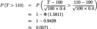
Suppose that for any student the time required for a teacher to grade the final exams of his probability course is a random variable with mean 1 hour and standard deviation 0.4 hours. If there are 100 students in the course, what is the probability that he needs more than 110 hours to grade the exam?

Solution: Let X_i be the random variable representing the time required by the teacher to grade the ith student of his course. We need to calculate the probability that greater than 110. By the central limit theorem, we have:

EXAMPLE 8.14

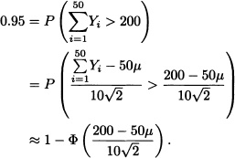
(Wackerly et al., 2008) Many raw materials, like iron ore, coal and unrefined sugar, are sampled to determine their quality by taking small periodic samples of the material as it moves over a conveyor belt. Later on, the small samples are gathered and mixed into a compound sample which is then submitted for analysis. Let Y_i be the volume of the ith small sample in a particular lot, and assume that Y₁, Y₂, · · ·, Y_n is a random sample where each Y_i has mean μ (in cubic inches) and variance σ². The average volume of the samples can be adjusted by changing the settings of the sampling equipment. Suppose that the variance σ² of the volume of the samples is approximately 4. The analysis of the compound sample requires that, with a 0.95 probability, n = 50 small samples give rise to a compound sample of 200 cubic inches. Determine how the average sample volume μ must be set in order to meet this last requirement.

Solution: The random variables Y₁, Y₂, · · ·, Y₅₀ are independent and identically distributed having mean μ and variance σ² = 4. By the central limit theorem, has, approximately, a normal distribution with mean 50μ and variance 200. We wish to find μ such that = 0.95. Accordingly:

That is,

which in turn implies

from which we obtain:

EXERCISES

8.1   Suppose that 50 electronic components say D₁, D₂, · · ·, D₅₀, are used in the following manner. As soon as D₁ fails, D₂ becomes operative. When D₂ fails, D₃ becomes operative, etc. Assume that the time to failure of D_i is an exponentially distributed random variable with parameter 0.05 per hour. Let T be the total time of operation of the 50 devices. Compute the approximate probability that T exceeds 500 hours using the central limit theorem?

8.2   Let X₁, X₂, · · ·, X_n be n independent Poisson distributed random variables with means 1,2, · · ·, n, respectively. Find an x in terms of t such that

for sufficiently large n

where is the cdf of (0,1).

8.3   Suppose that X_i, i = 1,2, · · ·, 450, are independent random variables each having a distribution (0,1). Evaluate approximately.

8.4   Let Y   be a gamma distributed random variable with pdf

Find the limiting distribution of as p → ∞.

8.5   Let . Use the CLT to find n such that:

P[X > n/2] ≥ 1 − α.

Calculate the value of n when α = 0.90 and p = 0.45.

8.6   A fair coin is flipped 100 consecutive times. Let X be the number of heads obtained. Use Chebyschev’s inequality to find a lower bound for the probability that differs from by less than 0.1.

8.7   Let X₁, X₂ · · ·, X₅₀ be independent and identically distributed random variables having a Poisson distribution with mean 2.5. Compute:

8.8   (ChernofF Bounds) Suppose that the moment generating function m_X(t) of a random variable X exists. Use Markov’s inequality to show that for any the following holds:

a) P(X ≥ a) ≤ exp(−ta) m_X(t) for all t > 0.

b) P(X ≤ a) ≤ exp(−ta) m_X(t) for all t < 0.

8.9   (Jensen Inequality) Let f be a twice-differentiable convex real-valued function, that is, f″ (x) ≥ 0 for all x. Prove that if X is a real-valued random variable, then

E(f(X)) ≥ f(E(X))

subject to the existence of the expected values.

Hint: Consider the Taylor polynomial of f about μ = E(X).

8.10   If X is a nonnegative random variable with mean 2, what can be said about E(X³) and E(In X).

8.11   Let X, X₁, X₂, · · · be real-valued random variables defined over the same probability space . Show the following properties about convergence in probability:

a) if and only if .

b) If and , then P(X = Y) = 1.

c) If , then .

d) If and , then .

e) If and k is a real constant, then .

f) If and , then .

8.12   Let X, X₁, X₂, · · · be real-valued random variables defined over the same probability space . Prove that:

a) If and , then .

b) If and , then .

8.13   Let f be a continuous real-valued function and let X, X₁, X₂, · · · be real-valued random variables over the same probability space . Show that if , then .

Note: The result still holds if almost sure convergence is replaced by convergence in probability.

8.14   Let X, X₁, X₂, · · · be real-valued random variables defined over the same probability space . Show that if , where k is a real constant, then .

8.15   Suppose that a Bernoulli sequence has length equal to 100 with a success probability of p = 0.7. Let X := “Number of successes obtained”. Compute P(X ∈ [65,80]).

8.16   A certain medicine has been shown to produce allergic reactions in 1% of the population. If this medicine is dispensed to 500 people, what is the probability that at most 10 of them show any allergy symptoms?

8.17   A fair dice is rolled as many times as needed until the sum of all the results obtained is greater than 200. What is the probability that at least 50 tosses are needed?

8.18   A Colombian coffee exporter reports that the amount of impurities in 1 pound of coffee is a random variable with mean 3.4 mg and standard deviation 4 mg. In a sample of 100 pounds of coffee from this exporter, what is the probability that the sample mean is greater than 4.5 mg?

8.19   (Ross, 1998) Let X be a random variable having a gamma distribution with parameters n and 1. How large must n be in order to guarantee that:

8.20   How many tosses of a fair coin are needed so that the probability that the average number of heads obtained differs at most 0.01 from 0.5 is at least 0.90?

8.21   Let X be a nonnegative random variable. Prove:

8.22   Let (X_n)_n≥1 be a sequence of random variables, and let c be a real constant verifying, for any ∊ > 0, the following condition:

Prove that for any bounded continuous function g we have that:

8.23   Examine the nature of convergence of {X_n} defined below for the different values of k for n = 1,2, · · · :

8.24   Show that the convergence in the rth mean does not imply almost sure convergence for the sequence {X_n} defined below:

8.25   Use CLT to show that .

8.26   Let be a sequence of random variables such that . Show that .

8.27   For each n ≥ 1, let X_n be an uniformly distributed random variable over set , that is:

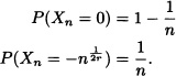
Let U be a random variable with uniform distribution in the interval [0,1]. Show that .

8.28   Let be a sequence of i.i.d. random variables with E(X₁) = V ar(X₁) = ∈ (0, ∞) and P(X₁ > 0) = 1. Show that, for n → ∞ ,

where:

8.29   Let be a sequence of random variables such that . Show that .

8.30   Let . Prove the following statements:

a) If is a sequence of random variables with , then with .

b) The sequence with converges in distribution but does not converge in probability to .

8.31   Let be a sequence of i.i.d. random variables with P(X_n = 1) = P(X_n = −1) = . Show that

converges in probability to 0.