CHAPTER 7

MULTIVARIATE NORMAL DISTRIBUTIONS

The multivariate normal distributions is one of the most important multidimensional distributions and is essential to multivariate statistics. The multivariate normal distribution is an extension of the univariate normal distribution and shares many of its features. This distribution can be completely described by its means, variances and covariances given in this chapter. The brief introduction to this distribution given will be necessary for students who wish to take the next course in multivariate statistics but can be skipped otherwise.

7.1   MULTIVARIATE NORMAL DISTRIBUTION

Definition 7.1 (Multivariate Normal Distribution) An n-dimensional random vector X = (X₁, …, X_n) is said to have a multivariate normal distribution if any linear combination has a univariate normal distribution (possibly degenerated, as happens, for example, when α_j = 0 for all j).

  EXAMPLE 7.1

Suppose that X₁, …, X_n are n independent random variables such that

for j = 1, …, n. Then, if , we have

where

In other words,

Therefore, the vector X : = (X₁, …, X_n) has a multivariate normal distribution.    

Note 7.1 In this chapter, the vector in is represented by a row vector.

Theorem 7.1 Let X : = (X₁,…, X_n) be a random vector. X has multivariate normal distribution if and only if its characteristic function has the form

where , Σ is a positive semidefinite symmetric square matrix and •, • represents the usual inner product of .

Proof:

and

where α := (α₁, …, α_n) and Σ is the variance-covariance matrix of X.

Therefore, the characteristic function of Y equals:

Then:

The characteristic function of Y is then given by

where β := tα. That is:

Then Y has a univariate normal distribution with parameters α,μ and α, αΣ. Therefore, X is multivariate normal.        

Note 7.2 It can be easily verified that the vector μ and the matrix Σ from the previous theorem correspond to the expected value and the variance-covariance matrix of X, respectively.

Notation 7.1 if X has a multivariate normal distribution with mean vector μ and variance-covariance matrix Σ, then we write .

Our next theorem states that any multivariate normal distribution can be obtained by applying a linear transformation to a random vector whose components are independent random variables having all univariate normal distributions. In order to prove this result, the following lemma is required:

Lemma 7.1 Let X : = (X₁,…,X_n) be a random vector such that (μ,Σ). The components X_j, j = 1, …, n, are independent if and only if the matrix Σ is diagonal.

Proof:

See the result given in (5.17).

Suppose that the matrix Σ is diagonal. Since , then:

Therefore, the random variables X_j for j = 1, …, n, are independent.      

Theorem 7.2 Let X := (X₁,…,X_n) be a random vector such that X (μ,Σ). Then there exist an orthogonal matrix A and independent random variables Y₁, …, Y_n such that either Y_j = 0 or for j = 1, …, n so that X = μ + YA.

Proof: Since Σ is a positive semidefinite symmetric matrix, there exist a diagonal matrix Λ whose entries are all nonnegative and an orthogonal matrix A such that:

Let Y := (X − μ)A^T. Since X is multivariate normal, so is Y. Additionally, Λ is the variance-covariance matrix of Y. Since this matrix is diagonal, it follows from the previous lemma that the components of Y are independent. Finally we have:

Suppose that X = (X₁, …, X_n) is an n-dimensional random vector and that the random variables X₁, …, X_n are independent and identically distributed having a standard normal distribution. The joint probability density function of X₁, …, X_n is given by:

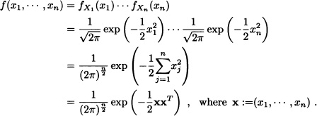
In addition, it is clear that the vector X has a multivariate normal distribution. The natural question that arises is: If X is a random vector with multivariate normal distribution, under what conditions can the existence of a density function for the vector X be guaranteed? The answer is given in the following theorem:

Theorem 7.3 Let . If Σ is a positive definite matrix, then X has a density function given by:

Proof:   Since Σ is a positive definite matrix, all its eigenvalues are positive. Moreover, there exists an orthogonal matrix U such that

where Λ = diag(λ_i) and λ₁, …, λ_n are the eigenvalues of Σ. In other words, Λ is the diagonal matrix whose entries on the diagonal are precisely the eigen-values of Σ.

Let A := U diagU^T. Clearly A^TA = Σ and A is also a positive definite matrix. Let h : R^l×n → R^l×n be defined by h(x) = xA + μ. The inverse function of h would then be given by h⁻¹(x) = (x − μ)A^−l. The transformation theorem implies that the density function of X := YA + μ, where Y = (Y₁,…,Y_n), is an n-dimensional random vector such that the random variables Y₁, …, Y_n are independent and identically distributed with a standard normal distribution and is given by:

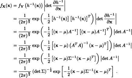
Note 7.3 (Bivariate Normal Distribution) As a particular case of the theorem above, suppose that

where

and

with ρ representing the correlation coefficient. Therefore:

Since

and

we obtain:

We also have that:

In other words, the marginal distributions of X = (X₁,X₂) are univariate normal.

In general, we have:

Theorem 7.4 All the marginal distributions of are multivariate normal

Proof: Suppose that X = (X₁, …, X_n) and let

where {k₁, …, k_l} is a subset of {1, …, n). The characteristic function of is given by:

Therefore has a multivariate normal distribution.

7.2   DISTRIBUTION OF QUADRATIC FORMS OF MULTIVARIATE NORMAL VECTORS

Let X_i, i = 1,2, …, n be independent normal random variables with , i = 1,2,…,n. It is known that:

Suppose now an n-dimensional random vector X = (X₁, X₂, …, X_n) having multivariate normal distribution with mean vector μ and variance and covariance matrix Σ. Suppose that Σ is a positive definite matrix. From Theorem 7.3, it is known that X has the density function given by

with . Now we are interested in finding the distribution of W = . In order to do so, we need to find the moment generating function of W. We have:

This last integral exists for all values of t < .

Now the matrix (1 − 2t)Σ⁻¹, t < , is positive definite given that Σ is also a positive definite matrix.

On the other hand,

and consequently the function

is the density function of the multivariate normal random variable. When multiplying and dividing the denominator by (1 − 2t)^n/2 in the expression given for m(t) we obtain

which corresponds to the mgf of a random variables with distribution.

We also have that .

Suppose that X₁, X₂, …, X_n are independent with normal distribution (0,σ²). Let X = (X₁, X₂, …, X_n) and suppose that A is a real symmetric matrix of order n. We want to find the distribution of XAX^T. In order to find this distribution, the mgf of the variable must be considered. It is clear that:

Given that the random variables X₁, X₂, … X_n are independent with normal distribution (0,σ²), we have in this case that

where I_n is the identity matrix of order n.

Therefore:

Given that I − 2tA is a positive definite matrix and if |t| is sufficiently small, let’s say |t| < h, we have that the function

is the density function of the multivariate normal distribution. Thus:

Suppose now that λ₁,λ₂,…, λ_n are eigenvalues of A and let L be an orthogonal matrix of order n such that L^TAL = diag(λ₁, λ₂, …, λ_n). Then

and therefore:

Given that

and because L is an orthogonal matrix, we have

from which we obtain that:

Suppose that r is the rank of matrix A with 0 < r ≤ n. Then we have that exactly r of the numbers λ₁, λ₂, …, λ_n, let’s say λ₁, …, λ_r, are different from zero and the remaining n − r of them are zero. Therefore:

Under which conditions does the previous mgf correspond to the mgf of a random variable with chi-squared distribution of k degrees of freedom? If this is to be so, then we must have:

This implies (1 − 2tλ₁) · · · (1 − 2tλ_r) = (1 − 2t)^k and in consequence k = r and λ₁ = λ₂ = · · · = λ_r = 1. That is, matrix A has r eigenvalues equal to 1 and the other n − r equal to zero, and the rank of the matrix A is r. This implies that matrix A must be idempotent,that is, A² = A.

Conversely, if matrix A has rank r and is idempotent, then A has r eigenvalues equal to 1 and n − r real eigenvalues equal to zero and in consequence the mgf of is given by:

In summary:

Theorem 7.5 Let X₁,X₂,… X_n be i.i.d. random variables with (0,σ²). Let X = (X₁, X₂, …, X_n) and A be a symmetric matrix of order n with rank r. Suppose that Y := XAX^T. Then:

  EXAMPLE 7.2

Let Y = X₁X₂ − X₃X₄ where X₁, X₂, X₃, X₄ are i.i.d. random variables with (0,σ²). Is the distribution of the random variable a chi-square distribution? Explain.

Solution: It is clear that Y = XAX^T with:

The random variable does not have distribution because A² ≠ A.

Suppose that X₁,X₂, …, X_n are i.i.d. random variables with (0,σ²). Let A and B be two symmetric matrices of order n and consider the quadratic forms XAX^T and XBX^T. Under what conditions are these quadratic forms independent? To answer this question we must consider the joint mgf of and We have then:

In this case, we have that det Σ = σ²ⁿ and . So that:

The matrix I − 2t₁A − 2t₂B is a positive definite matrix if |t₁| and |t₂| are sufficiently small, for example, |t₁| < h₁ and |t₂| < h₂ with h₁, h₂ > 0. Hence:

If XAX^T and XBX^T are stochastically independent, then AB = 0. Indeed, if XAX^T and XBX^T are independent, then m(t₁,t₂) = m(t₁,0) · (0,t₂) for all t₁,t₂ with |t₁| < h₁ and |t₂| < h₂. That is,

where t₁,t₂ satisfy |t₁| < h₁ and |t₂| < h₂.

Let r = rank(A) and suppose that λ₁, λ₂,…, λ_r are r eigenvalues of A different than zero. Then there exists an orthogonal matrix L such that:

Suppose that Then, the equation

may be rewritten as

or equivalently:

That is:

Given that the coefficient of (−2t₁)^r on the right side of the previous equation is λ₁λ₂ … λ_rdet(I − 2t₂D) and the coefficient of (−2t₁)^r on the left side of the equation is

where I_n−1 is the (n − r)-order identity matrix, then, for all t₂ with |t₂| < h₂, det(I − 2t₂D) = det(I_n−r − 2t₂D₂₂) must be satisfied and consequently the nonzero eigenvalues of the matrices D and D₂₂ are equal.

On the other hand, if A = (a_ij)_n×n is a symmetric matrix, then is equal to the sum of the squares of the eigenvalues of A. Indeed, let L be such that L^TAL = diag(λ₁, λ₂, …, λ_n). Then:

Therefore, the sum of the squares of the elements of matrix D is equal to the sum of the squares of the elements of matrix D₂₂. Thus:

Now 0 = CD = L^TAL · L^TBL = L^T ABL and in consequence AB = 0.

Suppose now that AB = 0. Let us verify that and are stochastically independent. We have that:

That is:

Therefore:

In summary, we have the following result:

Theorem 7.6 Let X₁,X₂,…, X_n - i.i.d. random variables with (0,σ²). Let A and B be symmetric matrices and X = (X₁, X₂, … X_n). Then, the quadratic forms XAX^T and XBX^T are independent if and only if AB = 0.

EXERCISES

7.1   Let X = (X, Y) be a random vector having a bivariate normal distribution with parameters μX = 2, μY = 3.1, σX = 0.001, σY = 0.02 and ρ = 0. Find:

7.2   Suppose that X₁ and X₂ are independent (0,1) random variables. Let Y₁ = X₁ + 3X₂ − 2 and Y₂ = X₁ − 2X₂ + 1. Determine the distribution of Y = (Y₁,Y₂).

7.3   Let X = (X₁, X₂) be a multivariate normal with μ = (5,10) and Σ = . If Y₁ = 2X₁ + 2X₂ + 1 and Y₂ = 3X₁ − 2X₂ − 2 are independent, determine the value of α.

7.4   Let X = (X₁, …, X_n) be an n-dimensional random vector such that , where Σ is a nonsingular matrix. Prove that

is a random vector with a (0,1) distribution, where I is the identity matrix of order n and W is a matrix satisfying W² = Σ. In this case, we say that the vector Y has a standard multivariate normal distribution.

7.5   Let X = (X, Y) be a random vector with bivariate normal distribution. Prove that the conditional distribution of Y, given that X = x, is normal with parameters μ given by

and σ² given by

7.6   Let X = (X₁,X₂) be multivariate normal with μ = (1,−1) and Σ = . Let Y_l = X₁ − X₂ − 2 and Y₂ = X₁+ X₂.

a) Find the distribution of Y = (Y₁,Y₂).

b) Find the density function fY (y₁,y₂).

7.7   Suppose that X is multivariate normal (μ,Σ) where μ = 1 and:

Find the conditional distribution of X₁ + X₂ given X₁ − X₂ =0.

7.8   Let X = (X₁, X₂, X₃) be a random vector with normal multivariate distribution of parameters μ = 0 and Σ given by:

Find P (X₁ > 0, X₂ > 0, X₃ > 0).

7.9   Let X = (X₁,X₂,X₃) be a random vector with normal multivariate distribution of parameters μ = 0 and Σ given by:

Find the density function f (x₁, x₂, x₃) of X.

7.10   The random vector X has three-dimensional normal distribution with mean vector 0 and covariance matrix Σ given by:

Find the distribution of X₂ given that X₁ − X₃ = 1 and X₂ + X₃ = 0.

7.11   The random vector X has three-dimensional normal distribution with expectation 0 and covariance matrix Σ given by:

Find the distribution of X₃ given that X₁ = 1.

7.12   The random vector X has three-dimensional normal distribution with expectation 0 and covariance matrix Σ given by:

Find the distribution of X₂ given that X₁ + X₃ = 1.

7.13   Let , where:

Determine the conditional distribution of X₁ − X₃ given that X₂ = −1.

7.14   The random vector X has three-dimensional normal distribution with mean vector μ and covariance matrix Σ given by:

Find the conditional distribution of X₁ given that X₁ = −X₂.

7.15   The random vector X has three-dimensional normal distribution with expectation 0 and covariance matrix Σ given by:

Find the distribution of X₂ given that X₁ = X₂ = X₃.