CHAPTER 6

CONDITIONAL EXPECTATION

One of the most important and useful concepts of probability theory is the conditional expected value. The reason for it is twofold: in the first place, in practice usually it is interesting to calculate probabilities and expected values when some partial information is already known. On the other hand, when one wants to find a probability or an expected value, many times it is convenient to condition first with respect to an appropriate random variable.

6.1   CONDITIONAL DISTRIBUTION

The relationship between two random variables can be seen by finding the conditional distribution of one of them given the value of the other. In Chapter 1, we defined the conditional probability of an event A given another event B as:

It is natural, then, to have the following definition:

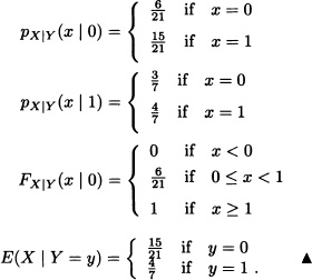
Definition 6.1  (Conditional Probability Mass Function) Let X and Y be two discrete random variables. The conditional probability mass functio of X given Y = y is defined as

for all y for which P (Y = y) > 0.

Definition 6.2  (Conditional Distribution Function) The conditional distribution function of X given Y = y is defined as

for all y for which P (Y = y) > 0.

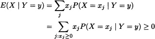
Definition 6.3  (Conditional Expectation) The conditional expectation of X given Y = y is defined as:

The quantity E(X | Y = y) is called the regression of X on Y = y.

  EXAMPLE 6.1

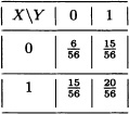
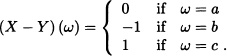
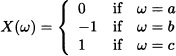
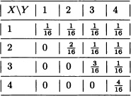
A box contains five red balls and three green ones. A random sample of size 2 (without replacement) is drawn from the box. Let:

The joint probability distribution of the random variables X and Y is given by:

Hence:

  EXAMPLE 6.2

Let X and Y be independent Poisson random variables with parameters λ₁ and λ₂, respectively. Calculate the expected value of X under the condition that X + Y = n, where n is a nonnegative fixed integer.

Solution: Let:

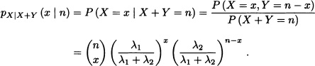
That is, X has, under the condition X + Y = n, a binomial distribution with parameters n and Therefore:

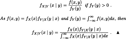
Definition 6.4  (Conditional Probability Density Function) Let X and Y be continuous random variables with joint probability density function f. The conditional probability density function of X given Y = y is defined as

for all y with f_Y(y) > 0.

Definition 6.5  (Conditional Distribution Function) The conditional distribution function of X given Y = y is defined as

for all y with f_Y(y) > 0.

Definition 6.6  (Conditional Expectation) The conditional expectation of X given Y = y is defined as

for all y with f_Y(y) > 0.

  EXAMPLE 6.3

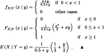
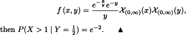
Let X and Y be random variables with joint probability density function given by:

For 0 < y < 1 we can obtain that:

  EXAMPLE 6.4

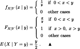
Let X and Y be random variables with joint probability density function given by

where λ > 0. For y > 0 we obtain:

  EXAMPLE 6.5

Let X and Y be random variables with joint probability density function given by:

Calculate f_XY (x | y) and E(X | Y = y).

Solution: The marginal density function of Y is equal to:

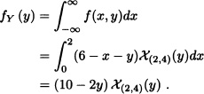
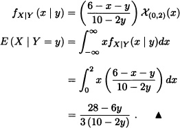
Then, for 2 < y < 4, we obtain that:

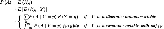
Note 6.1 For all y, with f_Y (y) > 0 and all Borel set A in , it can be said that:

  EXAMPLE 6.6

If X and Y are random variables with joint probability density function given by

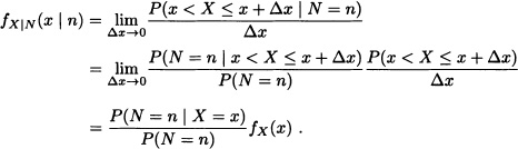
Note 6.2 If X and Y are independent random variables, then the conditional density of X given Y = y is equal to the density of X.

Note 6.3 (Bayes’ Rule)

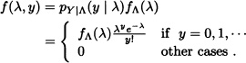
So far we have defined the conditional distributions when both the random variables under consideration are either discrete or continuous. Suppose now that X is an absolutely continuous random variable and that N is a discrete random variable. In this case:

  EXAMPLE 6.7

Let X be a random variable with uniform distribution over the interval (0,1) and N, a binomial random variable with parameters n + m and X. Then, for 0 < x < 1, we have that

where . That is, under the condition N = n, X has a beta distribution with parameters n + 1 and m + 1.     

  EXAMPLE 6.8

Let Y be a Poisson random variable with parameter Λ, where the parameter Λ itself is distributed as Γ(α,β). Calculate f_Λ|Y(λ | y).

Solution: It is known that:

Then:

Given that:

it is obtained that:

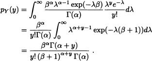
Consequently, for λ > 0 and y a nonnegative integer:

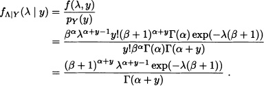
That is, under the condition Y = y, Λ has a gamma distribution with parameters α + y and β + 1.     

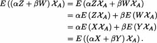
Definition 6.7  Let X and Y be real random variables and h a real function such that h(X) is a random variable. Define

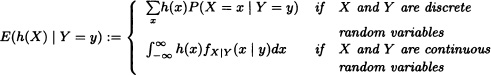
for all values y of Y for which P(Y = y) > 0 in the discrete case and f_y(y) > 0 in the continuous case.

  EXAMPLE 6.9

Let X and Y be random variables with joint probability density function given by:

We have that:

Therefore, for y > 0, we have:

Now, it can be deduced that:

From the previous definition, a new random variable can be defined as follows:

Definition 6.8  (Conditional Expectation) Let X and Y be real random variables defined over and h a real-valued function such that h(X) is a random variable. The random variable E(h(X) | Y) defined by

is called the conditional expected value of h(X) given Y.

  EXAMPLE 6.10

Let .

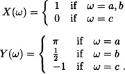
     Consider the random variables X and Y defined as follows:

Then:

It is obtained that:

In the same way, it can be verified that:

Then:

It may be observed, additionally, that:

The above result of the example is proved in the following theorem in a general setup.

Theorem 6.1 Let X ,Y be real random variables defined over and h a real-valued function such that h(X) is a random variable. If E(h(X)) exists, then:

E(h(X)) = E(E(h(X)) | Y).

Proof:  Suppose that X and Y are discrete random variables. Then:

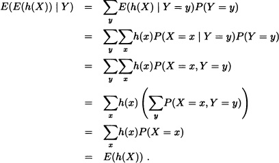
If X and Y are random variables with joint probability density function f, then:

          

  EXAMPLE 6.11

The number of clients who arrive at a store in a day is a Poisson random variable with mean λ = 10. The amount of money (in thousands of pesos) spent by each client is a random variable with uniform distribution over the interval (0,100]. Determine the amount of money that the store is expecting to collect in a day.

Solution: Let X and M be random variables defined by:

X := “Number of clients who arrive at the store in a day”.

M := “Amount of money that the store collects in a day”.

It is clear that

where:

M_i := “Amount of money spent by the ith client”.

According to the previous theorem, it can be obtained that:

E(M) = E(E(M | X)).

Give:

Then:

E(M) = E(50X) = 50E(X) = 500,000 pesos.      

Note 6.4 In particular it is said that, if is an arbitrary probability space and if is fixed, then:

  EXAMPLE 6.12

Let X and Y be independent random variables with densities f_X and f_y, respectively. Calculate P(X < Y).

Solution: Let A := {X < Y}. Then

where F_X(.) is the distribution function of X.     

Theorem 6.2 If X, Y and Z are real random variables defined over and if h is a real function such that h(y) is a random variable, then the conditional expected value satisfies the following conditions:

1. E(X | Y) ≥ 0 if X ≥ 0 a.s.

2. E(1 | Y) = 1.

3. If X and Y are independent, then E(X | Y) = E(X).

4. E(Xh(y) | Y) = h(y)E(X | Y).

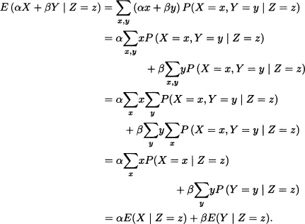
5. E(αX + βY | Z)= αE(X | Z) + βE(Y | Z) for .

Proof:  We present the proof for the discrete case. Proof for the continuous case can be obtained in a similar way.

1. Suppose that X takes the values x₁, x₂, …. Given that P(X < 0) = 0, then P(X = x_j) = 0 for x_j < 0. Therefore,

and in consequence E(X | Y) ≥ 0.

2. Let X := 1. Then:

E(X | Y = y) = 1P(X = 1 | Y = y) = 1.

3. As X and Y are independent, it is obtained that

P(X = x | Y = y) = P(X = x)

for all y with P(Y = y) > 0. Therefore:

4.

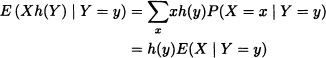
and we have:

E(Xh(Y) | Y) = h(Y)E(X | Y).

5.

Therefore:

E(αX + βY | Z) = αE(X | Z) + βE(Y | Z).

          

  EXAMPLE 6.13

Consider the n + m Bernoulli trials, each trial with success probability p. Calculate the expected number of success in the first n attempts.

Solution: Let Y :=“total number of successes” and, for each i = 1, …, n, let:

It is clear that:

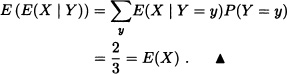
As

E(X) = E(E(X | Y))

and

then:

  EXAMPLE 6.14

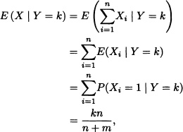
The number of customers entering a supermarket in a given hour is a random variable with mean 100 and standard deviation 20. Each customer, independently of the others, spends a random amount of money with mean $100 and standard deviation $50. Find the mean and standard deviation of the amount of money spent during the hour.

Solution: Let N be the number of customers entering the supermarket. Let X_i be the amount spent by the ith customer. Then the total amount of money spent is . The mean is:

Using

Var(X) = E(Var(X | Y)) + Var(E(X|Y))

we get:

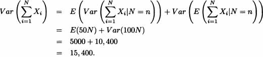
Hence the standard deviation is 124.0967.     

  EXAMPLE 6.15

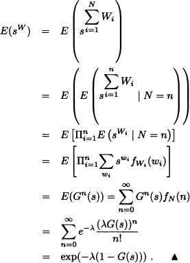
A hen lays N eggs, where N has a Poisson distribution with mean λ. The weight of the nth egg is W_n, where W₁, W₂, … are independent and identically distributed random variables with common probability generating function G. Prove that the probability generating function of the total weight W_i is exp(−λ(1 − G(s))).

Solution: The pgf of the total weight is:

6.2   CONDITIONAL EXPECTATION GIVEN A σ-ALGEBRA

In this section the concept of conditional expected value of a random variable with respect to a σ-algebra will be worked which generalizes the concept of conditional expected value developed in the previous section.

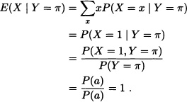
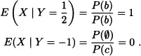
Definition 6.9  (Conditional Expectation of X Given B) Let X be a real random variable defined over and let with P(B) > 0. The conditional expected value of X given B is defined as

if the expected value of exists.

  EXAMPLE 6.16

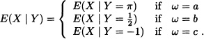
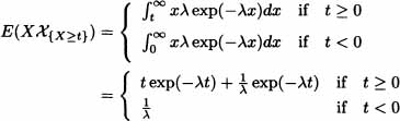
A fair die is thrown twice consecutively. Let X be a random variable that denotes the sum of the results obtained and B be the event that indicates that the first throw is 5. Calculate E(X | B).

Solution: The sample space of the experiment is given by:

It is clear that:

Then

and

Therefore:

  EXAMPLE 6.17

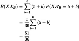
Let X be a random variable with exponential distribution with parameter λ. Calculate E(X | {X ≥ t}).

Solution: Given that we have that the density function is given by:

Therefore:

On the other hand,

and we obtain:

  EXAMPLE 6.18

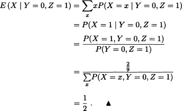
Let X, Y and Z be random variables with joint distribution given by:

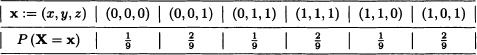
Calculate E(X | Y = 0, Z = 1).

Solution:

Definition 6.10  (Conditional Expectation of X Given ) Let X be a real random variable defined over for which E(X) exists. Let be a sub-σ-algebra of . The conditional expected value of X given , denoted by E(X | ), is a random variable -measurable so that:

  EXAMPLE 6.19

Let and for all . Suppose that X is a real random variable given by

and let .

We have Y given by

which is equal to E(X | ). Indeed:

1. Y is -measurable, due to the fact that:

2. Y satisfies condition (6.1) because:

Therefore,

and we obtain:

  EXAMPLE 6.20

Let and for all . Suppose that X is a real random variable given by

and let .

It is easy to verify that Z := 0 is -measurable and that it satisfies condition (6.1). Therefore, Z = E(X | ).     

Definition 6.11  We define:

L₁ := {X : X is a real random variable defined over and with E (|X|) < ∞}.

In continuation we present some important properties of conditional expectation with respect to a σ-algebra:

Theorem 6.3 Let be a sub-σ-algebra of . We have:

1. If X,Y L₁ and , then E (αX + βY) = αE (X) + βE (y).

2. If X is -measurable and in L₁, then E (X | ) = X. In particular, E(c | ) = c for all c real constant.

3. .

4. If X ≤ 0 and X L₁, then E (X | ) ≥ 0.

5. If X, Y L₁ and X ≤ Y, then E (X | ) ≤ E (Y | ).

6. If , then for all X L₁ we have that:

7. If X L₁, then |E(X | )| ≤ E(|X| | ).

Proof:

1. Since Z = E(X | ) and W = E(Y | ) are -measurable, then αZ + βW are also -measurable. From the definition of the conditional expectation, we have that for all :

2. By the hypothesis X is -measurable, and from the definition of conditional expectation, if Z ≔ E(X | ), then for all :

3. It is clear that Z = E(X) is measurable with respect to . On the other hand, if we have that .

4. Let Z = E (X | ). By the definition, we have that, for all ,

since because of Z ≥ 0.

5. This result follows from the linearity of expectation and the previous result. It is clear that is -measurable. Let and . If , then:

Since , then , and it follows that:

Therefore, for all :

That is,

and we get:

Similarly, if and , then for all it is true that:

Since , we have:

Because of this, for all we have:

Thus:

In particular, if , then .

6. Let X⁺ and X⁻ be the positive and negative parts of X, respectively. That is:

Because

we have:

          

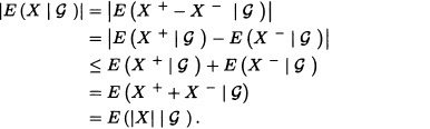
Finally we have the following property whose proof is beyond the scope of this text. Interested readers may refer to Jacod and Protter (2004).

Theorem 6.4 Let be a probability space and let be a sub-σ-algebra of . If X L₁ and (X_n)_n≥1 is an increasing sequence of nonnegative real random variables defined over Ω that converges to X a.s., that is,

then (E(X_n | ))_n≥1 is an increasing sequence of random variables that converges to E(X | ).

Theorem 6.5 Let be a probability space and let be a sub-σ-algebra of . If (X_n)_n≥1 is a sequence of real random variables in L₁ that converge in probability to 1 and if |X_n| ≤ Z for all n, where Z is a random variable in L₁, then:

Notation 6.1 Let X, Y₁, … , Y_n be the real random variables. The expectation E(X | σ(Y₁, … , Y_n)), where σ(Y₁, … , Y_n) is the smallest σ-algebra with respect to random variables Y₁, … ,Y_n, is usually denoted by E(X | Y₁, … , Y_n).

Note 6.5 Conditional expectation is a very useful application in Bayesian theory of statistics. A classic problem in this theory is obtained when observing data X ≔ (X₁, … , X_n) whose distribution is determined from the conditional distribution of X given ⊖ = , where ⊖ is considered as a random variable with a specific priori distribution. Using as a base the value of the data X, the interesting problem is to estimate the unknown value of . An estimator of can be any function d(X) of the data. In Bayesian theory we look for choosing d(X) in such a way that the conditional expected value of the square of the distance between the estimator and the parameter is minimized. In other words we look for minimizing E([ – d(X)]² | X).

Conditioning on X leaves us with a constant d(X). Along with this and the fact that for any random variable W we have that E[(W – c)²] is minimized when c = E(W), we conclude that the estimator minimizing E([ – d(X)]² | X) is given by d(X) = E ( | X). This estimator is called the Bayes estimator.

  EXAMPLE 6.21

The height reached by the son of an individual with a height of x cm is a random variable with normal distribution with mean x + 3 and variance 2. Which is the best prediction of the height that is expected for the son of the individual with height 170 cm?

Solution: let X be the random variable that denotes the height of the father and let be the random variable that denotes the height of the son. According to the information provided, . Due to the previous observation, it is known that the best possible predictor of the son’s height is d(X) = E ( | X). Therefore, if X = 170, then and:

EXERCISES

6.1  Consider a sequence of Bernoulli trials. If the probability of success is a random variable with uniform distribution in the interval (0,1), what is the probability that n trials are needed?

6.2  Let X be a random variable with uniform distribution over the interval (0,1) and let Y be a random variable with uniform distribution over (0, X). Determine:

a)  The joint probability density function of X and Y.

b)  The marginal density function of Y.

6.3  Let Y be a random variable with Poisson distribution with parameter λ. Suppose that Z is a random variable defined by

where the random variables X₁, X₂, … are mutually independent and independent of Y. Further, suppose that the random variables X₁,X₂, … are identically distributed with Bernoulli distribution with parameter p (0,1). Find E(Z) and Var (Z).

6.4  Let X and Y be random variables uniformly distributed over the triangular region limited by x = 2, y = 0 and 2y = x, that is, the joint density function of the random variables X and Y is given by:

Calculate:

a) .

b) P(Y ≥ 0.5).

c) P(X ≤ 1.5 | Y = 0.5).

6.5  The joint density function of X and Y is given by:

Find the conditional density function of X given that Y = y and the conditional density function for Y given that X = x.

6.6  Let X = (X, Y) be a random vector with density function given by:

Calculate:

a) The marginal density functions of X and Y.

b) The conditional density function f_y|x (y | X = 2).

c) The value of c so that P(Y > c | X = 2) = 0.05.

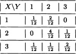
6.7  Suppose that X and Y are discrete random variables with joint probability distribution given by:

a) Calculate distributions of X and Y.

b) Determine E(X | Y = 1) and E(Y | X = 1).

6.8  Suppose that X and Y are discrete random variables with joint probability distribution given by:

Verify that E (E (X | Y)) = E(X) and E (E (Y | X)) = E(Y).

6.9  A fair die is tossed twice consecutively. Let X be a random variable that denotes the number of even numbers obtained and Y the random variable that denotes the number of results obtained that are less than 4. Find E(XE(Y | X)).

6.10  If E[Y/X) = 1, show that:

6.11  A box contains 8 red balls and 5 black ones. Two consecutive extractions are done without replacement. In the first extraction 2 balls are taken out while in the second extraction 3 balls are taken out. Let X be the random variable that denotes the number of red balls taken out in the first extraction and Y the random variable that denotes the number of red balls taken out in the second extraction. Find E (Y | X = 1).

6.12  A player extracts 2 balls, one after the other one, from a box that contains 5 red balls and 4 black ones. For each red ball extracted the player wins two monetary units, and for each black ball extracted the player loses one monetary unit. Let X be a variable that denotes the player’s fortune and Y be a random variable that takes the value 1 if the first ball extracted is red and the value 0 if the first ball extracted is black.

a) Calculate E (X | Y).

b) Use part (a) to find E(X).

6.13  Assume that taxis are waiting in a queue for passengers to come. Passengers for these taxis arrive independently with interarrival times that are exponentially distributed with mean 1 minute. A taxi departs as soon as two passengers have been collected or 3 minutes have expired since the first passenger has got in the taxi. Suppose you get in the taxi as the first passenger. What is your average waiting time for the departure?

6.14 Suppose you are in Ooty, India, as a tourist and lost at a point with five roads. Out of them, two roads bring you back to the same point after 1 hour of walk. The other two roads bring you back to the same point after 3 hours of travel. The last road leads to the center of the city after 2 hours of walk. Assume that there are no road sign. Assume that you choose a road equally likely at all times independent of earlier choices. What is the mean time until you arrive at the city?

6.15  Suppose that X is a discrete random variable with probability mass function given by , x = 1,2 and Y is a random variable such that:

Find:

a) The joint distribution of X and Y.

b) E(X | Y).

6.16  If X has a Bernoulli distribution with parameter p and E (Y | X = 0) = 1 and E (Y | X = 1) = 2, what is E(Y)?

6.17  Suppose that the joint probability density function of the random variables X and Y is given by:

a) Calculate P(X > 2 | Y < 4).

b) Calculate E(X | Y = y).

c) Calculate E(Y | X = x).

d) Verify that E(X) = E(E(X | Y)) and E(Y) = E(E(Y | X)).

6.18  Let X and Y be independent random variables. Prove that:

E(Y | X = x) = E(Y) for all x.

6.19  Prove that if E(Y | X = x) = E(Y) for all x, then X and Y are noncorrelated. Give a counterexample that shows the reciprocal is not true.

Suggestion: You can use the fact that E(XY) = E(XE(Y | X)).

6.20  Let X and Y be random variables with joint probability density function given by:

Calculate .

6.21  The conditional variance of Y given X = x is defined by:

Var(Y | X = x) := E(Y² | X = x) – (E(Y | X = x))².

Prove that:

Var(Y) = E(Var(Y | X)) + Var(E(Y | X)).

6.22  Let X and Y be random variables with joint distribution given by:

Find Var(Y | X).

6.23  Let X and Y be random variables with joint probability density function given by:

Calculate E(X | Y = 1).

6.24  Let (X, Y) be two-dimensional random variables with joint pdf given by:

a) Find the conditional distribution of Y given X = x.

b) Find the regression of Y on X.

c) Show that variance of Y for given X = x does not involve x.

6.25  Suppose that the joint probability density function of the random variables X and Y is given by:

Calculate E(X | Y = y).

6.26  Let (X, Y) be a random vector with uniform distribution in a triangle limited by x ≥ 0, y ≥ 0 and x + y ≤ 2. Calculate E(Y | X = x).

6.27  Let X and Y be random variables with joint probability density function given by:

Calculate:

a) E(X | Y = y).

b) E(X² | Y = y).

c) Var(X | Y = y).

6.28  Two fair dice are tossed simultaneously. Let X be the random variable that denotes the sum of the results obtained and B the event defined by B :=“the sum of the results obtained is divisible by 3”. Calculate E(X | B).

6.29  Let X and Y be i.i.d. random variables each with uniform distribution over the interval (0,2). Calculate:

a) P(X ≥ 1 | (X + Y) ≤ 3).

b) E(X | (X + Y) ≤ 3).

6.30  Let X and Y be random variables with joint density function given by:

Calculate E(X + Y | X < Y).

6.31  A fair die is thrown in a successive way. Let X and Y be random variables that denote, respectively, the number of throws required to obtain 2 and 4. Calculate:

a) E(X).

b) E(X | Y = 1).

c) E(X | Y = 5).

6.32  A box contains 6 red balls and 5 white ones. Two samples are extracted in a consecutive way without replacement of sizes 3 and 5. Let X be the number of white balls in the first sample and Y the number of white balls in the second sample. Calculate E(X | Y = k) for k = 1,2,3,4,5.

6.33  Let X be a random variable whose expected value exists. Prove that:

E(X) = E(X | X < y)P(X < y) + E(X | X ≥ y)P(X ≥ y).

6.34  The conditional covariance of X and Y given Z is defined by:

Cov(X, Y | Z) := E[(X – E(X | Z))(Y – E(Y | Z)) | Z].

a) Prove that:

Cov(X, Y | Z) = E(XY | Z) – E(X | Z)E(Y | Z).

b) Verify that:

Cov(X,Y) = E[Cov(X,Y | Z)] + Cov(E[X | Z],E[Y | Z)).

6.35  Let X₁ and X₂ be a two i.i.d. random variables each (0,1) distributed.

a) Are X₁ + X₂ and X₁ – X₂ independent random variables? Justify your answers.

b) Obtain .

6.36  Let (X, Y) be two-dimensional random variable with joint pdf

a) Compute E[(2X + 1) | Y = y].

b) Find the standard deviation of [X | Y = y].

6.37  For n ≥ 1, let , … be i.i.d. random variables with values in . Suppose that and . Let Z₀ := 1 and:

a) Calculate E(Z_n+1 | Z_n) and E(Z_n).

b) Let with |s| ≤ 1, the probability generating function of Z₁ . Calculate f_n(s) := E(s^Z_n) in terms of f.

c) Find Var(Z_n).