
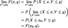
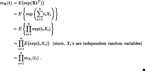
CHAPTER 5
RANDOM VECTORS
In the previous chapters, we have been concentrating on a random variable defined in an experiment, e.g., the number of heads obtained when three coins are tossed. In other words, we have been discussing the random variables but one at a time. In this chapter, we learn how to treat two random variables, of both the discrete as well as the continuous types, simultaneously in order to understand the interdependence between them. For instance, in a telephone exchange, the time of a call arrival X and a call duration Y or the shock arrivals X and the consequent damage Y are of interest. One of the questions which also comes to mind is, can we relate two random variables defined on the same sample space, or in other words, can two random variables of the same spaces be correlated? Some of these questions will be discussed and answered in this chapter.
5.1 JOINT DISTRIBUTION OF RANDOM VARIABLES
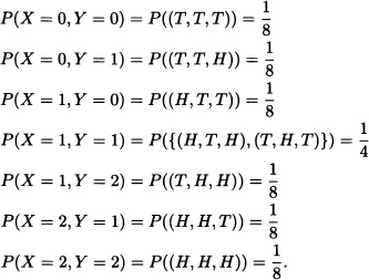
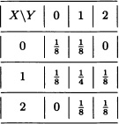
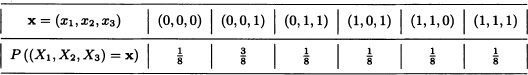
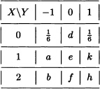
In many cases it is necessary to consider the joint behavior of two or more random variables. Suppose, for example, that a fair coin is flipped three consecutive times and we wish to analyze the joint behavior of the random variables X and Y defined as follows:
X := “Number of heads obtained in the first two flips”.
Y := “Number of heads obtained in the last two flips”.
Clearly:
This information can be summarized in the following table:
Definition 5.1 (n-Dimensional Random Vector) Let X1, X2, · · ·, Xn be n real random variables defined over the same probability space (Ω, ![]() , P). The function
, P). The function ![]() defined by
defined by
![]()
is called an n-dimensional random vector.
Definition 5.2 (Distribution of a Random Vector) Let X be an n-dimensional random vector. The probability measure defined by
![]()
is called the distribution of the random vector X.
Definition 5.3 (Joint Probability Mass Function) Let X = (X1, X2, · · ·, Xn) be an n-dimensional random vector. If the random variables Xi, with i = 1, · · ·, n, are all discrete, it is said that the random vector X is discrete. In this case, the probability mass function of X, also called the joint distribution function of the random variables X1, X2, · · ·, Xn, is defined by:
![]()
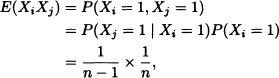
Note 5.1 Let X1 and X2 be discrete random variables. Then:
In general, we have:
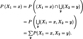
Theorem 5.1 Let X = (X1, X2, · · ·, Xn) be a discrete n-dimensional random vector. Then, for all j = 1, · · ·, n we have:
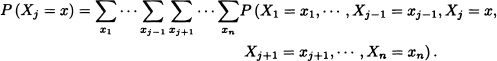
The function
![]()
is called the marginal distribution of the random variable Xj.
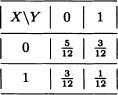
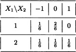
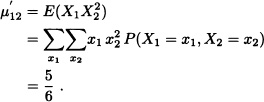
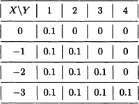
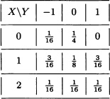
Let X and Y be discrete random variables with joint distribution given by:
The marginal distributions of X and Y are given, respectively, by:
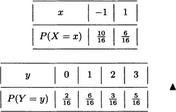
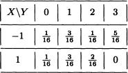
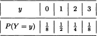
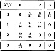
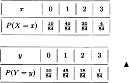
Suppose that a fair coin is flipped three consecutive times and let X and Y be the random variables defined as follows:
X := “Number of heads obtained”.
Y := “Flip number where a head was first obtained” (if there are none, we define Y = 0).
- Find the joint distribution of X and Y.
- Calculate the marginal distributions of X and Y.
- Calculate P(X ≤ 2, Y = 1), P(X ≤ 2, Y ≤ 1) and P(X ≤ 2 or Y ≤ 1).
Solution:
- The joint distribution of X and Y is given by:
- The marginal distributions of X and Y are presented in the following tables:
- It follows from the previous items that:
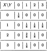
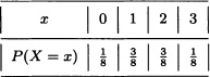
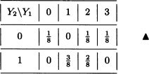
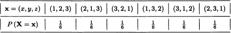
A box contains three nails, four drawing-pins and two screws. Three objects are randomly extracted without replacement. Let X and Y be the number of drawing-pins and nails, respectively, in the sample. Find the joint distribution of X and Y.
Solution: Since
![]()
the joint distribution of the variables X and Y is given by:
The marginal distributions of X and Y are, respectively:
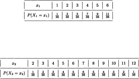
A fair dice is rolled twice in a row. Let:
X1 := “Greatest value obtained”.
X2 := “Sum of the results obtained”.
The density function of the random vector X = (X1, X2) is given by:
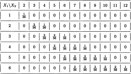
The marginal distributions of X1 and X2 are, respectively:
Furthermore, we have that
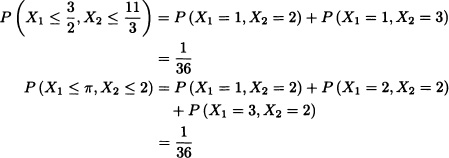
and in general:
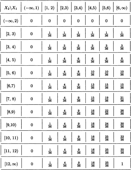
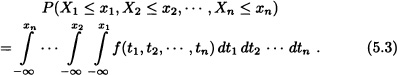
Each entry in the table represents the probability that
P(X1 ≤ x1, X2 ≤ x2)
for the values x1 and x2 indicated in the first row and column, respectively. ![]()
The previous example leads us to the following definition:
Definition 5.4 (Joint Cumulative Distribution Function) Let X = (X1, X2, · · ·, Xn) be an n-dimensional random vector. The function defined by
F(x1, x2, · · ·, xn) := P(X1 ≤ x1, X2 ≤ x2, · · ·, Xn ≤ xn),
for all ![]() is called the joint cumulative distribution function of the random variables X1, X2, · · ·, Xn, or simply the distribution function of the n-dimensional random vector X.
is called the joint cumulative distribution function of the random variables X1, X2, · · ·, Xn, or simply the distribution function of the n-dimensional random vector X.
Note 5.2 Just like the one-dimensional case, we have that the distribution of the random vector X is completely determined by its distribution function.
Note 5.3 Let X1 and X2 be random variables with joint cumulative distribution function F. Then:
Likewise, we have that ![]() . This can be generalized in the following theorem:
. This can be generalized in the following theorem:
Theorem 5.2 Let X = (X1, X2, · · ·, Xn) be an n-dimensional random vector with joint cumulative distribution function F. For each j = 1, · · ·, n, the cumulative distribution function of the random variable Xj is given by:
![]()
The distribution function FXj is called the marginal cumulative distribution function of the random variable Xj.
The previous theorem shows that if the cumulative distribution function of the random variables X1, · · ·, Xn, is known, then the marginal distributions are also known. The converse however does not always hold.
Next we present some of the properties of the joint distribution function.
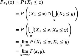
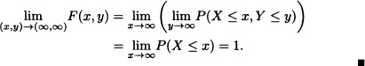
Theorem 5.3 Let X = (X, Y) be a two-dimensional random vector. The joint cumulative distribution function F of the random variables X, Y has the following properties:
1.
3.
![]()
4.
![]()
Proof:
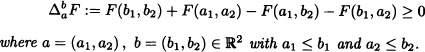
- Let a = (a1, a2), b = (b1, b2) with a1 < b1, a2 < b2 and:
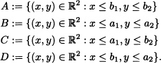
If I := (A − C) − (D − B), then, clearly:
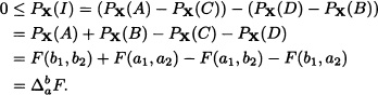
- We prove (5.1) and leave (5.2) as an exercise for the reader:
- Since
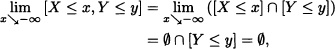
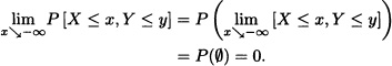
Analogously, we can verify that:
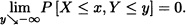
- It is straightforward that:
The following theorem is the general case for n-dimensional random vectors of the above theorem which can be proved in a similar fashion.
Theorem 5.4 Let X = (X1, X2, · · ·, Xn) be an n-dimensional random vector. The joint cumulative distribution function F of the random variables X1, X2, · · ·, Xn has the following properties:
1. ![]() for all
for all ![]() with a ≤ b, where:
with a ≤ b, where:

2. F is right continuous on each component.
3. For all ![]() with i = 1, · · ·, n, we have:
with i = 1, · · ·, n, we have:
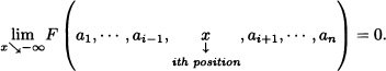
4.
![]()
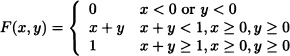
Check whether the following functions are joint cumulative distribution functions:
Solution:
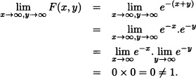
F(x, y) is not a joint cumulative distribution function.
- For instance, take
 .
.
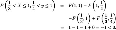
F(x, y) is not a joint cumulative distribution function.
- For instance, take

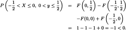
F(x, y) is not a joint cumulative distribution function.
- Since all the four properties of Theorem 5.3 are satisfied, F(x, y) is a joint cumulative distribution function.

Definition 5.5 (Jointly Continuous Random Variables) Let X1, X2, · · ·, Xn be n real-valued random variables defined over the same probability space. It is said that the random variables are jointly continuous, if there is an integrable function ![]() such that for every Borel set C of
such that for every Borel set C of ![]() :
:
![]()
The function f is called the joint probability density function of the random variables X1, X2, · · ·, Xn.
Note 5.4 From the definition above, we have, in particular:
1. ![]()
2.
The previous remark shows that if the joint probability density function f of the random variables X1, X2, · · ·, Xn is known, then the joint distribution function F is also known. This raises the question: Does the converse hold as well? That is, is it possible, starting with the joint distribution function F, to find the joint probability density function f? The answer is given in the next theorem:
Theorem 5.5 Let X and Y be continuous random variables having a joint distribution function F. Then, the joint probability density function f is
![]()
for all the points (x, y) where f(x, y) is continuous.
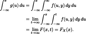
Proof: By applying the fundamental theorem of calculus to (5.3), we obtain
![]()
and therefore:
![]()
Since ![]() and
and ![]() exist and are both continuous, then
exist and are both continuous, then
![]()
which completes the proof of the theorem. ![]()
Furthermore, if X1, · · ·, Xn are n continuous random variables with joint distribution function F, then the function g(·, · · ·, ·) defined over ![]() by
by
is a joint probability density function of the random variables X1, · · ·, Xn.
Suppose now that X and Y are continuous random variables having joint probability density function f, and let g be the function defined by:
![]()
Clearly:
Moreover, since
![]()
g is the density function of the random variable X called the marginal density function of X and is commonly notated as fX(x).
![]()
is the density function of the random variable Y.
In general, we have the following result:
Theorem 5.6 If X1, X2, · · ·, Xn are n real-valued random variables, having joint pdf f, then
![]()
is the density function of the random variable Xj for j = 1, 2, · · ·, n.
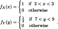
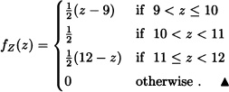
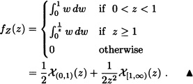
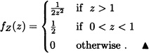
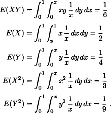
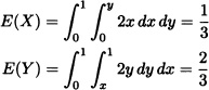
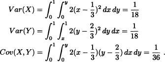
Let X and Y be random variables with joint pdf given by:
![]()
- Calculate
 .
. - Compute
 .
.
Solution:
Let X and Y be random variables with joint pdf given by:
![]()
- Calculate
 .
. - Find the marginal density functions of X and Y.
Solution:
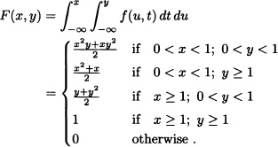
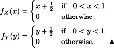
Let X and Y be random variables with joint probability density function given by:
![]()
Find:
- The joint cumulative distribution function of X and Y.
- The marginal density functions of X and Y.
Solution:
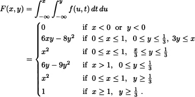
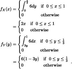
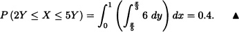
Let X and Y be random variables with joint probability density function given by:
![]()
- The value of the constant k.
- The joint cumulative distribution function of X and Y.
- The marginal density functions of X and Y.
- P(2Y ≤ X ≤ 5Y).
Solution:
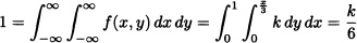
so that k = 6.
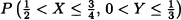
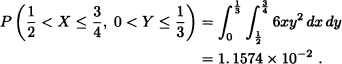
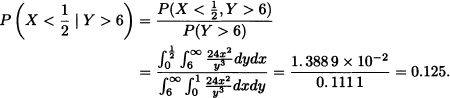
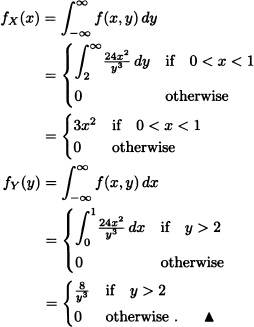
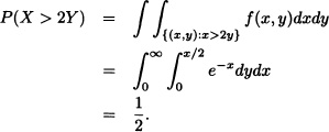
The system analyst at an email server in a university is interested in the joint behavior of the random variable X, defined as the total time between an email’s arrival at the server and departure from the service window, and Y, the time an email waits in the buffer before reaching the service window. Because X includes the time an email waits in the buffer, we must have X > Y. The relative frequency distribution of observed values of X and Y can be modeled by the joint pdf
![]()
with time measured in seconds.
- Find P(X < 2, Y > 1).
- Find P(X > 2Y).
- Find P(X – Y ≥ 1).
Solution:
5.2 INDEPENDENT RANDOM VARIABLES
Definition 5.6 (Independent Random Variables) Let X and Y be two real-valued random variables defined over the same probability space. If for any pair of Borel sets A and B of ![]() we have
we have
![]()
then X and Y are said to be independent.
We say that X and Y are independent and identically distributed (i.i.d.) random variablesif X and Y are independent random variables and have the same distributions.
Note 5.5 (Independent Random Vectors) The previous definition can be generalized to random vectors as follows: Two n-dimensional random vectors X and Y defined over the same probability space (Ω, ![]() , P) are said to be independent, if for any A and B Borel subsets of
, P) are said to be independent, if for any A and B Borel subsets of ![]() they satisfy:
they satisfy:
![]()
Assume that X and Y are independent random variables. Then it follows from the definition above that:
![]()
That is:
Conversely, if the condition (5.4) is met, then the random variables are independent.
Suppose now that X and Y are independent discrete random variables. Then
for all x in the image of X and all y in the image of Y. Conversely, if the condition (5.5) is met, then, the random variables are independent.
If X and Y are independent random variables with joint density function f(x, y), then:
P(x < X ≤ x+dx, y < Y ≤ y+dy) = P(x < X ≤ x+dx)P(y < Y ≤ y+dy).
That is:
Conversely, if the condition (5.6) is satisfied, then the random variables are independent. In conclusion, we have that the random variables X and Y are independent if and only if its joint density function f(x, y) can be factorized as the product of their marginal density functions fX(x) and fY(y).
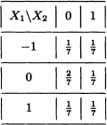
There are nine colored balls inside an urn, three of which are red while the remaining six are blue. A random sample of size 2 (with replacement) is extracted. Let X and Y be the random variables defined by:
Are X and Y independent? Explain.
Solution: The joint distribution function of X and Y is given by:
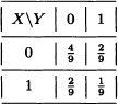
It can be easily verified that for any choice of x, y ![]() {0, 1}:
{0, 1}:
P(X = x, Y = y) = P(X = x)P(Y = y).
That is, X and Y are independent random variables, which was to be expected since the composition of the urn is the same for each extraction. ![]()
Solve the previous exercise, now under the assumption that the extraction takes place without replacement.
Solution: In this case, the joint distribution function of X and Y is given by:
Given:
![]()
Then X and Y are not independent. ![]()
Let X and Y be independent random variables with density functions given by:
Find P(XY > 1).
Solution: Since X and Y are independent, their joint density function is given by:
![]()
Accordingly:
![]()
Note 5.6 Let X and Y be independent discrete random variables with values in ![]() . Clearly:
. Clearly:
Suppose that X and Y are independent random variables with ![]() and
and ![]() . Find the distribution of Z = X + Y.
. Find the distribution of Z = X + Y.
Solution: The random variables X and Y take the values 0, 1, · · ·, and therefore the random variable Z also takes the values 0, 1, · · ·. Let z ![]() {0, 1, · · ·}. Then:
{0, 1, · · ·}. Then:
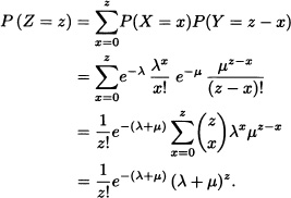
That is, ![]() .
. ![]()
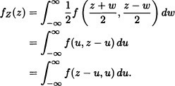
Note 5.7 Suppose that X and Y are independent random variables having joint probability density function f(x, y) and marginal density functions fX and fY, respectively. The distribution function of the random variable Z = X + Y can be obtained as follows:

Upon derivation, equation (5.7) yields the density function of the random variable Z as follows:

The density function of the random variable Z is called the convolution of the density functions fX and fY and is notated fX * fY.
Let X and Y be i.i.d. random variables having an exponential distribution of parameter λ > 0. The density function of Z = X + Y is given by:
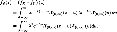
Given:
![]()
Then :
That is, ![]() .
. ![]()
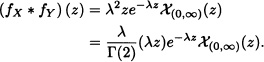
Let X and Y be independent random variables such that ![]() and
and ![]() . Calculate P(X + Y ≥ 1).
. Calculate P(X + Y ≥ 1).
Solution: The joint probability density function of X and Y is given by
![]()
so that:
Below, the notion of independence is generalized to n random variables:
Definition 5.7 (Independence of n Random Variables) n real-valued random variables X1, X2, · · ·, Xn defined over the same probability space are called independent if and only if for any collection of Borel subsets A1, A2, · · ·, An of ![]() the following condition holds:
the following condition holds:
![]()
Note 5.8 (Independence of n Random Vectors) The definition above can be extended to random vectors in the following way: n k-dimensional random vectors X1, X2, · · ·, Xn, defined over the same probability space (Ω, ![]() , P), are said to be independent if and only if they satisfy
, P), are said to be independent if and only if they satisfy
![]()
for any collection of Borel subsets A1, A2, · · ·, An of ![]() .
.
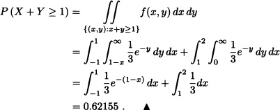
![]() EXAMPLE 5.17 Distribution of the Maximum and Minimum
EXAMPLE 5.17 Distribution of the Maximum and Minimum
Let X1, · · ·, Xn be n real-valued random variables defined over (Ω, ![]() , P) and consider the random variables Y and Z defined as follows:
, P) and consider the random variables Y and Z defined as follows:
![]()
and
![]()
Clearly,
FY(y) := P(Y ≤ y) = P(X1 ≤ y, · · ·, Xn ≤ y)
and:
FZ(z) := P(Z ≤ z) = 1 – P(X1 > z, · · ·, Xn > z).
Therefore, if the random variables X1, · · ·, Xn are independent, then
where FXk (·) is the distribution function of the random variable Xk for k = 1, · · ·, n. ![]()
Let X and Y be independent and identically distributed random variables having an exponential distribution of parameter a. Determine the density function of the random variable Z := max{X, Y3}.
Solution: The density function of the random variable U = Y3 is given by:
![]()
Since the random variables X and Y3 are independent, it follows from the previous example that Z = max{X, Y3} has the following cumulative distribution function:
FZ(z) = FX(z)FY3(z).
Therefore, the density function of Z is given by:
fZ(z) = fX(z)FY3(z) + FX(z)fY3(z).
That is:
![]()
Note 5.9 If X1, X2, · · ·, Xn are n independent random variables, then X1, X2, · · ·, Xk with k ≤ n are also independent. To this effect, let A1, A2, · · ·, Ak be Borel subsets of ![]() . Then:
. Then:
Suppose that X1, X2 and X3 are independent discrete random variables and let Y1 := X1 + X2 and ![]() . Then:
. Then:
That is, Y1 := X1 + X2 and ![]() are independent random variables. Does this result hold in general? The answer to this question is given by the following theorem whose demonstration is omitted since it relies on measuretheoretic results.
are independent random variables. Does this result hold in general? The answer to this question is given by the following theorem whose demonstration is omitted since it relies on measuretheoretic results.
Theorem 5.7 Let X1, · · ·, Xn, be n independent random variables. Let Y be a random variable defined in terms of X1, · · ·, Xk and let Z be a random variable defined in terms of Xk+1, · · ·, Xn, where 1 ≤ k < n. Then Y and Z are independent.
Let X1, · · ·, X5 be independent random variables. By Theorem 5.7, it is obvious that Y = X1X2 + X3 and Z = eX5 sin X4 are independent random variables. ![]()
5.3 DISTRIBUTION OF FUNCTIONS OF A RANDOM VECTOR
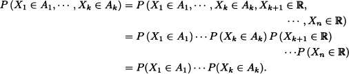
Let X = (X1, X2, · · ·, Xn) be a random vector and let g1(·, · · ·, ·), · · ·, gk(·, · · ·, ·) be real-valued functions defined over ![]() . Consider the following random variables: Y1 := g1(X1, · · ·, Xn), · · ·, Yk := gk(X1, · · ·, Xn). We wish to determine the joint distribution of Y1, · · ·, Yk in terms of the joint distribution of the random variables X1, · · ·, Xn.
. Consider the following random variables: Y1 := g1(X1, · · ·, Xn), · · ·, Yk := gk(X1, · · ·, Xn). We wish to determine the joint distribution of Y1, · · ·, Yk in terms of the joint distribution of the random variables X1, · · ·, Xn.
Suppose that the random variables X1, · · ·, Xn are discrete and that their joint distribution is known. Clearly:
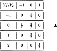
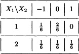
Let X1 and X2 be random variables with joint distribution given by:
Let g1(x1, x2) := x1 + x2 and g2(x1, x2) = x1x2. Clearly, the random variables
Y1 := g1(X1, X2) = X1 + X2 and Y2 := g2(X1, X2) = X1X2
take, respectively, the values –1, 0, 1, 2 and –1, 0, 1. The joint distribution of Y1 and Y2 is given by:
Let X1, X2 and X3 be random variables having joint distribution function given by:
Let g1(x1, x2, x3) := x1 + x2 + x3, g2(x1, x2, x3) = |x3 − x2|. The joint distribution of Y1 := g1(X1, X2, X3) and Y2 := g2(X1, X2, X3) is given by:
In the case of absolutely continuous random variables, we have the following result. The interested reader can consult its proof in Jacod and Protter (2004).
Theorem 5.8 (Transformation Theorem) Let X = (X1, X2, · · ·, Xn) be a random vector with joint density function fX. Let ![]() be an injective map. Suppose that both g and its inverse
be an injective map. Suppose that both g and its inverse ![]() are continuous. If the partial derivatives of h exist and are continuous and if their Jacobian J is different from zero, then the random vector Y := g(X) has joint density function fY given by:
are continuous. If the partial derivatives of h exist and are continuous and if their Jacobian J is different from zero, then the random vector Y := g(X) has joint density function fY given by:
![]()
Let X = (X1, X2) be a random vector having joint probability density function given by:
![]()
Find the joint probability density function of Y = (Y1, Y2), where Y1 = X1 + X2 and Y2 = X1 − X2.
Solution: In this case we have
g(x1, x2) = (g1(x1, x2), g2(x1, x2)) = (x1 + x2, x1 − x2)
and the inverse transformation is given by:
![]()
The Jacobian J of the inverse transformation would then equal:
![]()
Therefore, the joint probability density function of Y is:
![]()
In general we have the following result for distribution of the sum and the difference of random variables.
Theorem 5.9 Let X and Y be random variables having joint probability density function f. Let Z := X + Y and W := X – Y. Then the probability density functions of Z and W are given by
![]()
![]()
respectively.
Proof: Just like in the previous example, we have that
g(x, y) := (x + y, x − y)
and the inverse transformation h is given by:
![]()
Therefore, the joint probability density function of Z and W equals
![]()
from which we obtain that:
In a similar fashion:
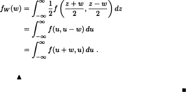
Note 5.10 In the particular case where the random variables X and Y are independent, the density function of the random variable Z := X + Y is given by
where fX(·) and fY(·) represent the density functions of X and Y respectively. The expression given in (5.9) is the convolution of fX and fY, notated as fX * fY [compare with (5.8)].
Let X and Y be independent random variables having density functions given by:
Determine the density function of Z = X + Y.
Solution: We know that:
![]()
Since
![]()
we obtain:
Let X and Y be random variables having the joint probability density function given by:
![]()
Find the density function of W := X – Y.
Solution: According to Theorem 5.9:
![]()
Here:
![]()
![]()
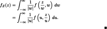
Theorem 5.10 (Distribution of the Product of Random Variables) Let X and Y be random variables having joint probability density function f. Let Z := XY. Then the density function of Z is given by:
![]()
Proof: We introduce W := Y. Let g be the function defined by:
g(x, y) := (g1(x, y), g2(x, y)) = (xy, y).
The inverse transformation equals:
![]()
The Jacobian of the inverse transformation is:
![]()
Therefore, the joint probability density function of Z and W is given by:
![]()
Now, we obtain the following expression for the density function of Z = XY:
Let X and Y be two independent and identically distributed random variables, having uniform distribution on the interval (0, 1). According to the previous example, the density function of Z := XY is given by
where fX and fY represent the density functions of X and Y respectively. Since
![]()
then:
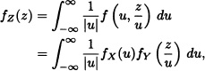
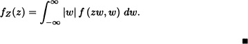
Theorem 5.11 (Distribution of the Quotient of Random Variables) Let X and Y be random variables having joint probability density function f. Let ![]() [which is well defined if P(Y = 0) = 0)]. Then the density function of Z is given by:
[which is well defined if P(Y = 0) = 0)]. Then the density function of Z is given by:
![]()
Proof: We introduce W := Y. Now, consider the function
![]()
The inverse transformation is then given by:
h(x, y) = (xy, y).
Its Jacobian equals:
![]()
Then the joint density function of Z and W is given by:
fZW(z, w) = |w|f (zw, w).
Therefore, a density function of Z is:
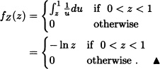
Let X and Y be two independent and identically distributed random variables having uniform distribution on the interval (0, 1). According to the previous example, the density function of ![]() is given by
is given by
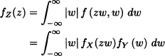
where fX and fY represent the density functions of X and Y, respectively. Since
![]()
then:
Assume that the lifetime X of an electric device is a continuous random variable having a probability density function given by:
![]()
Let X1 and X2 be the life spans of two independent devices. Find the density function of the random variable ![]() .
.
Solution: It is known that:
![]()
Since
![]()
(i) If z ≥ 1, then f(υz)f(υ) does not equal zero if and only if υ > 1000. Thus:
![]()
(ii) If 0 < z < 1, then f(υz)f(υ) does not equal zero if and only if υz > 1000 if and only if ![]() . Therefore:
. Therefore:
![]()
That is:
![]() EXAMPLE 5.28 t-Student Distribution
EXAMPLE 5.28 t-Student Distribution
Let X and Y be independent random variables such that ![]() and
and ![]() . Consider the transformation
. Consider the transformation
![]()
The inverse transformation is given by
![]()
whose Jacobian is:
![]()
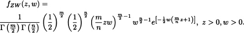
Therefore, the joint probability density function of ![]() and W := Y is given by
and W := Y is given by
![]()
where:
![]()
Integration of fZW(z, w) with respect to w yields the density function of the random variable Z which is then given by:
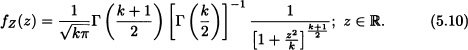
A real-valued random variable Z is said to have a t-Student distribution with k degrees of freedom, notated as ![]() , if its density function is given by (5.10).
, if its density function is given by (5.10). ![]()
Let X and Y be independent random variables such that ![]() and
and ![]() . Consider the map
. Consider the map
![]()
The inverse of g is given by
![]()
and has a Jacobian equal to ![]() . Therefore, the joint probability density function of
. Therefore, the joint probability density function of ![]() and W := Y is given by:
and W := Y is given by:
Integrating with respect to w we find that the density function of Z is given by the following expression:
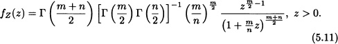
A random variable Z is said to have an F distribution, with m degrees of freedom on the numerator and n degrees of freedom in the denominator, notated as ![]() , if its density function is given by (5.11).
, if its density function is given by (5.11). ![]()
The transformation theorem can be generalized in the following way:
Theorem 5.12 Let X = (X1, X2, · · ·, Xn) be a random vector with joint probability density function fX. Let g be a map of ![]() into itself. Suppose that
into itself. Suppose that ![]() can be partitioned in k disjoint sets A1, · · ·, Ak in such a way that the map g restricted to Ai for i = 1, · · ·, k is a one-to-one map with inverse hi. If the partial derivatives of hi exist and are continuous and if the Jacobians Ji are not zero on the range of the transformation for i = 1, · · ·, k, then the random vector Y := g(X) has joint probability density function given by:
can be partitioned in k disjoint sets A1, · · ·, Ak in such a way that the map g restricted to Ai for i = 1, · · ·, k is a one-to-one map with inverse hi. If the partial derivatives of hi exist and are continuous and if the Jacobians Ji are not zero on the range of the transformation for i = 1, · · ·, k, then the random vector Y := g(X) has joint probability density function given by:
![]()
Proof: Interested reader may refer to Jacod and Protter (2004) for the above theorem. ![]()
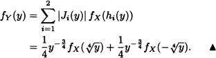
Let X be a random variable with density function fX. Let ![]() be given by g(x) = x4. Clearly
be given by g(x) = x4. Clearly ![]() = (–∞, 0) ∪ [0, ∞) and the maps
= (–∞, 0) ∪ [0, ∞) and the maps
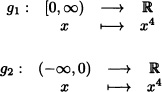
have respectively the inverses
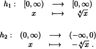
The Jacobians of the inverse transforms are given, respectively, by:
![]()
Therefore, the density function of the random variable Y = X4 is given by:
5.4 COVARIANCE AND CORRELATION COEFFICIENT
Next, the expected value of a function of an n-dimensional random variable is defined.
Definition 5.8 (Expected Value of a Function of a Random Vector)
Let (X1,X2, ...,Xn) be an n-dimensional random vector and let g(.,...,.) be a real-valued function defined over ![]() . The expected value of the function g(X1, ..., Xn), notated as E(g(X1, ..., Xn)), is defined as
. The expected value of the function g(X1, ..., Xn), notated as E(g(X1, ..., Xn)), is defined as
E(g(X1,…,Xn)) :=
provided that the multiple summation in the discrete case or the multiple integral in the continuous case converges absolutely.
Suppose that a fair dice is rolled twice in a row. Let X :=“the maximum value obtained” and Y :=“the sum of the results obtained”. In this case, ![]() .
. ![]()
Let (X, Y, Z) be a three-dimensional random vector with joint probability density function given by:
![]()
Then ![]() and
and ![]() .
. ![]()
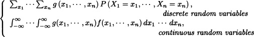
Theorem 5.13 If X and Y are random variables whose expected values exist, then the expected value of X + Y also exists and equals the sum of the expected values of X and Y.
Proof: We prove the theorem for the continuous case. The discrete case can be treated analogously.
Suppose that f is the joint probability density function of X and Y. Then:
![]()
Therefore, E(X + Y) exists.
Furthermore:
Note 5.11 If X is a discrete random variable and Y is a continuous random variable, the previous result still holds.
In general we have the following:
Theorem 5.14 If X1, X2, ..., Xn are n random variables whose expected values exist, then the expected value of the sum of the random variables exists as well and equals the sum of the expected values.
Proof: Left as an exercise for the reader. ![]()
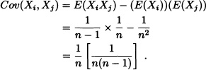
An urn contains N balls, R of which are red-colored while the remaining N – R are white-colored. A sample of size n is extracted without replacement. Let X be the number of red-colored balls in the sample. Prom the theory described in Section 3.2, it is known that X has a hypergeometric distribution of parameters n, R and N; therefore ![]() . We are now going to deduce the same result by writing X as the sum of random variables and then applying the last theorem.
. We are now going to deduce the same result by writing X as the sum of random variables and then applying the last theorem.
Let Xi, with i = 1, ..., n, be the random variables defined as follows:
![]()
![]()
Accordingly:
![]()
Theorem 5.15 If X and Y are independent random variables whose expected values exist, then the expected value of XY also exists and equals the product of the expected values.
Proof: We prove the theorem for the continuous case. The discrete case can be treated analogously.
Suppose that f is the joint probability density function of X and Y. Then:
That is, E(XY) exists.
Suppressing the absolute-value bars on the previous proof, we obtain:
E(XY) = E(X)E(Y).
![]()
Two random variables can be independent or be closely related to each other. It is possible, for example, that the random variable Y will increase as a result of an increment of the random variable X or that Y will increase as X decreases. The following quantities, known as the covariance and the correlation coefficient, allow us to determine if there is a linear relationship of this type between the random variables under consideration.
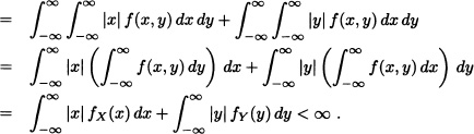
Definition 5.9 (Covariance) Let X and Y be random variables defined over the same probability space and such that E(X2) < ∞ and E(Y2) < ∞. The covariance between X and Y is defined by:
Cov(X, Y) := E((X – E(X))(Y – E(Y))).
Note 5.12 Let X and Y be random variables defined over the same probability space and such that E(X2) < ∞ and E(Y2) < ∞. Since |X| ≤ 1+X2, then it follows that E(X) exists. On the other hand, |XY| ≤ X2 + Y2 implies the existence of the expected value of the random variable (X – E(Y))(Y – E(Y)).
Theorem 5.16 Let X and Y be random variables defined over the same probability space and such that E(X2) < ∞ and E(Y2) < ∞. Then:
(i) Cov(X,Y) = E(XY) – E(X)E(Y).
(ii) Cov(X,Y) = Cov(Y,X).
(iii) Var X = Cov(X,X).
(iv) Cov(aX + b,Y) = a Cov(X,Y) for any a,b ![]()
![]() .
.
Proof: We prove (iv) and leave the others as exercises for the reader:
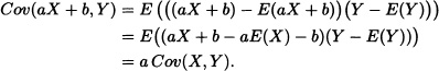
![]()
Note 5.13 From the first property above, it follows that if X and Y are independent, then Cov(X,Y) = 0. The converse, however, does not always hold, as the next example illustrates.
Let Ω = {1,2,3,4}, ![]() = ℘(Ω) and let P :
= ℘(Ω) and let P : ![]() → [0,1] be given by
→ [0,1] be given by ![]() ,
, ![]() . The random variables X and Y defined by X(1) = Y(2) := 1, X(2) = Y(1) := –1, X(3) = Y(3) := 2 and X(4) = Y(4) := –2 are not independent in spite of the fact that Cov(X,Y) = 0.
. The random variables X and Y defined by X(1) = Y(2) := 1, X(2) = Y(1) := –1, X(3) = Y(3) := 2 and X(4) = Y(4) := –2 are not independent in spite of the fact that Cov(X,Y) = 0. ![]()
Theorem 5.17 (Cauchy-Schwarz Inequality) Let X and Y be random variables such that E(X2) < ∞ and E(Y2) < ∞. Then |E(XY)|2 ≤ (E(X2))(E(Y2)). Furthermore, the equality holds if and only if there are real constants a and b, not both simultaneously zero, such that P(aX + bY = 0) = 1.
Proof: Let α = E(Y2) and β = –E(XY). Clearly α ≥ 0. Since the result is trivially true when α = 0, let us consider the case when α > 0. We have:
0 ≤ E((αX + βY)2) = E(α2X2 + 2αβXY + β2Y2)
= α(E(X2)E(Y2) – E(XY)E(XY)).
Since α > 0, the result follows.
If (EXY)2 = E(X2)E(Y2), then E(αX + βY)2 = 0. Therefore, with probability 1, we have that (αX + βY) = 0. If α > 0, we can take a = α and b = β. If α = 0, then we can take a = 0 and b = 1.
Conversely, if there are real numbers a and b not both of them zero such that with probability 1 (aX + bY) = 0, then, aX = –bY with probability 1, and in that case it can be easily verified that |E(XY)|2 = E(X2)E(Y2). ![]()
Note 5.14 Taking |X| and |Y| instead of X and Y in the previous theorem yields:
![]()
Applying this last result to the random variables X – E(X) and Y – E(Y) we obtain ![]() .
.
Theorem 5.18 If X and Y are real-valued random variables having finite variances, then Var(X + Y) < ∞ and we have:
Proof: To see that Var(X + Y) < ∞ it suffices to verify that:
E(X + Y)2 < ∞.
To this effect:
E(X + Y)2 = E(X2) + 2 E(XY) + E(Y2)
≤ E(X2) + 2E|XY| + E(Y2)
≤ 2(E(X2) + E(Y2)) < ∞.
Applying the properties of the expected value, we arrive at (5.12). ![]()
In general we have:
Theorem 5.19 If X1, X2, ..., Xn are n random variables having finite variances, then ![]() and:
and:
![]()
Proof: Left as an exercise for the reader.![]()
Note 5.15 Since each pair of indices i,j with i ≠ j appears twice in the previous summation, it is equivalent to:
![]()
If X1, X2, ..., Xn are n independent random variables with finite variances, then:
![]()
A person is shown n pictures of babies, all corresponding to well-known celebrities, and then asked to whom they belong. Let X be the random variable representing the number of correct answers. Find E(X) and Var(X).
Solution: Let:
![]()
Then:
![]()
Hence:
![]()
On the other hand, we have that:
![]()
Noting that
![]()
and
it follows that
![]()
The covariance is a measure of the linear association between two random variables. A “high” covariance means that with probability 1 there is a linear relationship between the two variables. But what exactly does it mean that the covariance is “high”? How can we qualify the magnitude of the covariance? In fact, property (iv) of the covariance shows that its magnitude depends on the measure scale used. For this reason, it is difficult in concrete cases to determine by inspection if the covariance between two random variables is “high” or not. In order to get rid of this complication, the English mathematician Karl Pearson, who developed most of the modern statistical techniques, introduced the following concept:
Definition 5.10 (Correlation Coefficient) Let X and Y be real-valued random variables with 0 < Var(X) < ∞ and 0 < Var(Y) < ∞. The correlation coefficient between X and Y is defined as follows:
![]()
Theorem 5.20 Let X and Y be real-valued random variables with 0 < Var(X) < ∞ and 0 < Var(Y) < ∞.
(i) ρ(X,Y) = ρ(Y, X).
(ii) |ρ(X,Y)| ≤ 1.
(iii) ρ(X,X) = 1 and ρ(X, –X) = –1.
(iv) ρ(aX + b,Y) = ρ(X, Y) for any a, b ![]()
![]() with a > 0.
with a > 0.
(v) |ρ(X;Y)| = 1 if and only if there are constants a, b ![]()
![]() not both of them zero and c
not both of them zero and c ![]()
![]() such that P(aX + bY = c) = 1.
such that P(aX + bY = c) = 1.
Proof: We prove (ii) and (v) and leave the others as exercise for the reader.
(ii) Let:
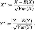
Clearly E(X*) = E(Y*) = 0 and Var(X*) = Var(Y*) = 1. Therefore
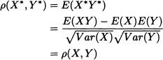
and
0 ≤ Var(X*±Y*) = Var(X*)±2Cov(X*,Y*)+Var(Y*) = 2(1±ρ(X,Y)).
Hence, it follows that:
|ρ(X,Y)| ≤ 1.
(v) Let X* and Y* be defined as in (ii). Clearly
where:
![]()
The case ρ(X,Y) = –1 can be handled analogously.
Part (v) above indicates that if ρ(X,Y)| ≈ 1, then Y(![]() ) ≈ aX(
) ≈ aX(![]() ) + b for all
) + b for all ![]()
![]() Ω. In practice, a “high” absolute-value correlation coefficient indicates that Y can be predicted from X and vice versa.
Ω. In practice, a “high” absolute-value correlation coefficient indicates that Y can be predicted from X and vice versa.
![]()
5.5 EXPECTED VALUE OF A RANDOM VECTOR AND VARIANCE-COVARIANCE MATRIX
In this section we generalize the concepts of expected value and variance of a random variable to a random vector.
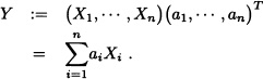
Definition 5.11 (Expected Value of a Random Vector) Let X = (X1, X2, ...,Xn) be a random vector. The expected value (or expectation) of X, notated as E(X), is defined as
E(X) := (E(X1),E(X2),... , E(Xn))
subject to the existence of E(Xj) for all j = 1, ..., n.
This definition can be extended even further as follows:
Definition 5.12 (Expected Value of a Function of a Random Vector) Let X = (X1, X2, ..., Xn) be a random vector and let ![]() be the function given by
be the function given by
h(x1, ..., xn) = (h1(x1, ..., xn), ..., hm(x1, ..., xn))
where hi, for i = 1, ..., m, are real-valued functions defined over ![]() . The expected value of h(X) is given by
. The expected value of h(X) is given by
![]()
subject to the existence of E(hj(X)) for all j = 1, ..., m.
Definition 5.13 (Expected Value of a Random Matrix) If Xij, with i = 1, ..., m and j = 1,..., n, are real-valued random variables defined over the same probability space, then the matrix A = (Xij)m×n is called a random matrix, and its expected value is defined as the matrix whose entries correspond to the expectations of the random variables Xij, that is
E(A) := (E(Xij))m×n
subject to the existence of E(Xij) for all i = 1, ..., m and all j = 1, ..., n.
Definition 5.14 (Variance-Covariance Matrix) Let X = (X1, X2,..., Xn) be a random vector such that ![]() for all j = 1, ..., n. The variance-covariance matrix, notated
for all j = 1, ..., n. The variance-covariance matrix, notated ![]() , of X is defined as follows:
, of X is defined as follows:
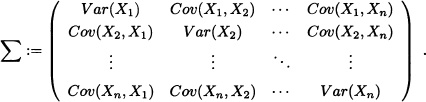
Note 5.16 Observe that ![]() = E([X – E(X)]T [X – E(X)]).
= E([X – E(X)]T [X – E(X)]).
Let X1 and X2 be discrete random variables having the joint distribution given by:
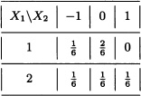
Clearly, the expected value of X = (X1, X2) equals
![]()
and the variance-covariance matrix is given by:
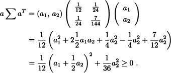
For any a = (a1, a2) we see that:
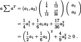
That is, the matrix ![]() positive semidefinite.
positive semidefinite. ![]()
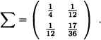
Let X = (X, Y) be a random vector having the joint probability density function given by:
![]()
In this case we have:
Therefore, the expected value of X is given by
![]()
and its variance-covariance matrix equals:
And for any ![]() we have:
we have:
That is, the matrix ![]() is positive semidefinite.
is positive semidefinite. ![]()
In general, we have the following result:
Theorem 5.21 Let X = (X1,..., Xn) be an n-dimensional random vector. If ![]() for all j = 1, ..., n, then the variance-covariance matrix Σ of X is positive semidefinite.
for all j = 1, ..., n, then the variance-covariance matrix Σ of X is positive semidefinite.
Proof: Let a = (a1,..., an) be any vector in ![]() . Consider the random variable Y defined as follows:
. Consider the random variable Y defined as follows:
Since Var(Y) ≥ 0, it suffices to verify that Var(Y) = a Σ aT.
Indeed:
Var(Y) = E([Y – E(Y)]2).
Seeing that, ![]() , where μ := E(X), we have:
, where μ := E(X), we have:
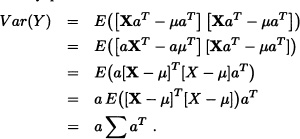
![]()
Note 5.17 Clearly, from the definition of the variance-covariance matrix Σ, if the random variables X1, X2 ..., Xn are independent, then Σ is a matrix whose diagonal elements correspond to the variances of the random variables Xj for j = 1,..., n.
We end this section by introducing the correlation matrix, which plays an important role in the development of the theory of multivariate statistics.
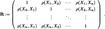
Definition 5.15 (Correlation Matrix) Let X = (X1, X2, ..., Xn) be a random vector with 0 < Var(Xj) < ∞ for all j = 1,..., n. The correlation matrix of X, notated as R, is defined as follows:
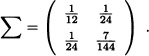
Let X = (X, Y) be a two-dimensional random vector with joint probability density function given by:
![]()
We have
and
Therefore the correlation matrix is given by:
![]()
Note 5.18 The correlation matrix R inherits all the properties of the variance-covariance matrix Σ because
![]()
where ![]() for j = 1, ..., n.
for j = 1, ..., n.
Therefore, R is symmetric and positive semidefinite. Furthermore, if σj > 0 for all j = 1, ..., n, then R is nonsingular if and only if Σ is nonsingular.
5.6 JOINT PROBABILITY GENERATING, MOMENT GENERATING AND CHARACTERISTIC FUNCTIONS
This section is devoted to the generalization of the concepts of probability generating, moment generating and characteristic functions, introduced in Chapter 2 for the one-dimensional case, to n-dimensional random vectors.
Now, we define the joint probability generating function for n-dimensional random vectors.
Definition 5.16 Let X = (X1, X2, ..., Xn) be an n-dimensional random vector with joint probability mass function PX1, X2, ..., Xn). Then the pgf of a random vector is defined as
![]()
for |s1| ≤ 1, |s2| ≤ 1, ..., |sn| ≤ 1 provided that the series is convergent.
Theorem 5.22 The pgf of the marginal distribution of Xi is given by
GXi = GX(1,1, ..., Si, ...,1)
and the pgf of X1 + X2 +...+ Xn is given by
H(s) = GX(s,s, ..., s).
Proof: Left as an exercise. ![]()
Now, we present the pgf for the sum of independent random variables.
Theorem 5.23 Let X and Y be independent nonnegative integer-valued random variables with pgf’s PX(s) and PY(s), respectively, and let Z = X + Y. Then:
GZ(s) = GX + Y(s) = GX(s) · GY(s).
Proof:
![]()
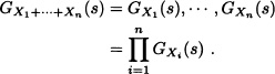
Corollary 5.1 If X1, X2, ..., Xn are independent nonnegative integer-valued random variables with pgf’s GX1(s), ... , GXn(s) respectively, then:
Find the distribution of the sum of n independent random variables Xi, i = 1,2, ..., n, where ![]() Poisson(λ).
Poisson(λ).
Solution: GXi(s) = eλi(s–1). So
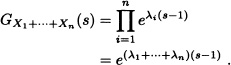
This means that:
If X1, X2, ... , Xn are i.i.d. random variables, then:
GX1+X2+...+Xn(s) = (GXi(s))n.
Theorem 5.24 Let X1, X2, ... be a sequence of i.i.d. random variables with pgf P(s). We consider the sum SN = X1 + X2 + ... + XN where N is a discrete random variable independent of the Xi’s with distribution given by P(N = n) = gn. The pgf of N is ![]() .
.
We prove that the pgf of SN is H(s) = G(P(s)).
Proof:
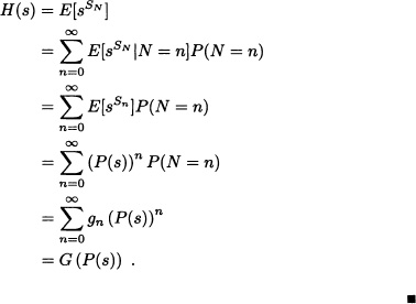
From the above result, we immediately obtain:
1. E(SN) = E(N)E(X).
2. Var(SN) = E(N)Var(X) + Var(N)[E(X)]2.
Now we generalize the concept of mgf for random vectors.
Definition 5.17 (Joint Moment Generating Function) Let X = (X1, ..., Xn) be an n-dimensional random vector. If there exist M > 0 such that ![]() is finite for all t = (t1, ...,tn)
is finite for all t = (t1, ...,tn) ![]()
![]() with
with
![]()
then the joint moment generating function of X, notated as mx(t), is defined as:
![]()
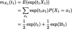
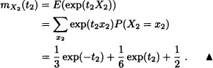
Let X1 and X2 be discrete random variables with joint distribution given by:
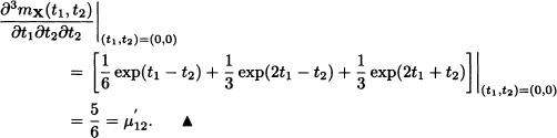
The joint moment generating function of X = (X1, X2) is given by:
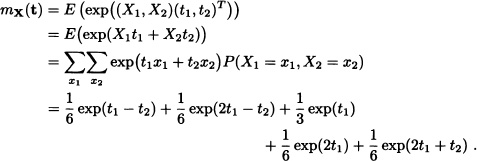
Notice that the moment generating functions of X1 and X2 also exist and are given, respectively, by
and
In general we have the following result:
Theorem 5.25 Let X = (X1, ..., Xn) be an n-dimensional random vector. The joint moment generating function of X exists if and only if the marginal moment generating functions of the random variables Xi for i = 1, ..., n exist.
Proof:
![]() ) Suppose initially that the joint moment generating function of X exists. In that case, there is a constant M > 0 such that mX(t) = E(exp(XtT)) < ∞ for all t with ||t|| < M. Then, for all i = 1, ..., n we have:
) Suppose initially that the joint moment generating function of X exists. In that case, there is a constant M > 0 such that mX(t) = E(exp(XtT)) < ∞ for all t with ||t|| < M. Then, for all i = 1, ..., n we have:
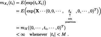
That is, the moment generating function of Xi for i = 1, ... , n exist.
![]() ) Suppose now that the moment generating functions of the random variables Xi for i = 1, ..., n exist. Then, for each i = 1, ..., n there exist Mi > 0 such that
) Suppose now that the moment generating functions of the random variables Xi for i = 1, ..., n exist. Then, for each i = 1, ..., n there exist Mi > 0 such that ![]() < ∞ whenever |ti| < Mi. Let
< ∞ whenever |ti| < Mi. Let ![]() be defined by:
be defined by:
![]()
The function h so defined is convex, and consequently, if xi ![]() , for i = 1, ..., m, and we choose αi
, for i = 1, ..., m, and we choose αi ![]() (0,1) for i = 1, ..., m such that
(0,1) for i = 1, ..., m such that ![]() then, we must have that:
then, we must have that:
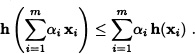
Therefore:
![]()
In particular, for ![]()
n = m, the preceding expression yields:
![]()
Taking expectations we get:
![]()
Therefore, if for a fixed choice of αi ![]() (0,1), i = 1, ..., n, satisfying =
(0,1), i = 1, ..., n, satisfying = ![]() we define
we define ![]() by
by
![]()
E(exp(XuT)) < ∞
and furthermore, by taking M := min{α1M1, ..., αnMn}, for all t ![]()
![]() with ||t|| < M we can guarantee that:
with ||t|| < M we can guarantee that:
E(exp(XtT)) < ∞.
That is, the joint moment generating function of X exists.
The previous theorem establishes that the joint moment generating function of the random variables X1, ..., Xn, exists if and only if the marginal moment generating functions also exist; nevertheless, it does not say that the joint moment generating function can be found from the marginal distributions. That is possible if the random variables are independent, as stated in the following theorem:
Theorem 5.26 Let X = (X1, ...,Xn) be an n-dimensional random vector. Suppose that for all i = 1, ..., n there exists Mi > 0 such that:
![]()
If the random variables X1, ..., Xn are independent, then mx(t) < ∞ for all t = (t1, ..., tn) with ||t|| < M, where M := min{M1, ...,Mn}. Moreover:
![]()
Proof: We have that:
Just like the one-dimensional case, the joint moment generating function allows us, when it exists, to find the joint moment of the random vector X around the origin in the following sense:
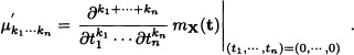
Definition 5.18 (Joint Moment) Let X = (X1, ...,Xn) be an n-dimensional random vector. The joint moment of order k1, ..., kn, with kj ![]()
![]() , of X around the point a = (a1, ..., an) is defined by
, of X around the point a = (a1, ..., an) is defined by
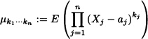
provided that the expected value above does exist.
The joint moment of order k1, ..., kn of X around the origin is written? ![]()
Note 5.19 If X and Y are random variables whose expected values exist, then the joint moment of order 1,1 of the random vector X = (X, Y) around a = (EX,EY) is:
μ11 = E((X – EX)(Y – EY)) = Cov(X, Y).
Let X1 and X2 be the random vectors with joint distribution given by:
We have:
On the other hand:

Furthermore, it can be easily verified that:
The property observed in the last example holds in more general situations, as the following theorem (given without proof) states.
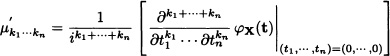
Theorem 5.27 Let X = (X1, ..., Xn) be an n-dimensional random vector. Suppose that the joint moment generating function mx(t) of X exists. Then the joint moments of all orders, around the origin, are finite and satisfy:
We end this section by presenting the definition of the joint characteristic function of a random vector.
Definition 5.19 (Joint Characteristic Function) Let X = (X1, ..., Xn) be an n-dimensional random vector and ![]() . The joint characteristic function of a random vector X, notated as φx(t), is defined by
. The joint characteristic function of a random vector X, notated as φx(t), is defined by
![]()
where ![]() .
.
Just like the univariate case, the joint characteristic function of a random vector always exists. Another property carried over from the one-dimensional case is that the joint characteristic function of a random vector completely characterizes the distribution of the vector. That is two random vectors X and Y will have the same joint distribution function if and only if they have the same joint characteristic function. In addition, it can be proved that successive differentiation of the characteristic function followed by the evaluation at the origin of the derivatives thus obtained yield the presented below expression for the joint moments, around the origin,
whenever the moment is finite.
The proofs of these results given are beyond the scope of this text and the reader may refer to Hernandez (2003).
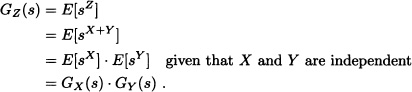
Suppose now that X and Y are independent random variables whose moment generating functions do exist. Let Z := X + Y. Then, we have that:
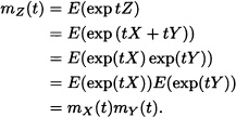
That is, the moment generating function of Z exists and it is equal to the product of the moment generating functions of X and Y.
In general we have that:
Note 5.20 If X1, ..., Xn are n independent random variables whose moment generating functions do exist, then the moment generating function of the random variable Z := X1 +...+ Xn also exists and equals the product of the moment generating functions of X1, ..., Xn. A similar result holds for the characteristic functions and for the probability generating functions.
Let X1, X2, ..., Xn be n independent and identically distributed random variables having an exponential distribution of parameter λ > 0. Then Z := X1 + ...+ Xn has a gamma distribution of parameters n and λ. Indeed, the moment generating function of Z := X1 +...+ Xn is given by
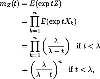
which corresponds to the moment generating function of a gamma distributed random variable of parameters n and λ. ![]()
Suppose you participate in a chess tournament in which you play n games. Since you are an average player, each game is equally likely to be a win, a loss or a tie. You collect 2 points for each win, 1 point for each tie and 0 points for each loss. The outcome of each game is independent of the outcome of every other game. Let Xi be the number of points you earn for game i and let Y equal the total number of points earned over the n games. Find the moment generating function mXi(s) and mY(s). Also, find E(Y) and Var(Y).
Solution: The probability distribution of Xi is:
So the moment generating function of Xi is:
![]()
Since it is identical for all i, we refer to it as mX(s). The mgf of Y is:
![]()
Further:
![]()
![]() EXAMPLE 5.44
EXAMPLE 5.44
Let X1, X2, ...,Xn be n independent and identically distributed random variables having a standard normal distribution and let:
![]()
It is known that if a random variable has a standard normal distribution, then its square has a chi-squared distribution with one degree of freedom. Therefore, the moment generating function of Z is given by

that is, ![]()
![]() EXAMPLE 5.45
EXAMPLE 5.45
Let X1, X2, ... , Xn be n independent random variables. Suppose that ![]() for each k = 1, ...,n. Let α1, ..., αn be n real constants. Then the moment generating function of the random variable Z := α1X1 +...+ αnXn is given by:
for each k = 1, ...,n. Let α1, ..., αn be n real constants. Then the moment generating function of the random variable Z := α1X1 +...+ αnXn is given by:
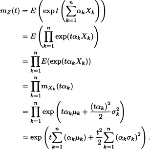
![]()
Let X1, X2, ..., Xn be n independent and identically distributed random variables having a normal distribution of parameters μ and σ2. The random variable ![]() defined by
defined by
![]()
has a normal distribution with parameters μ and ![]() . Consequently:
. Consequently:
EXERCISES
5.1 Determine the constant h for which the following gives a joint probability mass function for (X, Y):
![]()
Also evaluate the following probabilities:
a) P(X ≤ 1,Y ≤ 1) b) P(X + Y ≤ 1) c) P(XY > 0).
5.2 Suppose that in a central electrical system there are 15 devices of which 5 are new, 4 are between 1 and 2 years of use and 6 are in poor condition and should be replaced. Three devices are chosen randomly without replacement. If X represents the number of new devices and Y represents the number of devices with 1 to 2 years of use in the chosen devices, then find the joint probability distribution of X and Y. Also, find the marginal distributions of X and Y.
has the properties 1, 2, 3 and 4 of Theorem 5.3 but it is not a cdf.
5.4 Let (X, Y) a random vector with joint pdf
![]()
5.5 Let X1 and X2 be two continuous random variables with joint probability density function
![]()
Find the joint probability density function of ![]() and Y2 = X1X2.
and Y2 = X1X2.
5.6 (BufFon Needle Problem) Parallel straight lines are drawn on the plane ![]() at a distance d from each other. A needle of length L is dropped at random on the plane. What is the probability that the needle shall meet at least one of the lines?
at a distance d from each other. A needle of length L is dropped at random on the plane. What is the probability that the needle shall meet at least one of the lines?
5.7 Let A, B and C be independent random variables each uniformly distributed on (0,1). What is the probability that Ax2 + Bx + C = 0 has real roots?
5.8 Suppose that a two-dimensional random variable (X, Y) has joint probability density function
a) Find the pdf of ![]() .
.
b) Find E(U).
5.9 Suppose that the joint distribution of the random variables X and Y is given by:
a) P(X ≥ –2, Y ≥ 2).
b) P(X ≥ –2, or Y ≥ 2).
c) The marginal distributions of X and Y.
d) The distribution of Z := X + Y.
5.10 Suppose that two cards are drawn at random from a deck of cards. Let X be the number of aces obtained and Y be the number of queens obtained. Find the joint probability mass function of (X, Y). Also find their joint distribution function.
5.11 Assume that X and Y are random variables with the following joint distribution:
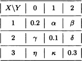
Find the values of α, β, γ, δ, η and κ, so that the conditions below will hold:
P(X = 1) = 0.51, P(X = 2) = 0.22, P(Y = 0) = 0.33 and P(Y = 2) = 0.62.
5.12 An urn contains 11 balls, 4 of them are red-colored, 5 are black-colored and 2 are blue-colored. Two balls are randomly extracted from the urn without replacement. Let X and Y be the random variables representing the number of red-colored and black-colored balls, respectively, in the sample. Find:
a) The joint distribution of X and Y.
b) E(X) and E(Y).
5.13 Solve the previous exercise under the assumption that the extraction takes place with replacement.
5.14 Let X, Y and Z be the random variables with joint distribution given by:
a) E(X + Y + Z).
b) E(XYZ).
5.15 (Multinomial Distribution) Suppose that there are k + 1 different results of a random experiment and that pi is the probability of obtaining the ith result for i = 1, ..., k + 1 (note that ![]() ). Let Xi be the number of times the ith result is obtained after n independent repetitions of the experiment. Verify that the joint density function of the random variables X1, ..., Xk+1 is given by
). Let Xi be the number of times the ith result is obtained after n independent repetitions of the experiment. Verify that the joint density function of the random variables X1, ..., Xk+1 is given by
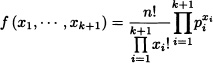
where xi = 0, …, n and ![]()
5.16 Surgeries scheduled in a hospital are classified into 4 categories according to their priority as follows: “urgent”, “top priority”, “low priority” and “on hold”. The hospital board estimates that 10% of the surgeries belong to the first category, 50% to the second one, 30% to the third one and the remaining 10% to the fourth one. Suppose that 30 surgeries are programmed in a month. Find:
a) The probability that 5 of the surgeries are classified in the first category, 15 in the second, 7 in the third and 3 in the fourth.
b) The expected number of surgeries of the third category.
5.17 Let X and Y be independent random variables having the joint distribution given by the following table:
If P(X = 1) = P(X = 2) = ![]() find the values missing from the table. Calculate E(XY).
find the values missing from the table. Calculate E(XY).
5.18 A bakery sells an average of 1.3 doughnuts per hour, 0.6 bagels per hour and 2.8 cupcakes per hour. Assume that the quantities sold of each product are independent and that they follow a Poisson distribution. Find:
a) The distribution of the total number of doughnuts, bagels and cupcakes sold in 2 hours.
b) The probability that at least two of the products are sold in a 15-minutes period.
5.19 Let X and Y be random variables with joint distribution given by:
Find the joint distribution of Z := X + Y and W := X – Y.
5.20 Let X and Y be discrete random variables having the following joint distribution:

Compute Cov(X,Y) and ρ(X,Y).
5.21 Suppose X has a uniform distribution on the interval (–π,π). Define Y = cos X. Show that Cov(X, Y) = 0 though X, Y are dependent.
5.22 An urn contains 3 red-colored and 2 black-colored balls. A sample of size 2 is drawn without replacement. Let X and Y be the numbers of red- colored and black-colored balls, respectively, in the sample. Find ρ(X,Y).
5.23 Let X and Y be independent random variables with ![]() and
and ![]() Calculate P(X = Y).
Calculate P(X = Y).
5.24 Let X1, X2, ...,X5 be i.i.d. random variables with uniform distribution on the interval (0,1).
a) Find the probability that min(X1, X2, ..., X5) lies between ![]() .
.
b) Find the probability that X1 is the minimum and X5 is the maximum among these random variables.
5.25 Let X and Y be independent random variables having Bernoulli distributions with parameter ![]() . Are Z := X + Y and W := X – Y| independent? Explain.
. Are Z := X + Y and W := X – Y| independent? Explain.
5.26 Consider an ”experiment” of placing three balls into three cells. Describe the sample space of the experiment. Define the random variables
N = number of occupied cells
Xi = number of balls in cell number i(i = 1,2,3).
a) Find the joint probability distribution of (N, X1).
b) Find the joint probability distribution of (X1, X2).
c) What is Cov(N, X1)?
d) What is Cov(X1, X2)?
5.27 Let X1, X2 and X3 be independent random variables with finite positive variances ![]() and
and ![]() , respectively. Calculate the correlation coefficient between X1 – X2 and X2 + X3.
, respectively. Calculate the correlation coefficient between X1 – X2 and X2 + X3.
5.28 Let X and Y be two random variables such that ρ(X,Y) = ![]() , Var(X) = 1 and Var(Y) = 2. Compute Var(X – 2Y).
, Var(X) = 1 and Var(Y) = 2. Compute Var(X – 2Y).
5.29 Given the uncorrelated random variable X1, X2, X3 whose means are 2, 1 and 4 and whose variances are 9, 20 and 12:
a) Find the mean and the variance of X1 – 2X2 + 5X3.
b) Find the covariance between X1 + 5X2 and 2X2 – X3 + 5.
5.30 Let X, Y, Z be i.i.d. random variables each having uniform distribution in the interval (1,2). Find Var ![]()
5.31 Let X and Y be independent random variables. Assume that both variables take the values 1 and –1 each with probability ![]() . Let Z := XY. Are X, Y and Z pair-wise independent? Are X, Y and Z independent? Explain.
. Let Z := XY. Are X, Y and Z pair-wise independent? Are X, Y and Z independent? Explain.
5.32 A certain lottery prints n ≥ 2 lottery tickets m of which are sold. Suppose that the tickets are numbered from 1 to n and that they all have the same “chance” of being sold. Calculate the expected value and the variance of the random variable representing the sum of the numbers of the lottery tickets sold.
5.33 What is the expected number of days of the year for which exactly k of r people celebrate their birthday on that day? Suppose that each of the 365 days is just as likely to be the birthday of someone and ignore leap years.
5.34 Under the same assumptions given in problem 5.33, what is the expected number of days of the year for which there is more than one birthday? Verify with a calculator that this expected number is, for all r ≥ 29, greater than 1.
5.35 Let X and Y be random variables with mean 0, variance 1 and correlation coefficient ρ. Prove that:
![]()
Hint: ![]() . Use Cauchy-Schwarz inequality.
. Use Cauchy-Schwarz inequality.
5.36 Let X and Y be random variables with mean 0, variance 1 and correlation coefficient ρ.
a) Show that the random variables Z := X – ρY and Y are not correlated.
b) Compute E(Z) and Var(Z).
5.37 Let X, Y and Z be random variables with mean 0 and variance 1. Let ρ1 := ρ(X,Y), ρ2 := ρ(Y, Z) and ρ3 := ρ(X, Z). Prove that:
![]()
Hint:
XZ = [ρ1Y + (X – ρ1Y)] [ρ2Y + (Z – ρ2Y)].
a) Find ρ(X, Y).
b) Are X and Y independent? Explain.
5.39 Let X and Y be random variables with joint probability density function given by:
![]()
a) Find the value of the constant c.
b) Compute ![]()
c) Calculate E(X) and E(Y).
5.40 Ten costumers, among them John and Amanda, arrive at a store between 8:00 AM and noon. Assuming that the clients arrive independently and that the arrival time of each of them is a random variable with uniform distribution on the interval [0,4]. Find:
a) The probability that John arrives before 11:00 AM.
b) The probability that John and Amanda both arrive before 11:00 AM.
c) The expected number of clients arriving before 11:00 AM.
5.41 Let X and Y be random variables with joint cumulative distribution function given by:
![]()
Does a joint probability density function of X and Y exist? Explain.
5.42 Let X and Y be random variables having the following joint probability density function:
![]()
Compute:
a) The value of the constant c.
b) The marginal density functions of X and Y.
5.43 Let X and Y be random variables with joint probability density function given by:
![]()
Find:
a) ![]() .
.
b) P(Y > 5).
5.44 Andrew and Sandra agreed to meet between 7:00 PM and 8:00 PM in a restaurant. Let X be the random variable representing the arrival time (in minutes) of Andrew and let Y be the random variable representing the arrival time (in minutes) of Sandra. Suppose that X and Y are independent and identically distributed with a uniform distribution over [7,8].
a) Find the joint probability density function of X and Y.
b) Calculate the probability that both Andrew and Sandra arrive at the restaurant between 7:15 PM and 8:15 PM.
c) If the first one waits only 10 minutes before leaving and eating elsewhere, what is the probability that both Sandra and Andrew eat at the restaurant initially chosen?
5.45 The two-dimensional random variable (X, Y) has the following joint probability density function:
![]()
Find:
a) The marginal density functions fX and fY.
b) E(X) and E(Y).
c) Var(X) and Var(Y).
d) Cov(X,Y) and ρ(X,Y).
5.46 Let (X, Y) be the coordinates of a point randomly chosen from the unit disk. That is, X and Y are random variables with joint probability density function given by:
![]()
Compute P(X < Y).
5.47 A point Q with coordinates (X, Y) is randomly chosen from the square [0,1] × [0,1]. Find the probability that (0,0) is closer to Q than ![]()
5.48 Let X and Y be independent random variables with ![]() and
and ![]() . Calculate:
. Calculate:
a) P([X + Y] > 1).
b) P(Y ≤ X2 + 1).
5.49 Let X and Y be independent and identically distributed random variables having a uniform distribution over the interval (0,1). Compute:
a) ![]() .
.
c) ![]()
5.50 Let X and Y be random variables 1having the following joint probability density function:
![]()
Calculate:
a) ![]()
b) ![]()
c) ![]()
5.51 A certain device has two components and if one of them fails the device will stop working. The joint pdf of the lifetime of the two components (measured in hours) is given by:
![]()
Compute the probability that the device fails during the first operation hour.
5.52 Let X and Y be independent random variables. Assume that X has an exponential distribution with parameter λ and that Y has the density function given by ![]() .
.
a) Find a density function for Z := X + Y.
b) Calculate Cov(X, Z).
5.53 Prove or disprove: If X and Y are random variables such that the characteristic function of X + Y equals the product of the characteristic functions of X and F, then X and Y are independent. Justify your answer.
5.54 Let X1 and X2 be two identical random variables which are binomial distributed with parameters n and p. Find the Cov(X1 – X2, X1 + X2).
5.55 Let X and Y be independent and identically distributed random variables having an exponential distribution with parameter λ. Find the density functions of the following random variables:
a) Z:= |X – Y|.
b) W := min{X, Y3}.
5.56 Let X, Y and Z be independent and identically distributed random variables having a uniform distribution over the interval [0,1].
a) Find the joint density function of W := XY and V := Z2.
b) Calculate P(V ≤ W).
5.57 Let X and Y be independent and identically distributed random variables having a standard normal distribution. Let Y1 = X + Y and Y2 = X/Y. Find the joint probability density function of the random variables Y1 and Y2. What kind of distribution does Y2 have?
5.58 Let X and Y be random variables having the following joint probability density function:
![]()
Find the joint probability density function of X2 and Y2.
5.59 Let X and Y be random variables having the joint probability density function given below:
![]()
Calculate the constant c. Find the joint probability density function of X3 and Y3.
5.60 Let X1 < X2 < X3 be ordered observations of a random sample of size 3 from a distribution with pdf
![]()
Show that Y1 = X1/X2,Y2 = X2/X3 and Y3 = X3 are independent.
5.61 Let X, Y and Z be random variables having the following joint probability density function:
![]()
Find fU, where ![]()
5.62 Let X and Y be random variables with joint probability density function given by:
![]()
5.63 Suppose that ![]() Find the value x for which:
Find the value x for which:
a) P(X ≤ x) = 0.99 with m = 7, n = 3.
b) P(X ≤ x) = 0.005 with m = 20, n = 30.
c) P(X ≤ x) = 0.95 with m = 2, n = 9.
5.64 If ![]() , what kind of distribution does X2 have?
, what kind of distribution does X2 have?
5.65 Prove that, if ![]() , then
, then ![]() and
and ![]()
Hint: Suppose that ![]() where U and V are independent,
where U and V are independent, ![]() and
and ![]()
5.66 Let X be a random variable having a t-Student distribution with k degrees of freedom. Compute E(X) and Var(X).
5.67 Let X be a random variable having a standard normal distribution. Are X and |X| independent? Are they not correlated? Explain.
5.68 Let X be an n-dimensional random vector with variance-covariance matrix Σ. Let A be a nonsingular square matrix of order n and let Y := XA.
a) Prove that E(Y) = E(X)A.
b) Compute the variance-covariance matrix of Y.
5.69 If the Yi’s, i = 1, ... ,n, are independent and identically distributed continuous random variables with probability density f(yi), then prove that the joint density of the order statistics Y(1), Y(2), ..., Y(n) is:
![]()
Also, if the Yi, i = 1, ..., n, are uniformly distributed over (0, t), then prove that the joint density of the order statistics is:
![]()
5.70 Let X and Y be independent random variables with moment generating functions given by:
![]()
a) P([X + Y] = 2).
b) E(XY).
5.71 Let, X1, X2, ..., Xn be i.i.d. random variables with a ![]() (μ, σ2) distribution. What kind of distribution do the random variables defined by
(μ, σ2) distribution. What kind of distribution do the random variables defined by ![]() for i = 1,2, ..., n, have? What is the distribution of
for i = 1,2, ..., n, have? What is the distribution of ![]()
5.72 Let X1, X2, ...,Xn be i.i.d. random variables with a ![]() (μ, σ2) distribution. Let
(μ, σ2) distribution. Let
![]()
where:
![]()
What kind of distribution does ![]() have? Explain.
have? Explain.
5.73 The tensile strength for a certain kind of wire has a normal distribution with unknown mean μ and unknown variance σ2. Six wire sections were randomly cut from an industrial roll. Consider the random variables Yi := “tensile strength of the ith segment” for i = 1,2, ...,6. The population mean μ and variance σ2 can be estimated by ![]() and S2, respectively. Find the probability that
and S2, respectively. Find the probability that ![]() is at most at a
is at most at a ![]() distance from the real population mean μ.
distance from the real population mean μ.
5.74 Let X1, X2, ..., Xn be i.i.d. random variables with a ![]() (μ, σ2) distribution. What kind of distribution does the following random variable have:
(μ, σ2) distribution. What kind of distribution does the following random variable have:
Explain.