
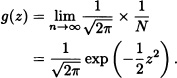
CHAPTER 4
SOME CONTINUOUS DISTRIBUTIONS
In this chapter we will study some of the absolute continuous-type distributions most frequently used.
4.1 UNIFORM DISTRIBUTION
Suppose that a school bus arrives always at a certain bus stop between 6 AM and 6:10 AM and that the probability that the bus arrives in any of the time subintervals, in the interval [0,10], is proportional to the length of the subinterval. This means it is equally probable that the bus arrives between 6:00 AM and 6:02 AM as it is that it arrives between 6:07 AM and 6:09 AM. Let X be the time, measured in minutes, that a student must wait in the bus stop if he or she arrived exactly at 6:00 AM. If throughout several mornings the time of the bus arrival is measured carefully, with the data obtained, it is possible to construct a histogram of relative frequencies. From the previous description it can be noticed that the relative frequencies observed of X between 6:00 and 6:02 AM and between 6:07 and 6:09 AM are practically the same. The variable X is an example of a random variable with uniform distribution. More precisely it can be defined in the following way:
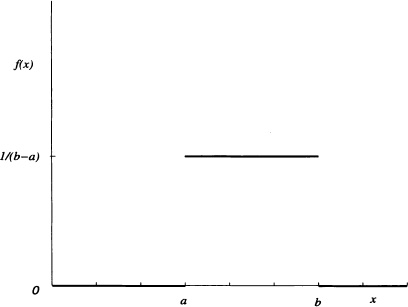
Figure 4.1 Density function of a uniform distribution
Definition 4.1 (Uniform Distribution) It is said that a random variable X is uniformly distributed over the interval [a, b], with a < b real numbers, if its density function is given by:
![]()
The probability density function of a uniform distribution over the interval [a, b] is shown in Figure 4.1.
Notation 4.1 The expression ![]() means that the random variable X has a uniform distribution over the interval [a, b].
means that the random variable X has a uniform distribution over the interval [a, b].
It is easy to verify that if ![]() , then the cumulative distribution function of X is given by:
, then the cumulative distribution function of X is given by:
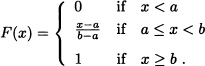
The distribution function of a random variable with uniform distribution over the interval [a, b] is shown in Figure 4.2.
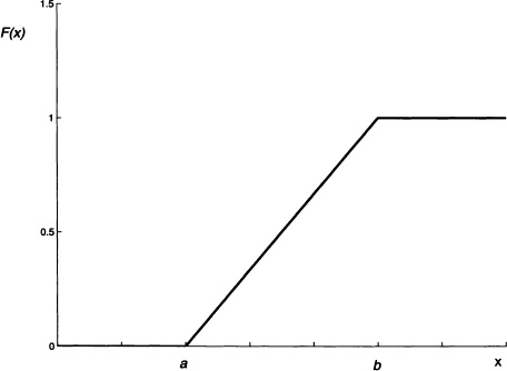
Figure 4.2 Distribution function of a random variable with uniform distribution over the interval [a, b]
Let ![]() . Calculate:
. Calculate:
1. P(X ≥ 0).
2. ![]() .
.
Solution: In this case the density function of the random variable X is given by:
![]()
Therefore,
![]()
and
![]()
Let a, b ![]() be fixed, with a < b. A number X is chosen randomly in the interval [a, b]. This means that any subinterval of [a, b] with length τ has the same probability of containing X. Therefore, for any a ≤ x ≤ y ≤ b, we have that P(x ≤ X ≤ y) depends only on (y − x). If f is the density function of the random variable X, then:
be fixed, with a < b. A number X is chosen randomly in the interval [a, b]. This means that any subinterval of [a, b] with length τ has the same probability of containing X. Therefore, for any a ≤ x ≤ y ≤ b, we have that P(x ≤ X ≤ y) depends only on (y − x). If f is the density function of the random variable X, then:
![]()
This means f(x) = k being k an appropriate constant. Given that
![]()
it can be deduced that ![]() . This is,
. This is, ![]()
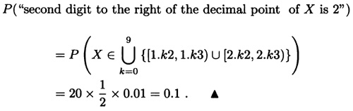
A number is randomly chosen in the interval [1,3]. What is the probability that the first digit to the right side of the decimal point is 5? What is the probability that the second digit to the right of the decimal point is 2?
Solution: Let X := “number randomly chosen in the interval [1,3]”. The density function of the random variable X according to the previous example is:
![]()
Therefore,
and
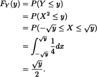
A point X is chosen at random in the interval [−1,3]. Find the pdf of Y = X2.
Solution: For y < 0, FY(y) = 0. For y ![]() [0,1):
[0,1):
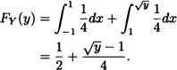
For y ![]() [1,9):
[1,9):
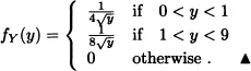
For y ![]() [9, ∞), FY(y) = 1. Hence, the pdf of Y is:
[9, ∞), FY(y) = 1. Hence, the pdf of Y is:
An angle θ is chosen randomly on the interval ![]() . What is the probability distribution of X = tan θ? What would be the distribution of X if θ was to be chosen from (−π/2, π/2)?
. What is the probability distribution of X = tan θ? What would be the distribution of X if θ was to be chosen from (−π/2, π/2)?
Solution: Given that ![]()
![]()
Let X = tan θ. Since tan θ is a strict monotonous and differentiable function in ![]() , by applying Theorem 2.4:
, by applying Theorem 2.4:
![]()
After simplifications, we get:
![]()
When θ is randomly chosen on the interval (−π/2, π/2),
![]()
tan θ is again a strict monotonous and differentiable function. By applying Theorem 2.4, we get:
![]()
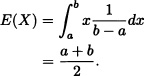
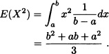
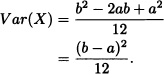
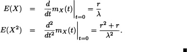
Theorem 4.1 If X is a random variable with uniform distribution over the interval [a, b], then:
1. ![]() .
.
2. ![]() .
.
3. ![]() .
.
Proof:
1.
2.
Therefore:
3. Follows from the definition of the mgf.
![]()
Suppose that ![]() and that E(X) = 2 and
and that E(X) = 2 and ![]() . Calculate P(X ≤ 1).
. Calculate P(X ≤ 1).
Solution: We have that ![]() and
and ![]() . Due to this,
. Due to this, ![]() and
and ![]() . Then:
. Then:
![]()
Note 4.1 Suppose that X is a continuous random variable with increasing distribution function FX(x). Let Y be a random variable with uniform distribution in the interval (0,1) and let Z be a random variable defined as ![]() . The distribution function of the random variable Z is given by:
. The distribution function of the random variable Z is given by:
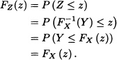
That is, the random variables X and Z have the same probability distribution.
4.2 NORMAL DISTRIBUTION
The normal distribution is one of the most important and mainly used not only in probability theory but also in statistics. Some authors name it Gaussian distribution in honor of Gauss, who is considered the “father” of this distribution. The importance of the normal distribution is due to the famous central limit theorem, which will be discussed in Chapter 8.
Definition 4.2 It is said that a random variable X has normal distribution urith parameters μ, and σ, where μ is a real number and σ is a positive real number, if its density function is given by:
![]()
It is left as an exercise for the reader to verify that f is effectively a density function. That is, f is nonnegative and:
![]()
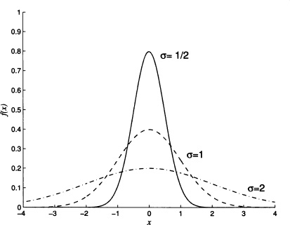
Figure 4.3 Probability density function of normal distribution with μ = 0 and different values of σ
The parameters μ and σ are called location parameter and scale parameter, respectively. We precisely give the concepts to follow.
Definition 4.3 (Location and Scale Parameters) Let Y be a random variable. It is said that θ1 is a location parameter if for all c ![]() we have that a random variable Z := Y + c has parameter θ1 + c. That is, if fY (·; θ1, θ2) is the density function of Y, then the density function of Z is fZ(·; θ1 + c, ·). It is said that θ2 is a scale parameter if θ2 > 0 and for all c
we have that a random variable Z := Y + c has parameter θ1 + c. That is, if fY (·; θ1, θ2) is the density function of Y, then the density function of Z is fZ(·; θ1 + c, ·). It is said that θ2 is a scale parameter if θ2 > 0 and for all c ![]() the random variable W := cY has parameter |c|θ2. That is, if fY(·; θ1, θ2) is the density function of Y, then the density function of W is fW(·; ·, |c|θ2).
the random variable W := cY has parameter |c|θ2. That is, if fY(·; θ1, θ2) is the density function of Y, then the density function of W is fW(·; ·, |c|θ2).
Notation 4.2 We write ![]() to indicate that X is a random variable with normal distribution with parameters μ and σ.
to indicate that X is a random variable with normal distribution with parameters μ and σ.
Figure 4.3 shows the density function of the random variable X with normal distribution with μ = 0 and different values of σ.
In Figure 4.4, it can be seen the density function of the random variable ![]() for σ = 1.41 and different values of μ.
for σ = 1.41 and different values of μ.
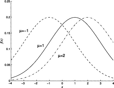
Figure 4.4 Probability density function of normal distribution with σ = 1.41 and different values of μ
The distribution function of the random variable ![]() is given by:
is given by:
![]()
The graph of F, with μ = 0 and σ = 1, is given in Figure 4.5.
Definition 4.4 (Standard Normal Distribution) If ![]() , then it is said that X has a standard normal distribution. The density function and the distribution function of the random variable are denoted by
, then it is said that X has a standard normal distribution. The density function and the distribution function of the random variable are denoted by ![]() and Φ(·), respectively.
and Φ(·), respectively.
Note 4.2 The density function of a standard normal random variable is symmetric with respect to the y axis. Therefore, for all z < 0 it is satisfied that:
![]()
Note 4.3 Let ![]() and let Y := aX + b where a and b are real constants with a ≠ 0. As seen in Chapter 2, it is known that the density
and let Y := aX + b where a and b are real constants with a ≠ 0. As seen in Chapter 2, it is known that the density
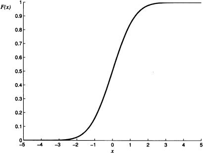
Figure 4.5 Standard normal distribution function with μ = 0 and σ = 1
function of the random variable Y is given by:
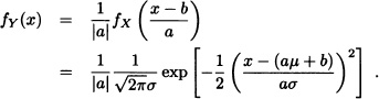
This means Y has a normal distribution with location parameter aμ + b and scale parameter |a|σ. Particularly, if ![]() , then
, then ![]() has a standard normal distribution. That is, in order to know the values of the random variable’s distribution function with arbitrary normal distribution, it is sufficient to know the values of the random variable with standard normal distribution. In Appendix D.3 the table of values of the standard normal distribution are provided.
has a standard normal distribution. That is, in order to know the values of the random variable’s distribution function with arbitrary normal distribution, it is sufficient to know the values of the random variable with standard normal distribution. In Appendix D.3 the table of values of the standard normal distribution are provided.
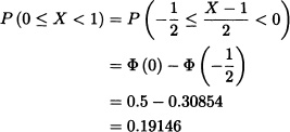
Let ![]() . Calculate:
. Calculate:
1. P(0 ≤ X < 1).
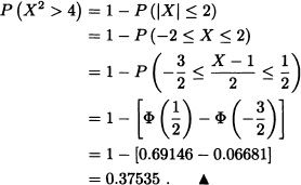
2. P(X2 > 4).
and
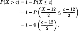
Let ![]() . Find the value of c such that P(X > c) = 0.10.
. Find the value of c such that P(X > c) = 0.10.
Solution:
That is:
![]()
So that the values given in the table we have that:
![]()
and c = 14.57. ![]()
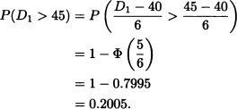
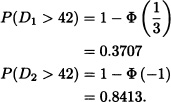
Suppose that the life lengths of two electronic devices say, D1 and D2, have normal distributions ![]() (40,36) and
(40,36) and ![]() (45,9), respectively. If a device is to be used for 45 hours, which device would be preferred? If it is to be used for 42 hours, which one should be preferred?
(45,9), respectively. If a device is to be used for 45 hours, which device would be preferred? If it is to be used for 42 hours, which one should be preferred?
Solution: Given that ![]() and
and ![]() . We will find which device has greater probability of lifetime more than 45 hours:
. We will find which device has greater probability of lifetime more than 45 hours:
Also:
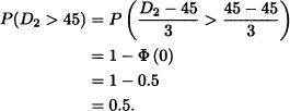
Hence, in this case, the device D2 will be preferred. Now, we will find which device has greater probability of lifetime more than 42 hours. Similar calculation yields:
In this case also, the device D2 will be preferred. ![]()
Let X denote the length of time (in minutes) an automobile battery will continue to crank an engine. Assume that X ~ ![]() (10,4). What is the probability that the battery will crank the engine longer than 10 + x minutes given that it is still cranking at 10 minutes?
(10,4). What is the probability that the battery will crank the engine longer than 10 + x minutes given that it is still cranking at 10 minutes?
![]()
For a specific choice x = 2, we get:
![]()
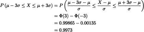
or equivalently P(|X − μ| > 3σ) = 0.0027.
Next, we will find the expected value, the variance and the moment generating function of a random variable with normal distribution.
1. E(X) = μ.
2. Var(X) = σ2.
3. ![]() .
.
Proof: We will calculate the moment generating function. From it, we can easily find the expected value and the variance:
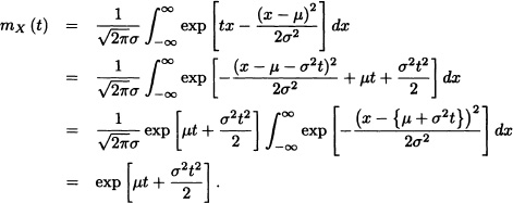
![]()
and
![]()
we get:
![]()
Note 4.5 It can be verified that the characteristic function of the random variable X with normal distribution with parameters μ and σ is given by:
![]()
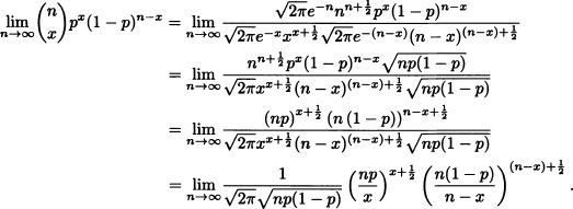
Note 4.6 The normal distribution is another limit form of the binomial distribution only if the following conditions over the parameters n and p are satisfied in the binomial distribution: n → ∞ and if neither p nor q = 1 – p is very small.
Suppose that ![]() . Then:
. Then:
![]()
When n → ∞, we have that x → ∞ and additionally:
![]()
Therefore:
If we take ![]() , we have that Z takes the values
, we have that Z takes the values ![]() . When considering the limit when n → ∞, we have that Z takes all of the values between −∞ and ∞. Isolating x in the previous equation it is obtained that
. When considering the limit when n → ∞, we have that Z takes all of the values between −∞ and ∞. Isolating x in the previous equation it is obtained that ![]() . Replacing in (4.1) we get:
. Replacing in (4.1) we get:
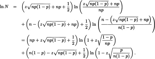
Developing the function h(x) = ln(1 + x), it is obtained:
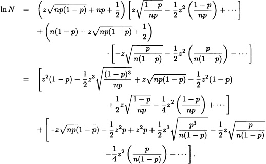
That is:
![]()
![]()
and hence:
![]()
Given that
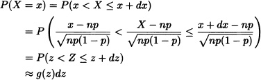
where g(·) is the density function of the random variable Z, and
That is, ![]() . In other words, if n is sufficiently large
. In other words, if n is sufficiently large ![]() . In practice, the approximation is generally acceptable when
. In practice, the approximation is generally acceptable when ![]() and np (1 – p) > 9 or up > 5, or if
and np (1 – p) > 9 or up > 5, or if ![]() and n (1 – p) > 5. In the case of
and n (1 – p) > 5. In the case of ![]() it is obtained that the approximation is quite good even in the case in which n is “small” (see Hernandez, 2003).
it is obtained that the approximation is quite good even in the case in which n is “small” (see Hernandez, 2003).
The result that has recently been deduced is known as the Moivre-Laplace theorem and as it will be seen later on that it is a particular case of the central limit theorem.
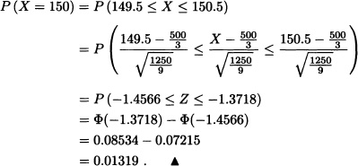
A normal die is tossed 1000 consecutive times. Calculate the probability that the number 6 shows up between 150 and 200 times. What is the probability that the number 6 appears exactly 150 times?
Solution: Let X := “Number of times the number 6 is obtained as a result”. It is clear that ![]() . According to the previous result, it can be supposed that X has a normal distribution with parameters
. According to the previous result, it can be supposed that X has a normal distribution with parameters
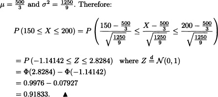
To answer the second part of the question, it may be seen that because the binomial distribution is discrete and the normal distribution is a continuous one, an appropriate approximation is obtained as below:
4.3 FAMILY OF GAMMA DISTRIBUTIONS
Some random variables are always nonnegative and they have distributions that are biased to the right, that is, the greater part of the area below the graph of the density function is close to the origin and the values of the density function decrease gradually when x increases. An example of such distributions is the gamma distribution whose density function is shown in Figure 4.6.
The gamma distribution is used in an extensive way in a variety of areas as, for example, to describe the intervals of time between two consecutive failures of an airplane’s motor or the intervals of time between arrivals of clients to a queue in a supermarket’s cashier point.
The gamma distribution is the generalization of three particular cases that, historically, came first: the exponential function, the Erlang function and the chi-square distribution.
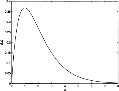
Figure 4.6 Probability density function of a gamma distribution with parameters r = 2 and λ = 1
Definition 4.5 (Gamma Distribution) It is said that the random variable X has gamma distribution with parameters r > 0 and λ > 0 if its density function is given by
where Γ(·) is the gamma function, that is:
![]()
The order of the parameters is important due to the fact that r is the shape parameter while λ is the scale parameter.
The verification that f is a density function is left as an exercise for the reader.
Figure 4.7 shows the gamma density function for λ = 1 and different values of r.
Figure 4.8 shows the form of the gamma density function for r = 1.5 and different values of λ.
Notation 4.3 The expression ![]() means that X has a gamma distribution with parameters r and λ.
means that X has a gamma distribution with parameters r and λ.
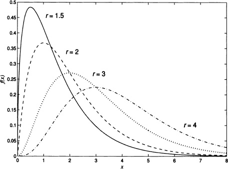
Figure 4.7 Probability density function of a gamma density function for λ = 1 and different values of r
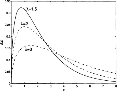
Figure 4.8 Probability density function of a gamma density function for r = 1.5 and different values of λ
The distribution function of the random variable X with gamma distribution with parameters r and λ is given by:
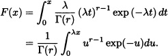
When r is a positive integer, it is known that Γ(r) = (r – 1)! using which we get:
![]()
It can be seen that the right side of the above equation corresponds to P(Y ≥ r) where ![]() . In Chapter 9 we will see that there is a relationship between the Poisson distribution and the gamma distribution.
. In Chapter 9 we will see that there is a relationship between the Poisson distribution and the gamma distribution.
In the following theorem we will determine the expected value, the variance and the moment generating function of a random variable with gamma distribution.
1. ![]() .
.
2. ![]() .
.
3. ![]() if t < λ.
if t < λ.
Proof: We will calculate the moment generating function of X and then, from it, we will find E(X) and Var(X). It is known that:
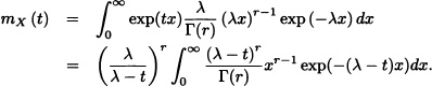
If (λ – t) > 0, then
![]()
is gamma density function, and therefore:
![]()
![]()
Further:
In particular cases, r = 1 and λ > 0, ![]() and
and ![]() with k positive integer, and r > 1 and λ > 0, we get, respectively, the exponential distribution, the chi-square distribution with k degrees of freedom and the Erlang distribution.
with k positive integer, and r > 1 and λ > 0, we get, respectively, the exponential distribution, the chi-square distribution with k degrees of freedom and the Erlang distribution.
Notation 4.4 The expression ![]() indicates that X has an exponential distribution with parameter λ.
indicates that X has an exponential distribution with parameter λ.
The expression ![]() indicates that X has a chi-square distribution with k degrees of freedom.
indicates that X has a chi-square distribution with k degrees of freedom.
The expression ![]() indicates that X has an Erlang distribution with parameters r and λ.
indicates that X has an Erlang distribution with parameters r and λ.
The time (in minutes) required to obtain a response in a human exposed to tear gas A has a gamma distribution with parameter r = 2 and ![]() . The distribution for a second tear gas B is also gamma but has parameters r = 1 and
. The distribution for a second tear gas B is also gamma but has parameters r = 1 and ![]() .
.
1. Calculate the mean time required to get a response in a human exposed to each tear gas formula.
2. Calculate the variance for both distributions.
3. Which tear gas is more likely to cause a human response in less than 1 minute?
Solution: Let X1 X2 be response times from tear gas A and B, respectively.
1. Mean:
![]()
![]()
3. We need to evaluate P(Xi < 1), i = 1, 2.
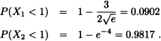
Hence the second tear gas is more likely to cause a human response.![]()
In the next example, we will prove that if ![]() then
then ![]() .
.
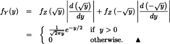
If Z is a standard normal random variable, find the pdf of Y = Z2.
Solution: The cdf of Y is given by:
![]()
Hence,
![]()
where Φ(z) is the cdf of Z. By differentiating the above equation, we obtain:
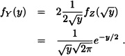
Hence, the pdf of Y is given by:
![]()
Therefore, from equation (4.2) with ![]() and
and ![]() , we conclude that Y has a chi-square distribution with 1 degree of freedom. This problem can also be solved using Corollary 2.2. Since y = z2, then
, we conclude that Y has a chi-square distribution with 1 degree of freedom. This problem can also be solved using Corollary 2.2. Since y = z2, then ![]() .
.
Note 4.7 If ![]() , then
, then ![]() and
and ![]() for t < λ.
for t < λ.
If ![]() , then E(X) = k; Var(X) = 2k and
, then E(X) = k; Var(X) = 2k and ![]() for
for ![]()
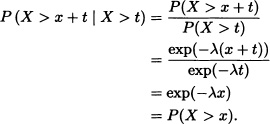
The exponential distribution is frequently used as a model to describe the distribution of the time elapsed between successive occurrences of events, as in the case of the clients who arrive at a bank, calls that enter a call-center, etc. It is also used to model the distribution of the lifetime of components that do not deteriorate or get better through time, that is, those components whose distribution of the remaining lifetime are independent of the actual age. Therefore, this model adjusts to reality only if the distribution of the component’s remaining lifetime does not depend on its age. More precisely, we have the following result:
Theorem 4.4 Let X be a random variable such that P(X > 0) > 0. Then
![]() if and only if P(X > x + t | X > t) = P(X > x)
if and only if P(X > x + t | X > t) = P(X > x)
for all x, t ![]() [0, ∞).
[0, ∞).
Proof: ![]() Suppose that
Suppose that ![]() . Then:
. Then:
![]() Let G(x) = P(X > x). Then, by hypothesis,
Let G(x) = P(X > x). Then, by hypothesis,
![]()
which implies that G(x) = exp(–λx) with λ being a constant greater than 0.
Indeed:
Thus,
![]()
or equivalently:
![]()
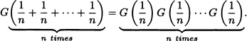
In the same way, we can obtain for m, ![]() the follovring result:
the follovring result:
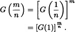
As G is a continuous function to the right, it can be concluded that:
![]()
On the other hand, we have that 0 < G(1) < 1. Indeed, if G(1) = 1, then G(x) = 1, which contradicts that G(∞) = 0. If G(1) = 0 then ![]() and due to the continuity to the right it can be concluded that G(0) = 0, which contradicts the hypothesis. Therefore, we can take λ := – ln [G(1)] in order to obtain the result.
and due to the continuity to the right it can be concluded that G(0) = 0, which contradicts the hypothesis. Therefore, we can take λ := – ln [G(1)] in order to obtain the result. ![]()
The exponential distribution is used in some cases to describe the lifetime of a component. Let T be the random variable that denotes the lifetime of a given component and let f be its density function. It is clear that T is nonnegative. The reliability function of the device is defined by
![]()
where FT(t) is the distribution function of the random variable T. The mean time to failure (MTTF) is defined to be the expected lifetime of the device:
![]()
Suppose that we want to know the probability that the component fails during the next Δt units of time given that it is working correctly until time t. If F is the distribution function of the random variable T and if F(t) < 1, then:
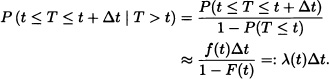
The function λ(t) is known as the risk function or failure rate associated with the random variable T. The function R(t) := 1 – F(t) is also known as the confiability function. The previous expression indicates that if we know the density function of the lifetime of the component, then we know its failure rate. Next, we will see that the converse is also valid. Writing λ(t) as
![]()
and integrating on both sides, we obtain
![]()
That is:
![]()
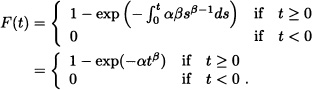
It is reasonable to suppose that F(0) = 0, that is, that the probability of instant failure of the component is zero. In such cases, we have that C = 0 and therefore
![]()
which let us know the distribution function of the random variable T from the risk function. If the failure rate is assumed to be a constant and equal to λ > 0, it can be seen that for t ≥ 0:
![]()
This indicates that the random variable T has an exponential distribution with parameter λ.
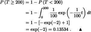
The length of lifetime T, in hours, of a certain device has an exponential distribution with mean 100 hours. Calculate the reliability at time t = 200 hours.
Solution: The density function of the random variable T is given by:
![]()
Therefore:
Let X be the lifetime of an electron tube and suppose that X may be represented as a continuous random variable which is exponentially distributed with parameter λ. Let pj = P(j ≤ X < j + 1). Prove that Pj is of the form (1 – a)aj and determine a.
Solution: For j = 0, 1, ...
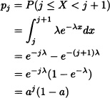
where a = e−λ. Hence we have the result. ![]()
Let X be a uniformly distributed random variable on the interval (0,1). Show that Y = –λ−1ln(1 – X) has an exponential distribution with parameter λ > 0.
Solution: We observe that Y is a nonnegative random variable implying FY(y) = 0 for y < 0. For y > 0, we have:
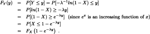
Since ![]() , FX(x) = x, 0 ≤ x ≤ 1. Thus:
, FX(x) = x, 0 ≤ x ≤ 1. Thus:
![]()
so that Y is exponentially distributed with parameter λ. ![]()
4.4 WEIBULL DISTRIBUTION
The Weibull distribution is widely used in engineering as a model to describe the lifetime of a component. This distribution was introduced by a Swedish scientist Weibull who proved that the effort to which the materials are subject to may be modeled through this distribution.
Suppose now that the risk function of a random variable T is given by
![]()
where α and β are positive constants. In such a case we have that:
The density function of T is given by:
![]()
A random variable with the above density function receives a special name:
Definition 4.6 (Weibull Distribution) It is said that a random variable X has Weibull distribution with parameters α and β if its density function is given by:
![]()
Notation 4.5 The expression ![]() indicates that the random variable X has a Weibull distribution with parameters α and β.
indicates that the random variable X has a Weibull distribution with parameters α and β.
Figure 4.9 shows the graph of the Weibull distribution for α = 1 and different values of β.
1. ![]() .
.
2. ![]() .
.
Proof: Left as an exercise. ![]()
Note 4.8 Some authors, for example, Ross (1998) and Hernández (2003), define the density function of a Weibull distribution considering three parameters, a location parameter c, a scale parameter a and a form parameter b, and they say that the random variable X has a Weibull distribution with parameters a, b and c if its density function is given by:
![]()
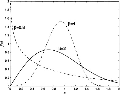
Figure 4.9 Probability density function of a Weibull distribution for α = 1 and different values of β
However, in the majority of the applications it is a common practice to make c = 0, having as a result the density function considered initially by taking ![]() and β = b.
and β = b.
4.5 BETA DISTRIBUTION
The distribution that will be presented here is used frequently as a mathematical model that represents physical variables whose values are restricted to an interval of finite length or as a model for fractions such as purity proportions of a chemical product or the fraction of time that takes to repair a machine.
Definition 4.7 (Beta Distribution) It is said that the random variable X has a beta distribution with parameters a > 0 and b > 0 if its density function is given by
![]()
where B(a, b) is the beta function. That is:
![]()
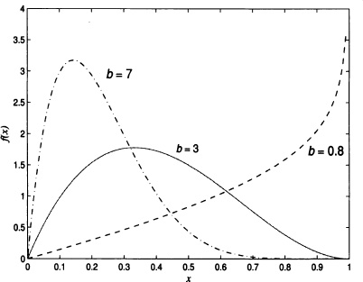
Figure 4.10 Probability density function of a beta distribution for a = 2 and different values of b
Notation 4.6 The expression ![]() means that X has a beta distribution with parameters a and b.
means that X has a beta distribution with parameters a and b.
The beta and gamma functions are related through the following expression:
![]()
so that the density function can be expressed in the form
![]()
If a and b are positive integers, then:
![]()
Figure 4.10 shows the graphs of the beta density function for a = 2 and different values of b.
Figure 4.11 shows the graph of the beta density function with b = 3 and different values of a. It is clear that if a = b = 1, then the beta distribution coincides with the uniform distribution over the interval (0,1). In addition to this, we have that:
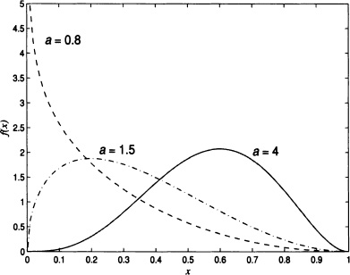
Figure 4.11 Probability density function of beta density function with b = 3 and different values of a
1. If a > 1 and b > 1, the function f has a global maximum.
2. If a > 1 and b < 1, the function f is an increasing function.
3. If a < 1 and b > 1, the function f is a decreasing function.
4. If a < 1 and b < 1, the graph of f has a U form.
The distribution function of the random variable with beta distribution is given by:
![]()
The moment generating function of a random variable with beta distribution does not have a simple form. Due to this, it is convenient to find its moments from the definition.
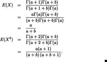
1. ![]() .
.
2. ![]() .
.
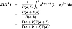
Therefore:
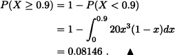
(Wackerly et al., 2008) A gas distributor has storage tanks that hold a fixed quantity of gas and that are refilled every Monday. The proportion of the storage sold during the week is very important for the distributor. Through observations done during several weeks, it was found that an appropriate model to represent the required proportion was a beta distribution with parameters a = 4 and b = 2. Find the probability that the distributor sells at least 90% of his stored gas during a given week.
Solution: Let X := “proportion of the stored gas that is sold during the week”. Given that ![]() we have that:
we have that:
4.6 OTHER CONTINUOUS DISTRIBUTIONS
Definition 4.8 (Cauchy Distribution) It is said that a random variable X has a Cauchy distribution with parameters θ and β, ![]() and
and ![]() , if
, if
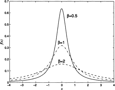
Figure 4.12 Probability density function of a Cauchy distribution for θ = 0 and some values of β
its density function is given by:
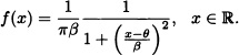
When θ = 0 and β = 1, it is obtained that
![]()
which is known as the standardized Cauchy density function.
Figure 4.12 shows the graphs of f for θ = 0 and some values of β.
Figure 4.13 shows the graphs of f for β = 1 and some values of θ.
The distribution function of the random variable with Cauchy distribution is given by:
![]()
The Cauchy distribution has the characteristic of heavy tails. This means that the values that are farthest away from θ have high probabilities of occurrence. That is why this distribution presents atypical behavior in several ways and is an excellent counterexample for various assertions that in the beginning might seem reasonable. Remember, for example, that in Chapter 2 it was proven that the expected value of the random variable with Cauchy distribution does not exist.
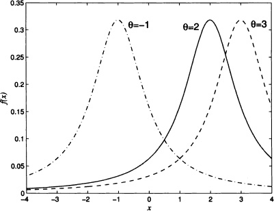
Figure 4.13 Probability density function of a Cauchy distribution for β = 1 and some values of θ
Definition 4.9 (Laplace Distribution) It is said that a random variable X has a Laplace distribution or double exponential with parameters α, β if its density function is given by
![]()
where ![]() and
and ![]() .
.
Figure 4.14 shows the graphs of a Laplace density function with α = 0 and different values of β.
Definition 4.10 (Exponential Power) It is said that a random variable X distributes with an exponential power with parameters α, β and γ with ![]() and β,
and β, ![]() if its density function is given by:
if its density function is given by:
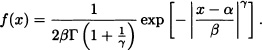
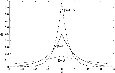
Figure 4.14 Probability density function of a Laplace density function with α = 0 and different values of β
Figure 4.15 Probability density function of an exponential power distribution for a = 0, β = 1 and different values of γ
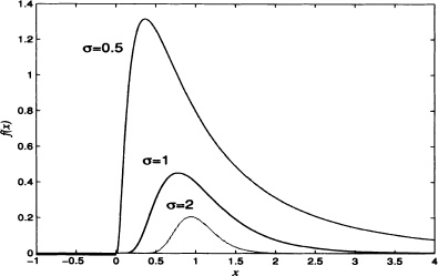
Figure 4.16 Probability density function of a lognormal distribution for μ = 0 and different values of σ
Figure 4.15 shows the graphs of a density function of a random variable with exponential power distribution for α = 0, β = 1 and different values of γ. If γ = 2, then
![]()
that is, we obtain the density function of a random variable with normal distribution with parameters μ = σ and ![]() . If γ = 1 we have that
. If γ = 1 we have that
![]()
which is the Laplace density function with parameters α and β.
Definition 4.11 (Lognormal Distribution) Let X be a nonnegative variable and Y := ln X. If the random variable Y has a normal distribution with parameters μ and σ, then it is said that X has a lognormal distribution with parameters μ and σ.
It is clear that if X has lognormal distribution, its density function is given by:
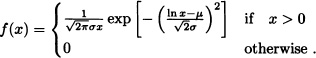
Figure 4.17 Probability density function of a logistic distribution for α = 0 and different values of β
Figure 4.16 shows the graph of a lognormal density function for μ = 0 and different values of σ.
Definition 4.12 (Logistic Distribution) It is said that a random variable X has a logistic distribution with parameters α and β with ![]() and
and ![]() if its density function is given by:
if its density function is given by:
The distribution function of the random variable with logistic distribution of parameters α and β is given by:
![]()
Figure 4.17 shows the graph of the logistic density function for α = 0 and different values of β.
In this chapter we have seen some important distributions of continuous random variables which are frequently used in applications. To conclude this chapter, we now present the relation between various continuous distributions which is illustrated in Figure 4.18.
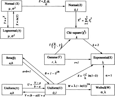
Figure 4.18 Relationship between distributions
EXERCISES
4.1 Let X be a random variable with continuous uniform distribution in the interval ![]() .
.
a) Calculate: mean, variance and standard deviation of X.
b) Determine the value of x so that P(|X| < x) = 0.9.
4.2 A number is randomly chosen in the interval (0,1). Calculate:
a) The probability that the first digit to the right of the decimal point is 6.
b) The probability that the second digit to the right of the decimal point is 1.
c) The probability that the second digit to the right of the decimal point is 8 given that the first digit was 3.
4.3 Let ![]() . If E(X) = 2 and
. If E(X) = 2 and ![]() , which are the values of the parameters a and b?
, which are the values of the parameters a and b?
4.4 A student arrives at the bus station at 6:00 AM sharp knowing that the bus will arrive any moment, uniformly distributed between 6:00 AM and 6:20 AM. What is the probability that the student must wait more than 5 minutes? If at 6:10 AM the bus has not arrived yet, what is the probability that the student has to wait at least 5 more minutes?
4.5 A bus on line A arrives at a bus station every 4 minutes and a bus on line B every 6 minutes. The time interval between an arrival of a bus for line A and a bus for line B is uniformly distributed between 0 and 4 minutes. Find the probability:
a) That the first bus that arrives will be for line A.
b) That a bus will arrive within 2 minutes (for line A or B).
4.6 Assume that N stars are randomly scattered, independently of each other, in a sphere of radius R (measured in parsecs).
a) What is the probability that the star nearest to the center is at a distance at least r?
b) Find the limit of the probability in (a) if R → ∞ and N/R3 → 4πλ/3 where λ ≃ 0.0063.
4.7 Consider a random experiment of choosing a point in an annular disc of inner radius r1 and outer radius r2 (r1 < r2). Let X be the distance of a chosen point from the annular disc to the center of the annular disc. Find the pdf of X.
4.8 Let X be an exponentially distributed random variable with parameter b. Let Y be defined by Y = i for i = 0, 1, 2, ... whenever i ≤ X < i + 1. Find the distribution of Y. Also obtain the variance of Y if it exists.
4.9 Let X be a uniformly distributed random variable on the interval (0,1). Define:
![]()
Find the distribution of Y.
4.10 Suppose that X is a random variable with uniform distribution over the interval (0,4). Calculate the probability that the roots of the equation 2x2 + 2xX + X + 1= 0 are both complex.
4.11 Let X be a random variable with uniform distribution over (−2,2). Find:
a) ![]() .
.
b) A density function of the random variable Y = |X|.
4.12 Let X be a random variable with uniform distribution over (0,1). Find the density functions for the following random variables:
b) Z := X3 + 2.
c) ![]() .
.
4.13 A player throws a dart at a dart board. Suppose that the player receives 10 points for his throw if it hits 2 cm from the center, 5 points if it lands between 2 and 6 cm from the center and 3 points if it hits between 6 and 10 cm from the center. Find the expected number of points obtained by the player knowing that the distance from the place where the dart hits and the center of the board is a random variable with uniform distribution in (0,10).
a) P (−1 < X ≤ 1.2).
b) P (−0.34 < X < 0).
c) P (−2.32 < X < 2.4).
d) P (X ≥ 1.43).
e) P (|X − 1| ≤ 0.5).
4.15 Let ![]() . In each of the following exercises, obtain the value of x that solves the equation:
. In each of the following exercises, obtain the value of x that solves the equation:
a) P(X > x) = 0.5.
b) P(x < X < 5) = 0.1.
c) P(X ≥ x) = 0.01.
4.16 In the following exercises, find the value of c that will satisfy the equalities.
a) P(W ≤ c) = 0.95 if ![]() .
.
b) P(|X – 1| ≤ 3) = c if ![]() .
.
c) P(W > c) = 0.25 if ![]() .
.
d) P(X < c) = 0.990 if ![]() .
.
e) ![]() for k = 3,7,27.
for k = 3,7,27.
4.17 Suppose that the marks on an examination are distributed normally with mean 76 and standard deviation 15. Of the best students 15% obtained A as grade and of the worst students 10% lost the course and obtained P.
a) Find the minimum mark to obtain A as a grade.
b) Find the minimum mark to pass the test.
4.18 The lifetime of a printer is a normal random variable with mean 5.2 years and standard deviation 1.4 years. What percentage of the printers have a lifetime less than 7 years? Less than 3 years? Between 3 and 7 years?
4.19 Let X be a random variable with normal distribution with mean μ and variance σ2. Find the distribution of the random variable Y := 5X – 1.
4.20 Suppose that the lifespan of a certain type of lamp is a random variable having a normal distribution with mean 180 hours and standard deviation 20 hours. A random sample of four lamps is taken.
a) What is the probability that all four lamps have a lifespan greater than 200 hours?
b) All four lamps of the random sample are placed inside an urn. If one lamp is then randomly selected, what is the probability that the extracted lamp has a lifespan greater than 200 hours?
4.21 Let X be a random variable with binomial distribution with parameters n = 30 and p = 0.3. Is it reasonable to approximate this distribution to a normal with parameter μ = 9 and variance σ2 = 6.3? Explain.
4.22 A fair die is tossed 1000 consecutive times. Calculate the probability that the number 3 is obtained less than 500 times given that the number 1 was obtained exactly 200 times.
4.23 Let ![]() . Find the number α so that:
. Find the number α so that:
![]()
4.24 Determine the tenths of the standard normal distribution, that is, the values x0.1, x0.2, ···, x0.9, so that Φ (x0.i) = 0.i for i = 1, ···, 9.
4.25 Consider a nonlinear amplifier whose input X and output Y are related by its transfer characteristic:
![]()
Find the pdf of Y if X has ![]() distribution.
distribution.
4.26 Let X be a continuous random variable with distribution function F and pdf f(x). The truncated distribution of X to the left at X = α and to the right at X = β is defined as:
Find the pdf of a truncated normal ![]() (μ, σ2) random variable truncated to the left at X = α and to the right at X = β.
(μ, σ2) random variable truncated to the left at X = α and to the right at X = β.
4.27 A marketing study determined that the daily demand for a recognized newspaper is a random variable with normal distribution with mean μ = 50,000 and standard deviation σ = 12,500. Each newspaper sold leaves 500 Colombian pesos as revenue, while each paper not sold gives 300 Colombian pesos as loss. How many newspapers are required in order to produce a maximum expected revenue?
4.28 Let X be a random variable with:
a) Uniform distribution over [–1,1].
b) Exponential distribution with parameter λ.
c) Normal distribution with parameters μ and σ.
Calculate the distribution function FY and the density function fY of the random variable Y = aX + b, where a and b are real numbers and a ≠ 0.
4.29 In the claim office of a public service enterprise, it is known that the time (in minutes) that the employee takes to take a claim from a user is a random variable with exponential distribution with mean 15 minutes. If you arrive at 12 sharp to the claim office and in that moment there is no queue but the employee is taking a claim from a client, what is the probability that you must wait for less than 5 minutes to talk to the employee?
4.30 Suppose that the number of kilometers that an automobile travels before its battery runs out is distributed exponentially with a mean value of 10,000 km. If a person wants to travel 5,000km, what is the probability that the person finishes his trip without having to change the battery?
4.31 The time that has elapsed between the calls to an office has an exponential distribution with mean time between calls of 15 minutes.
a) What is the probability that no calls have been received in a 30-minute period of time?
b) What is the probability of receiving at least one call in the interval of 10 minutes?
c) What is the probability of receiving the first call between 5 and 10 minutes after opening the office?
4.32 The length of time T of an electronic component is a random variable with exponential distribution with parameter λ.
a) Determine the probability that the electronic component works for at least until t = 3λ−1.
b) What is the probability that the electronic component works for at least until t = kλ−1 if it work’s until time t = (k – 1)λ−1 ?
4.33 Let X be a random variable having an exponential distribution with parameter ![]() . Compute:
. Compute:
a) P(X > 3).
b) P(X > 6 | X > 3).
c) P(X > t + 3 | X > t).
4.34 Let X be a random variable with exponential distribution with parameter λ. Find the density functions for the following random variables:
a) Y := ln X.
b) Z := X2 + 1.
c) ![]() .
.
a) In 1825 Gompertz proposed the risk function λ(t) given by
![]()
to model the lifetime of human beings. Determine the distribution function F corresponding to the failure function λ(t).
b) In the year 1860 Makeham modified the risk function proposed by Gompertz and suggested the following:
![]()
Determine the distribution function F corresponding to the failure function λ(t) (this distribution is also known as the Makeham distribution).
4.36 Calculate the failure function of the exponential distribution with parameter μ.
4.37 Determine the distribution of F whose failure distribution is given by
![]()
4.38 Suppose that T denotes the lifetime of a certain component and that the risk function associated with T is given by:
![]()
Find the distribution of T.
4.39 Suppose that T denotes the lifetime of a certain component and that the risk function associated with T is given by
![]()
where α > 0 and β > 0 are constants. Find the distribution of T.
4.40 Let X be a Weibull distribution. Prove that Y = bX for some b > 0 has the exponential distribution.
4.41 The lifetime of a certain electronic component has a Weibull distribution with β = 0.5 and a mean life of 600 hours. Calculate the probability that the component lasts at least 500 hours.
4.42 The time elapsed (in months after maintenance) before a fail in a vigilance equipment with closed circuit in a beauty shop has a Weibull distribution with ![]() and β = 2.2. If the shop wants to have a probability of damage before the next programmed maintenance of 0.04, then what is the time elapsed of the equipment to receive maintenance?
and β = 2.2. If the shop wants to have a probability of damage before the next programmed maintenance of 0.04, then what is the time elapsed of the equipment to receive maintenance?
4.43 A certain device has the Weibull failure rate
![]()
a) Find the reliability R(t).
b) Find the mean time to failure.
c) Find the density function fT(t).
4.44 A continuous random variable X is said to have Pareto distribution if it has density function
![]()
The Pareto distribution is commonly used in economics.
a) Find the mean and variance of the distribution.
b) Determine the density function of Z = lnX.
4.45 A certain electrical component of a mobile phone has the Pareto failure rate
![]()
a) Find the reliability R(t) for t > 0.
b) Sketch R(t) for t0 = 1 and a = 2.
c) Find the mean time to failure if a > 0.
4.46 Let X be a random variable with standard normal distribution. Find E(|X|).
4.47 Consider Note 4.1. Let X be a continuous random variable with strictly increasing distribution function F. Let Y = FX (X). Prove that Y has uniform distribution over (0,1).
4.48 Let X be a random variable with uniform distribution over (0,1). Find the function g : ![]() , so that Y = g(X) has a standard normal distribution.
, so that Y = g(X) has a standard normal distribution.
4.49 Prove that if X is a random variable with Erlang distribution with parameters r and λ, then:
![]()
![]()
4.52 Let X be a random variable with standard Cauchy distribution. Prove that E(X) does not exist.
4.53 Let X be a random variable with standard Cauchy distribution. What type of distribution has the random variable ![]() ?
?
4.54 Let X be a normal random variable with parameters 0 and σ2. Find a density function for:
a) Y = |X|.
b) ![]() .
.
4.55 Let X be a continuous random variable with pdf
![]()
![]()
4.56 Let X be a random variable with standard normal distribution. Prove that
![]()