CHAPTER 12

INTRODUCTION TO MATHEMATICAL FINANCE

Mathematical finance is the study of financial markets and is one of the rapidly growing subjects in applied mathematics. This is due to the fact that in recent years mathematical finance has become an indispensable tool for risk managers and investors. The fundamental problem in the mathematics of financial derivatives is the pricing and hedging. During the years 1950–1960, the research focus was basically on the resolution of problems in economics and statistics. However, many researchers were concerned with the problem that was initiated in the early 20th century by Bachelier, the father of modern mathematical finance: what is the fair price for an option on a particular stock? The answer to this question was given in 1973 by researchers Fisher Black and Myron Scholes. They argued that a rational investor does not wait passively until the expiry of the contract but, in contrast, invests in a portfolio consisting of a risk-free asset and a risky stock, so that the value of this portfolio will be equal to the value of the option. Therefore, the fair price of the option is the present value of the portfolio. To obtain this value they generated a partial differential equation whose solution is known as the “Black-Scholes formula”.

The initial focus on the valuations of financial derivatives was to describe the appropriate movements of stock prices and solving partial differential equations. However, another purely probabilistic approach was developed by Cox et al. (1979) among others, who considered the discrete case. Harrison and Kreps (1979) observed that for a market model to be sensible from the economic point of view, the discounted stock price process should be a martingale under an appropriate change of measure. This viewpoint was further expounded by Harrison and Pliska (1981) who observed that by making use of the ltd representation theorem, the present value of the price of an option can be characterized by a stochastic integral and the discounted price of the stock can be transformed into a martingale by a suitable change of measure. This approach is also known as the martingale pricing method or risk-neutral valuation. The objective of this chapter is to introduce risk-neutral valuation within the framework of financial derivatives. We will keep this chapter as simple as possible to present the basic modeling approach for the financial derivatives. In the next section we review the technical terminology used in the financial derivatives. Interested reader may refer to Hull (2009) for more details.

12.1   FINANCIAL DERIVATIVES

Definition 12.1  A financial derivative, or contingent claim, is a financial contract whose value at expiration date T is determined exactly by the price of the underlying financial asset at time T.

The financial derivatives or financial securities are financial contracts whose value is derived from some underlying assets. The assets could be stocks, currencies, equity indices, bonds, interest rates, exchange rates, and commodities. There are different types of financial markets, namely stock markets, bond markets, currency markets, and commodity markets. In general, financial derivatives can be grouped into three groups: options, forwards, and futures. The options constitute an important building block for pricing financial derivatives. Now we give a formal definition for an option.

Definition 12.2  An option is a contract that gives the holder the right but not the obligation to undertake a transaction at a specified price at a future date.

Note 12.1  A specific or prescribed price is called a strike price, denoted by K. A specific or a future time is called an expiry date, denoted by T.

There are two main types of option contracts: call options and put options.

1. A call option gives one the right to buy an asset at a specific price within a specific time period.
2. A put option gives the right to sell an asset at a specific price within a specific time period.

A call option is the right to buy (not an obligation). When a call is exercised, the buyer pays the writer (the other party of the contract, who does have a potential obligation that he must sell the asset if the holder chooses to buy) the strike price and gives up the call in exchange for the asset.

The contract for a call (put) option specifies:

1. The company whose shares are to be bought (sold)
2. The number of shares that can be bought (sold)
3. The purchase (selling) price
4. The date when the right to buy (sell) expires

Based on how they are exercised, options can be divided into two types:

1. European option that can be exercised only at the time of expiry of the contract.
2. An American option that can be exercised at any time up to the expiry date.

The call or put option described above is also called a simple or vanilla option. An option which is not a vanilla option is called an exotic option. The well-known exotic option is a path-dependent option where the payoff depends on the past and present values of an underlying asset. The following exotic options are widely used.

1. An Asian option is a type of option whose payoff function is determined by the average price of an underlying asset over some period of time before expiry.
2. A barrier option is a type of option whose payoff depends on whether or not the underlying asset has reached or exceeded a predetermined price
3. A lookback option is an option whose payoff is determined by the maximum or minimum of the underlying asset.
4. A perpetual option has no expiry date (that is, it has an infinite time horizon).

In the following sections some financial terms are used. The practical meaning of these terms are as follows:

1. Intrinsic value: At time t ≤ T, the intrinsic value of a call option with strike price K is equal to max(S_t − K, 0). Similarly for a put option, the intrinsic value is max(K − S_t, 0).
2. Time value: The time value of an option is the difference between the price of the option and its intrinsic value. That is, for a European call option, the time value is C(S_t, t) = max(S_t − K, 0).
3. Long position: A party assumes a long position by agreeing to buy an asset for the strike price K at expiry date T because he anticipates the price to go up. That is, one can have positive amounts of an asset by buying assets that one does own.
4. Short position: The opposite of assuming a long position in which one party agrees to sell the asset because he anticipates the price to decline. That is, one can have negative amounts of an asset by selling assets that one does not own.
5. Arbitrage: This refers to buying an asset at one place and selling it for a profit at another place without taking any risk. We will give a precise mathematical definition in the next section.
6. Hedging: This is the concept of elimination of risk by taking opposite positions in two assets whose prices are correlated.

Forwards and Futures

Forwards and futures are both contracts to deliver a specific asset at an agreed date in the future at a fixed price. Unlike an option, there is no choice involved as to whether the contract is completed.

Definition 12.3  A forward contract is an agreement to buy or sell an asset S at certain future date T for a certain price K.

A forward contract is usually between large and sophisticated financial agents (banks, institutional investors, large corporations and brokerage firms) and is not traded in an exchange. The agent who agrees to buy the underlying asset is said to have a long position while the other agent assumes a short position. The settlement date is called delivery date and the specified price is referred to as the delivery price.

Two persons or parties can enter into a forward contract to buy or sell Colombian coffee at any time with any delivery date and delivery price they choose. When a forward contract is created at time 0 with delivery date T for delivery price K, this delivery price is also referred as the forward price at time 0 for delivery date T. At the time t between 0 and T, it would be possible to create a new forward contract with the same delivery date T. The delivery price of this new contract is also called the forward price at the time t with delivery date T and might not be the same as the delivery price K which was the delivery price with delivery date T on the contract that was set up at time t = 0.

The disadvantage of forwards is that they are hardly traded at exchanges, the reason being the individual, nonstandardized character of the contract, and that they are exposed to the risk of default by their counter parties. Therefore, there are significant costs in finding a partner for the contract. These problems lead to standardization with the aim of making trading at an exchange possible.

A futures contract, although like a forward contract, differs from it as shown below.

1. A forward is an over-the-counter agreement between two individuals. In contrast, a future is a trade organized by an exchange.
2. A forward is settled on the delivery date. That is, there is a single payment made when the contract is delivered. The profit/loss on a future is settled on a daily basis to avoid default. The exchange acts as an intermediary between the long and short parties and insists on maintained margins.

A basket of forwards and/or options with different delivery or expiry dates is called a swap, which is a more complex financial derivative. A swap is an agreement where two parties undertake to exchange, at known dates in the future, various financial assets (or cash flows) according to a prearranged formula that depends on the value of one or more underlying assets. The two commonly used swaps are interest rate swaps and currency swaps.

The focus of this chapter will be on the pricing and hedging of options. We will restrict ourselves to European and American call and put options. The option buyer has the right but not the obligation, which puts him in a privileged position. The option seller, that is, the option writer, provides the privilege which the buyer holds. We have seen two types of options, namely, option to buy, a call option, and option to sell, a put option. Using asymmetry in rights, there are four possibilities:

1. Buy an option to buy, i.e., buy call
2. Buy an option to sell, i.e., buy put
3. Sell an option to buy, i.e., write call
4. Sell an option to sell, i.e., write put

The payoff, or the value, of an option depends on the value of an underlying asset at a future time T. Consider a European call option with strike price K. Let S_T be the price of the underlying asset at the time of expiry T. If S_T < K, that is the option is expiring out-of-money, then the holder can buy the asset in the market at S_T, a, cost less than the strike price K. The terminal payoff of the long position in a European call option is 0. But if, at time T, S_T > K, that is the option expires in-the-money, then the holder of the call option will choose to exercise the option. The holder can buy the asset at a price K and sell it at a higher price S_T. The net profit will be S_T — K. Both cases can be summarized mathematically as:

Figure 12.1    Payoff diagram of call and put options

C(S_t, T) = max(S_T − K, 0) or C(S_t, T) = (S_T − K)⁺,

where (x)⁺ = max(x, 0). An argument similar to the value of a call option leads to the payoff for a put option at expiry date T and is given by:

P(S_t, T) = max(K − S_T, 0) or P(S_t, T) = (K − S_T)⁺.

A chart of the profits and losses for a particular option is called a payoff diagram and is a plot of the expected profit or loss against the price of the underlying asset on the same future date. The payoff diagrams for call and put options are given in Figure 12.1.

For European options, there is a simple theoretical relationship between the prices of the corresponding call and put options. This important relationship is known as put-call parity and may be expressed as:

C(S_t, T) − S_t = P(S_t, T) − Ke ^−r(T−t),

where K is the strike price of the underlying stock S, T is the expiry date and r is the constant interest rate; sometimes we use C = C(S_t, T) and P = P(S_t, T)

  EXAMPLE 12.1

Suppose that a share of a certain stock is worth $100 today for a strike price of $110 with one year expiry date. The difference between the costs of put and call options is $5. The interest rate is calculated by using put-call parity. We have:

The main assumptions of the options are:

1. There are some market participants.
2. There are no transaction costs.
3. All trading profits (net of trading losses) are subject to the same tax rate.
4. Borrowing and lending at the risk-free rate are possible.

We now establish an interesting result between European and American call options.

Theorem 12.1  With a nonnegative interest rate r, it is not optimal to exercise early an American call option on a non-dividend paying asset with the same strike price and expiry date.

Proof: Suppose that it is optimal to exercise the American call option before expiry date.

Let C_A and C_E be the value of the European and American options, respectively. It is easily seen that the payoff value of the European call options:

C_E = S − Ke^−r(T−t).

We know that:

C_A > C_E

This is because an American option has the benefits of having the right of early exercise. Also, we have:

C_A > S − Ke^−r(T−t).

Since r > 0, it follows that C_A > S − K. An American option will always be worth at least its payoff S − K. However, the previous equation shows that C_A > S − K. Thus, we have a contradiction based on the assumption that it is optimal to exercise early. Hence the value of the American option must be equal to the value of the European call option. However, it can be advantageous to exercise an American put option on a non-dividend paying asset.          

In the continuation we present a discrete-time model and a continuous-time model for the valuation of financial derivatives. We closely follow the approach presented by Lamberton and Lapeyre (1996), Bingham and Kiesel (2004), and Williams (2006).

12.2    DISCRETE-TIME MODELS

In this section we give a brief introduction to discrete-time models of a finite market, , that is, models with a finite number of trading dates in which all asset prices take a finite number of values. The finite market model is considered on a finite probability space (Ω, , P), where Ω = {ω₁, ω₂, …, ω_n}, is a σ-algebra consisting of all subsets of Ω and P is a probability measure on (σ, ) such that P({ω}) > 0, ∀ω; ∊ Ω. We assume that there is a finite number of trading dates t = 0,1,2, …, N where N < ∞ at which trades occur. The time N is the terminal date or maturity of the financial contract considered. We now use a finite filtration to model the information flow over time. Further, and .

We assume that the market consists of k + 1 assets whose prices at time n are given by the nonnegative random variables which are measurable with respect to . We assume that there exists one riskfree asset on the money market, known as a bond, R, and k risky assets or stocks on the financial market, S = (S¹, S², … , S^k).

Definition 12.4  A numeraire is a price process {X_n; n = 0, … , N} which is strictly positive for all n = 0, 1, … , N.

For example, suppose that R₀ = 1. If the return of a bond over a period is a constant r, then R_n = (1 + r)ⁿ. The coefficient is interpreted as the discount factor. For i = 1, 2, … , k, we define:

Then is the vector of discounted stock prices at time n. The investors are interested in creating a dynamic portfolio which involves trading strategies and a portfolio process. Hence we now give the definition of the trading strategies and portfolio or wealth processes.

Definition 12.5  A trading strategy in the finite market model is a collection of k + 1 random variables where is a real-valued measurable random variable for i = 0,1, … , k. We interpret as the number of shares of asset i to be held over the time (n − 1, n].

  EXAMPLE 12.2

For a financial market model with a single bond and a single stock, the trading strategy is a collection of pairs of random variables

φ = {(α_n, β_n); n = 0, 1, … , N}.

The random variable α_n represents the number of shares of stock to be held over the time interval (n — 1, n], and the random variable β_n represents the number of units of the bond to be held over the same time interval. Here both α_n and β_n are measurable and hence are called predictable random variables.     

Definition 12.6 (Value of Portfolio or Wealth Process)  The value of the portfolio or wealth process V_n(φ) of a trading strategy φ at time n equals:

The discounted values are given by .

For simplicity we consider the case of two assets in our model, a risk-free money market account, a bond R, and a risky asset, the stock S. We assume that the stock price is adapted to the filtration (_n) for the trading dates n = 0, 1, 2, … , N.

Definition 12.7  A trading strategy is called self-financing if for all n = 1, … , N :

This implies that no funds are withdrawn from or added the strategy.

Theorem 12.2  A trading strategy φ is self-financing if and only if we have for all n = 1, … , N:

Hence the value of a self-financing strategy consists of the initial investment V₀ and the gains (or losses) from the trade stock and money market account

Proof:  From the definition of the value of a portfolio we get that:

Now φ is self-financing if and only if β_n+1R_n + α_n+1S_n = β_nR_n + α_nS_n for all n = 1, … , N. Substituting this into (12.3) gives:

As , the lemma follows by summing over (12.4).     

We give a similar characterization of a self-financing strategy in terms of the discounted value process.

Theorem 12.3  A trading strategy is self-financing if and only if we have for all n = 1, … , N:

Proof: The proof of this theorem is omitted as it is similar to the proof of the previous theorem.     

Definition 12.8  A trading strategy φ = {(φ_n; n = 1, … , N} is called admissible if it is self-financing with V_n(φ) > 0 for n = 1, 2, … , N.

Definition 12.9 (Arbitrage Opportunity)  An arbitrage opportunity in the financial markets is a trading strategy φ such that V₀ (φ) = 0, V_N(φ) ≥ 0 and E (V_N(φ)) > 0.

Definition 12.10  A finite market model is called viable or arbitrage-free, if there are no arbitrage opportunities.

Note 12.2 (European Contingent Claim)  The value of the European contingent claim (ECC) H ≥ 0 with expiry date N is an _N measurable random variable. The random variable H is a known payoff of the claim. For example, a European call option with strike price K and expiry date N is:

H = max(S_N − K, 0).

Definition 12.11 (Attainable or Replicating Strategy)  Given a finite market model , a contingent claim H with maturity N is called attainable if there is an admissible, self-financing strategy φ_n = (α_n, β_n) such that V_N(φ) = H; φ is called a replicating strategy for the derivative.

Definition 12.12  A finite market M is called complete if every contingent claim is attainable or equivalently, if for every _N -measurable random variable H there exists at least one trading strategy φ such that V_N(φ) = H.

The completeness of the finite market model is a highly desirable property. Under market completeness, any European or American contingent claim can be priced by an arbitrage-free and self-financing strategy. If the market is not complete, then it is called an incomplete market model.

In order to characterize arbitrage-free markets, we use the concept of equivalent martingale measures.

Definition 12.13  Let be a finite market model. A probability measure Q on (Ω, ) such that

1. Q is equivalent to P, i.e., for all we have Q(A) = 0 ⇔ P(A) = 0, and
2. the discounted stock price is a martingale under measure Q

is called an equivalent martingale measure or a risk-neutral measure for .

Note 12.3

1. The measure Q is said to be absolutely continuous with respect to P, i.e., for all we have P(A) = 0 ⇒ Q(A) = 0.
2. A martingale under measure Q is referred as a Q-martingale.

Theorem 12.4  Let Q be an equivalent martingale measure for the market . Consider a self-financing, admissible trading strategy φ. Then the discounted process is a Q-martingale.

Proof:  As φ is self-financing, we get from Theorem 12.3:

As φ is admissible, is -measurable and is a Q-martingale:

Theorem 12.5  If an equivalent martingale measure exists for the finite market model , then the model is arbitrage-free.

Proof: Consider a self-financing strategy φ with . We will show that the existence of an equivalent martingale measure Q gives , which implies that the finite market model is arbitrage-free.

If and have the same sign, then it follows that and

We have that the measure Q is equivalent to P, which implies that > 0 and this gives . We know that is a Q-martingale, which shows that , and therefore, we conclude that .          

We now state the first fundamental theorem of asset pricing.

Theorem 12.6  A finite market is arbitrage-free if and only if there is a probability measure Q equivalent to P such that the discounted asset price processes are Q-martingales.

Proof:  For the proof, see Williams (2006).          

Theorem 12.7  Let be an arbitrage-free market with an attainable contingent claim H and replicating strategy φ. If Q is an equivalent martingale measure for , then the fair price of the claim H at time n ≤ N is given by

and, in particular, we have:

Proof:  From the replicating strategy φ of the claim, we have and hence . We know that is a Q-martingale, and hence by Theorem 12.4, we have:

Therefore, .          

We have seen in the first fundamental theorem of asset pricing that the existence of an equivalent martingale measure implies that the finite market model is arbitrage-free. We will now state without proof a second fundamental theorem of asset pricing which gives us the necessary and sufficient condition for the existance of complete market [see Harrison and Kreps (1979), and Harrison and Pliska (1981)].

Theorem 12.8  An arbitrage-free market is complete if and only if there exists a unique equivalent martingale measure Q.

Proof:  For a proof we refer to Williams (2006).          

As an example we now present the binomial model of Cox et al. (1979). This simple model provides a useful computing method for pricing financial derivatives.

12.2.1   The Binomial Model

This section considers a single discrete-time financial market model known as the binomial model or Cox-Ross-Rubinstein (CRR) model. In this model, we assume that there are a finite number of trading times t = 1, 2, … , N, where N < ∞. At each of these time instants, the values of two assets are observed. The risky asset is called a stock and the risk-free asset a bond. The bond is assumed to yield a deterministic rate of return r over each time period (n − 1, n] We assume that the bond is valued at $1 at time n = 0, i.e., R₀ = 1. The value of the bond at any time n is given by

We suppose that the stock prices in each time interval are independent and identically distributed random variables each of which goes up by a factor u or down by a factor d. We assume the stock price as a random walk such that

where {ζ_j; j = 1, …, N} is a sequence of independent and identically distributed random variables with

P(ζ_j = u)    =    p
P(ζ_j = d)    =    q

such that p + q = 1. The binomial tree for the stock price process {S_n; n = 0, 1, … , N} for N = 4 is represented in Figure 12.2.

We assume that there exists a money market so that one can invest or borrow money with a fixed interest rate r such that 0 < d < 1 + r < u. This condition is necessary to avoid arbitrage opportunities in the market model. Equation (12.10) can be written as:

For the binomial model, one can easily enumerate the probability space . The sample space consists of 2^N possible outcomes for the values of the sequence {ζ₁, ζ₂, …, ζ_N}. The σ-algebra contains all possible subsets of Ω and P is the probability measure associated with N independent Bernoulli trials, each with probability p. In the context of the previous chapter, := σ(ζ₁, ζ₂, … , ζ_n) for 1 ≤ n ≤ N and is the filtration.

We use a simple model to explain the important results in pricing financial derivatives. Consider a European contingent claim H. Suppose that we have a single stock with price S₀ at time n = 0. Assume that there is a single period to the expiry of the European contingent claim H.

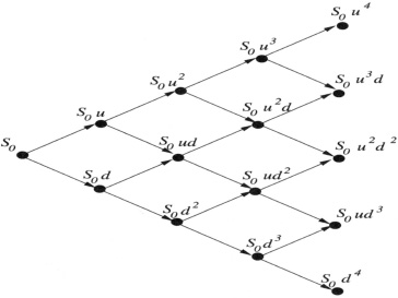
Figure 12.2   Binomial tree for N = 4

The fundamental assumption of the binomial model is that the price of the stock may take one of the two values at the expiration date. Either it will be uS₀ with probability p or it will be dS₀ with probability q = 1 − p where 0 < d < u. If there is a risk-free asset with interest rate r, as we remarked earlier, we assume that 0 < d < 1 + r < u to avoid arbitrage opportunities in the market model.

The objective is to find a strategy φ = (α₁, β₁) where such that

where R₁ = (1 + r) and S₁ = S₀ζ₁ with

P(ζ₁ = u)    =    p
P(ζ₁ = d)    =    q

such that p + q + 1.

The European contingent claim H takes two positive values H^u and H^d respectively when ζ₁ = u and ζ₁ = d:

Solving the above system of equations for the two unknowns (α₁, β₁), we get:

Set:

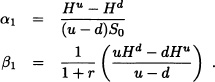
Then the initial wealth required to finance a strategy which results in values H^u and H^d is given by

where EQ(·) denotes the expectation with respect to the measure Q = (p*, q*). The initial wealth V₀ is also known as the manufacturing cost of the contingent claim. The measure Q = (p*, q*) is called the risk-neutral probability. The above equation suggests that the value of the European contingent claim is a discounted expectation of the final value under the probability measure Q. Hence it is called a risk-neutral valuation. Here we wish to note that the actual probabilities of the stock price do not appear in the valuation formula of the European contingent claim.

Note 12.4  An investor could be classified according to his preference for risk taking:

1. An investor who prefers to take the expected value of a payoff to the random payoff is said to be risk averse.
2. An investor who prefers the random payoff to the expected payoff is said to be risk preferring.
3. An investor who is neither risk averse nor risk preferring is said to be risk-neutral.

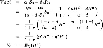
Theorem 12.9  The discounted stock price process {(1 + r)⁻ⁿS_n; n = 0,1, … , N} is a martingale under measure Q.

Proof:    Since

we have:

Thus we proved that {(1 + r)⁻ⁿS_n; n = 0,1, … , N} is a martingale under measure Q.          

12.2.2    Multi-Period Binomial Model

We now extend a one-period binomial model to an N-period model. The state space Ω = {u, d}^N is such that the elements of Ω are N-tuples with {u, d}.

For 1 ≤ n < N, we now show that there is a replication strategy for a European contingent claim H. Let φ = {(α_n, β_n): n = 1, … , N} such that:

Let V_N = H where H is an -measurable random variable. Consider the time period (N − 1, N] by using a single period model as before. We obtain

and

where Q is the risk-neutral measure.

We can find a trading strategy φ = {(α_n, β_n) : n = 1, … , N} with value process V_n(φ) such that V_N = H. We do this by working backward through the binomial tree.

For n = 1,2, … , N − 1, we assume that the self-financing strategies {(α_n, β_n) n = 1, … , N} have been determined during the time interval (n − 1, n] with value process V₁, V₂, … , V_N−1 such that

for m = n, n + 1, … , N − 1.

Let and be the two possible values of V_n. We define

and

In particular:

  EXAMPLE 12.3

We now give an example of a multiperiod pricing formula for a European call option. We suppose as before that the stock prices in each time interval are independent and identically distributed random variables each of which goes up by a factor u with probability p or down by a factor d with probability q. We know now how to price a contingent claim in a one-period model.

A European call option has a payoff at the time of expiry N as H = max(S_N − K, 0). The value of the European call option C_n = C(S_n, n) at time 0 ≤ n < N is given by:

As we illustrated earlier in Figure 12.2 for N = 4, the pricing formula for n = 0, 1, … , N − 1, we have

where E(n) is the set of indices i for which S_nuⁱd^N−n−i > K. Notice that E(n) is possibly empty in {0, … , N − n}. Set a_n = min E(n) to get:

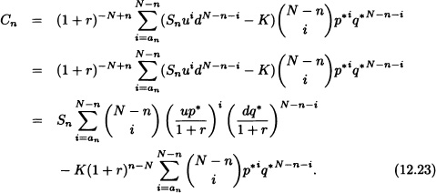
The above formula is known as the CRR formula for binomial pricing models. We observe that both sums in equation (12.23) can be expressed in terms of binomial probabilities. Let Π(k, p_u, a) be the probability that the cumulative binomial probability B(k, p_u) is larger than or equal to a with . Then equation (12.23) can be rewritten as:

Note 12.5  Let us assume that trading takes place during the interval [0, T]. We consider the stock price process introduced earlier for the fixed time interval [0, T] divided into N subintervals of equal length Δ_N with Δ_N = . We let the parameters depend on N as follows. For a given volatility of the stock, σ > 0, the step interest rate up and down factors are given by:

Assume N → ∞. At any time, the fair price of a European call option with payoff max(S^N (T) − K, 0) has the limiting value

where:

Equation (12.28) is the famous Black-Scholes formula. For more details see Bingham and Kiesel (2004).

Figure 12.3    Binary tree

  EXAMPLE 12.4

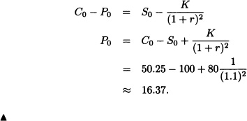
[Williams (2006), page 28]. Consider a European call option in the CRR model with N = 2, S₀ = $100 and S₁ = $200 or S₁ = $50 with strike price K = $80 and expiry date N = 2. Assume the risk-free interest rate r = 0.1.

(a) Calculate the arbitrage-free price for the European call option at time n = 0.

(b) Find the hedging strategy for this option.

(c) Suppose that the call option is initially priced $2 below the arbitrage-free price. Describe a strategy that gives an arbitrage.

(d) Using put-call parity, find the value of the European put option at time n = 0.

Solution: We have N = 2, S₀ = $100, u = 2, d = , r = 0.1 and K = $80. We calculate the risk-neutral probability

The binary tree for the stock price is given in Figure 12.3.

(a) The possible values for European call option H = max (S₂ − K, 0) are $0, $20, $320 respectively. By using the CRR formula for the European call option, we have:

(b) Using expressions (12.20) and (12.21) we calculate

and

Hence:

(c) We suppose that the value of the call option is priced at $48.25. Then one can buy the option at $48.25 and invest $2 in the bond. At time N = 2, he earns the profit of $2(1.1)² = $2.42 > 0, which gives an arbitrage opportunity.

(d) The value of the put option is calculated from (a) using put-call parity:

Note 12.6  Now we will explain briefly how to use a CRR binomial tree to value American options. The interested reader may refer to Bingham and Kiesel (2004) or Williams (2006).

An American contingent claim X is represented by a sequence of random variables X = {X_n; n = 0,1, …, N} such that X_n is -measurable for n = 0,1, … , N. For the American call option on the stock S with strike price K, X_n = max(S_n − K, 0). To define the price of the contingent claim associated with {X_n;n = 0,1, … ,N}, we proceed with backward induction starting at time N. Let U_m be the minimum amount of money required for the writer of the American contingent claim at time m to cover the payoff at time N if a buyer decides to claim at time 0 ≤ m ≤ N. The time m is a random variable and is also known as a stopping time.

A self-financing strategy is called a super hedging for the writer if φ = {(α_n, β_n); n = 1,2, … , N} with value V_n(φ) at time n such that U_n ≤ V_n(φ) for n = 0,1, … , N. We assume that U_N = X_N. The minimum amount of money required at time N − 1 to cover the payoff of the American contingent claim at time N is:

But in the case of the holder exercising his right at time N − 1, he will earn X_N−1. Hence the value of the American contingent claim at time N − 1 is:

By induction, we can see that the value of the American contingent claim for n = 1, 2, … , N is:

12.3    CONTINUOUS-TIME MODELS

We will discuss the continuous-time modeling of financial derivatives. We consider a finite time interval [0,T] for 0 < T < ∞. The continuous-time market modeled by a probability space and a filtration is the standard filtration generated by a Brownian motion . As in the case of discrete-time, we consider a financial market consisting of a risky asset, namely a stock with price process and a risk-free asset with price process . As suggested by Black-Scholes (1973), we assume that the behavior of the strike price is determined by the stochastic differential equation

where μ and σ are two constants and B_t is a Brownian motion. We also assume that a bond is risk-free, which yields interest at rate r, where the constant r is the continuously compounding rate of return. The price dynamics of the bond takes the form

The solution of equations (12.30) and (12.31) are easily computed to obtain

and

for 0 ≤ t ≤ T.

Note 12.7  The stock price process described in equation (12.32) implies that the log-retuns

are normally distributed with mean (T − t) and variance σ²(T − t). The parameter σ is also called the volatility of the stock. Hence, the stock price S_t has a log-normal distribution.

We now define the trading strategy and value of the portfolio process for the continuous-time models.

Definition 12.14  A trading strategy is a stochastic process φ = {φ_t = (α_t, β_t) : 0 ≤ t ≤ T} satisfying the following conditions:

1. -measurable where φ(t,ω) = φ_t(ω) for each 0 ≤ t ≤ T and .
2. φ_t is -adapted for each 0 ≤ t ≤ T.
3. a.s.

As before α_t and β_t represent the number of units of shares and bonds respectively.

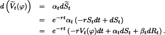
The value process or value of the portfolio at time t is given by:

In the discrete-time models we have seen self-financing strategies. Similarly the trading strategy φ is called a self-financing strategy if

for all 0 ≤ t ≤ T, or equivalently

for all 0 ≤ t ≤ T.

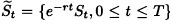
Now we define discounted price processes for the stock and value processes. The discounted stock price process is given by

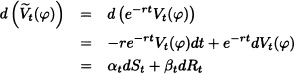
and the discounted value process is given by

By use of Itô’s formula:

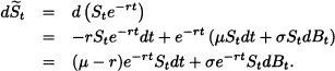
Thus:

In integral form this is

since

Theorem 12.10  A trading strategy φ is self-financing if and only if the discounted process can be expressed for all t [0, T] as:

Proof:  We know that

so that:

Hence

for 0 ≤ t ≤ T. Conversely suppose that (12.34) holds. Then

Again by Itô’s formula

and hence φ is a self-financing strategy.          

Definition 12.15  A self-financing strategy φ is called an arbitrage opportunity if

We now introduce an equivalent martingale measure.

Definition 12.16  A probability measure Q is called an equivalent martingale measure or risk-neutral measure if:

1. Q is equivalent to measure P.
2. The discounted stock price process is a martingale under measure Q, i.e., for all 0 ≤ t ≤ T.

We now give the valuation formula for a European contingent claim under a risk-neutral measure.

Theorem 12.11  Consider a European contingent claim H which is a measurable random variable such that E_Q (|H|) < ∞. Then the fair price or arbitrage-free price for the European contingent claim H at time t equals:

Proof:  Let us assume that there exists an admissible trading strategy φ = {(α_t, β_t); 0 ≤ t ≤ T} that replicates a European contingent claim. Then the value of the replicating portfolio at time t is:

The discounted value process at time t is:

Since no funds are added or removed from the replicating portfolio and the portfolio is self-financing, by Theorem 12.10 we can write the portfolio as:

Also H can be replicated by self-financing strategy φ and the value process {V_t; t ≥ 0}.

We have H = V_T and hence:

Now let be a martingale under measure Q. We have:

Hence:

Therefore:

          

12.3.1    Black-Scholes Formula European Call Option

In this section we derive Black-Scholes formula for European call option using two different approaches. In the first approach we apply the results of the risk-neutral measure for a European call option.

Let us consider a European call option on a stock with strike price K. The claim has a payoff function H = max(S_T − K, 0) at expiry time T. The strike price follows the geometric Brownian motion

where and σ > 0.

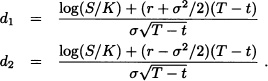
Theorem 12.12  Suppose that the stock follows the geometric Brownian motion described above with strike price К and expiry date T. Then the value of the European call option at time t is given by

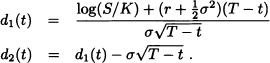
where

where Φ(.) is the cumulative normal distribution and r is the risk-neutral interest rate.

Proof:  We know that S_t satisfies the equation

where B_t is a Brownian motion. Thus S_t is of the form

where S₀ is the price of the stock at time t = 0.

Under a risk-neutral measure the fair price of the call option is:

Without loss of generality, we assume that t = 0. We have:

First we evaluate the term (II). We have:

But we know that, under measure Q, and Q(Z > x) = Q(Z < −x). Hence

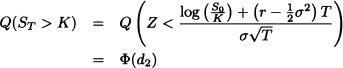
where

Now we compute the term (I):

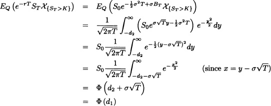
where:

Thus for any 0 ≤ t < T we have

where d₁ and d₂ are given in equations (12.36) and (12.37).        

We will prove the previous theorem by the partial differential equation approach proposed by Black-Scholes (1973). We consider the stock price process that follows geometric Brownian motion

where and σ > 0 and B_t is a Brownian motion. Consider a portfolio at time t which consists of α_t shares on stock and B_t units of bonds with value R_t. The bond is assumed to be risk-free with deterministic equation

where r > 0 is the interest rate. At time t, the value of the portfolio is:

The portfolio is supposed to hedge a European call option with value C_t = C(S_t, t). The European call option with strike price K and expiry date T has pay-off value C_t = max (S_T − K, 0). Prom Itô’s formula for the call option C, we have:

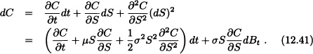
The value of the porfolio satisfies:

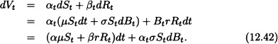
Under a self-financing strategy, equation (12.42) must coincide with equation (12.41). Since terms dt and dB_t are independent, the respective coefficients must be equal. Otherwise there shall be an arbitrage opportunity. Therefore:

From (12.45), we have:

Substituting (12.46) in (12.43), we have:

Again substituting equations (12.46) and (12.47) in (12.44), we get:

Thus we have shown that the value of a call option satisfies the above partial differential equation. This equation is also known as the Black-Scholes equation, which can be solved under appropriate conditions. Equation (12.48) can be solved for the final condition

C_T = C(S_T, T) = max (S_T − K, 0)

along with the boundary conditions

C(0, t) 0 and C(S, t) → S as S → ∞.

Finding the solution of equation (12.48) is a long computational procedure and the reader may refer to Wilmott et al. (1995). The solution of (12.48) for the value of a European call option at time T with strike price K, underlying stock price S, risk-free interest rate r and volatility σ starting from time t is given as

where:

  EXAMPLE 12.5

Consider a European call option with strike price $105 and three months to expiry. The stock price is $110 and risk-free interest rate is 8% per year, and the volatility is 25% per year.

Thus we have S₀ = 110, K = 105, T = 0.25, r = 0.08 and σ = 0.25. From equations (12.36) and (12.37) we get:

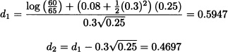
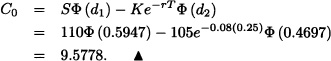
The value of the European call option calculated by using the Black- Scholes formula (12.35) is:

12.3.2    Properties of Black-Scholes Formula

The option pricing formula depends on five parameters, namely S, K, T, r and σ. It is important to analyze the change or variations of option price with respect to these parameters. These variations are known as Greek-letter measures or simply Greeks. We now give a brief description of these measures.

Delta

The delta of a European call option is the rate of change of its value with respect to the underlying asset price:

Since 0 < Φ(d₁) < 1, it follows that Δ > 0, and hence the value of a European call option is always increasing as the underlying asset price increases.

Using the information from Example 12.5, Δ = 0.724, which means that the call price will increase (decrease) with about $0,724 if the underlying asset increases (decreases) by one dollar. The delta of the put option is also given by the option’s first derivative with respect to the underlying asset price. The delta of the put option is given by:

Gamma: The Convexity Factor

The gamma (Γ) of a derivative is the sensitivity of Δ with respect to S:

The concept of gamma is important when the hedged portfolio cannot be adjusted continuously in time according to Δ(S(t)). If gamma is small, then delta changes only slowly and adjustments in the hedge ratio need only be made infrequently. However, if gamma is large, then the hedge ratio delta is highly sensitive to changes in the price of the underlying security. According to the Black-Scholes formula, we have:

Notice that Γ > 0 so that the Black-Scholes formula is always concave up with respect to S. Note the relation of a delta hedged portfolio to the option price due to concavity. The call and put options have the same gamma. For Example 12.5, the gamma for the European call option is Γ = 0.0243, which means that the rise (fall) in the underlying asset price by one dollar yields a change in the delta from 0.724 to 0.724+0.0243 = 0.7476 (0.6990).

Theta: The Time Decay Factor

The theta () of a European claim with value function C(S_t, t) is defined as:

By defining the rate of change with respect to the real time, the theta of a claim is sometimes referred to as the time decay of the claim. For a European call option on a non-dividend-paying stock:

Note that for a European call option is negative, so that the value of a European call option is a decreasing function of time. Theta does not act like a hedging parameter as is the case for delta and gamma. This is because although there is some uncertainty about the future stock price, there is no uncertainty about the passage of time. It does not make sense to hedge against the passage of time on an option.

Rho: The Interest Rate Factor

The rho (ρ) of a financial derivative is the rate of change of the value of the financial derivative with respect to the interest rate. It measures the sensitivity of the value of the financial derivative to interest rates. For a European call option on a non-dividend paying stock,

We see that ρ is always positive. An increase in the risk-free interest rate means a corresponding increase in the derivative.

Vega: The Volatility Factor

The Vega (v) of a financial derivative is the rate of change of value of the derivative with respect to the volatility of the underlying asset. Here we wish to note that vega is not the name of any Greek letters, while the names of other options sensitivities have corresponding Greek letters. For a European call option on a non-dividend-paying stock,

so that the vega is always positive and is identical for call and put options. An increase in the volatility will lead to an increase in the call option value. See Hull (2009) for more details.

Note 12.8  We wish to note that the Black-Scholes partial differential equation can also be written as:

12.4    VOLATILITY

We have seen that the Black-Scholes formula does not depend on the drift parameter μ of the stock and depends only on the parameter σ, the volatility that appears in the formula. In order to use the Black-Scholes formula, one must know the value of the parameter a of the underlying stock. We end this chapter by giving a brief description of how to estimate the volatility of stock. The volatility is a crucial component for pricing finance derivatives and estimating the value σ is the subject of study in financial statistics. One method to estimate volatility is the historical volatility whose estimates require the use of appropriate statistical estimators, usually an estimator of variance. One of the main problems in this regard is to select the sample size, or the number of observations that will be used to estimate σ Different observations tend to give different volatility estimates.

To estimate the volatility of a stock price empirically, the stock price is observed at regular intervals, such as every day, every week or every month. Define:

1. The number of observations n + 1
2. S_i, i = 0, 1, 2, 3, … , n, the stock price at the end of the ith interval
3. τ, the length of each time interval (in years).

Let

for i = 1, 2, 3, … be the increment of the logarithms of the stock prices. We are assuming that the stock price acts as a geometric Brownian motion, so that In(S_i) − In(S_i−1) ~ N(rr, σ²_T).

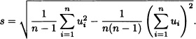
Since is the continuously compounded return (not annualized) in the ith interval. Then the usual estimate s of the standard deviation of the u_i s given by

where ū is the mean of the μ_i’s. Sometimes it is more convenient to use the equivalent formula

As usual, we assume the stock price varies as a geometric Brownian motion. That means that the logarithm of the stock price is a Brownian motion with the same drift and in the period of time τ would have a variance σ²τ. Therefore, s is an estimate of It follows that σ can be estimated as:

Choosing an appropriate value for n is not easy because σ does change over time and data that are too old may not be relevant for the present or the future. A compromise that seems to work reasonably well is to use closing prices from daily data over the most recent 90 to 180 days. Empirical research indicates that only trading days should be used, so days when the exchange is closed should be ignored for the purposes of the volatility calculation.

Another method is known as implied volatility, which is the numerical value of the volatility parameter that makes the market price of an option equal to the value from the Black-Scholes formula. We have known that it is not possible to ”invert” the Black-Scholes formula to explicitly express σ as a function of the other parameters. Therefore, one can use numerical techniques such as the bisection method or Newton-Raphson method to solve for σ. The efficient method is to use the Newton-Raphson method, which is an iterative method to solve the equation

f(σ, S, K, r, T − t) − C = 0,

where C is the market price of an option and f (.) is a pricing model that depends on σ. From an initial guess of σ₀, the iteration function is:

σ_i+1 = σ_i − f(σ_i)/(df(σ_i)/dσ).

This means that one has to differentiate the Black-Scholes formula with respect to σ. This derivative is known as vega. A formula for nu for a European call option is

With the help of software such as MATlab or Matematica one can solve the above equation. Implied volatility is a “forward-looking” estimation technique, in contrast to the “backward-looking” historical volatility. That is, it incorporates the market’s expectations about the prices of securities and their derivatives. In general volatility need not be a constant and could depend on the price of the underlying stock. These models are known as stochastic volatility models. As we stated in the introduction, we presented only a simple modeling approach for mathematical finance. Interested readers are advised to take a proper course on stochastic analysis which will take them to a more formal theory of mathematical finance, (see Williams (2006), Bingham and Kiesel (2004), and Lamberton and Lapeyre (1996).

EXERCISES

12.1    If a stock sells for $100, the value of the call option is $6, the value of the put option is $4 and both options have the same strike price, $100, what is the risk-free interest rate.

12.2    Suppose that an investor buys a European call option on certain underlying stock ABC with a $75 strike price and sells a European put option on ABC with the same strike price. Both options will expire in 3 months. Describe the investor position.

12.3    Suppose that a stock price is $120 and in the next year it will either be up by 10% or fall by 20%. The risk-free interest rate is 6% per year. A European call option on this stock has a strike price of $130. Find the probability that the stock price will rise and also the value of a call option.

12.4    Consider a European call option with 6 months to expiration. The underlying stock price is $100, strike price is $100, the risk-free interest rate is 6% and volatility is 30%. Find the risk-neutral probability and the value of the European call option using the CRR binomial model for N = 4.

12.5    Consider an American put option with 6 months to expiration. The underlying stock price is $100, the strike price is $95, the risk-free interest rate is 8% and the volatility is 30%. Find the value of the American put option at n = 0 using the CRR binomial model for N = 5.

12.6    Consider a one-period binomial model with S₀ = $40, S₁ = $44 or S₁ = $36, K = 42. The risk-free interest rate r = 12%. Find the risk-neutral probability and calculate the value of the three-month European call option

12.7    (Williams, 2006) Consider the CRR binomial model for N = 3 with S₀ = $50, u = 2, d = and risk-free interest rate r = 7%. The value of the European contingent claim at time N = 3 is given by:

K = max (S₀, S₁, S₂, S₃).

a) Find the arbitrage-free initial price of the European call option at time n = 0.

b) Determine the hedging strategy for this option.

c) Suppose that the option in (12.7) is initially priced $2 below the arbitrage- free price. Describe a strategy that gives an arbitrage.

12.8    As one increases the strike price K (keeping all other parameters fixed), does the value of a call option increase? Briefly justify your answer.

12.9    Find the expression for the delta of the put option.

12.10    Assume single-period binomial model with S₀ = $10, S_u = 12, S_d = 9 and r = 0.5. A call option on this stock has an expiry date 5 months from today and a strike price of $10. Find the value of this option.

12.11    Consider a two-period CRR model with N = 2, S₀ = $40 and strike price K = $42. In each of the next 3-month periods, the stock is expected to go up by 10% or down by 10%. The risk-free interest rate is 10% per year.

a) What is the value of a 6-month European put option?

b) What is the value of a 6-month American put option?

12.12    Consider a European call option with expiry date t = n and strike price K. Let C₀ denote its price at time t = 0. Argue that C₀ ≤ S₀; the price of any such option is always less than or equal to the price of the stock at time t = 0.

12.13    Use the Black-Scholes formula to price a European call option for a stock whose price today is $20 with expiry date 6 months from now, strike price $22 and volatility 20%. The risk-free interest is 5% per year. Find the value of the call option halfway to expiry if the stock price at that time is $21.

12.14    Use the Black-Scholes formula to price a European call option for a stock whose price today is $75 with expiry date 3 months from now, strike price $70 and volatility 20%. The risk-free interest is 7% per year.

a) Find the value of the European call option and compute delta and gamma for this option.

b) Find the value of the European put option and compute delta and gamma for this option.

12.15    Let r denote the risk-free (annual nominal) interest rate. Suppose that we consider the stock under its risk-neutral measure, that is, when μ is replaced by μ^* = r− σ²/2. Show that the expected rate of return now is r, the same as the risk-free interest rate. Explain why this makes sense.

12.16    Suppose that the observations on a stock price (in dollars) at the end of each of 15 consecutive weeks are as follows: 100.50, 102, 101.25, 101, 100.25, 100.75, 100.65, 105, 104.75, 102, 103.5, 102.5, 103.25, 104.5, 104.25. Estimate the stock price volatility.

12.17    Suppose that a call option on an underlying stock S₀ = 36.12 that pays no dividends for 6 months has a strike price of $35 with market price of $2.15 and expiry date of 7 weeks. The risk-free interest rate r = 7%. Find the implied volatility of this stock?

12.18    A call option on a non-dividend paying stock has a market price of $2.50. The stock price is $15, the exercise price is $13, the time to maturity is 3 months and the risk-free interest rate is 5% per annum. What is the implied volatility?