8
Predictive Control for Nonlinear Systems
Predictive control algorithms were firstly proposed for linear systems. The predictive control algorithms that appeared early on, such as DMC, MAC, GPC, etc. are all based on linear models, where the future outputs are predicted according to the proportion and superposition properties of linear systems. If the plant is weakly nonlinear, it can be approximated by a linear model and the linear predictive control algorithm can be used. In this case, the degeneration of the system performance caused by model mismatch due to nonlinearity is not critical and can be compensated to some extent by introducing appropriate feedback correction. However, if the plant is strongly nonlinear, the output prediction by using a linear model may lead to a large deviation from the actual one and thus the control result may be far from that predicted with the linear model. This means that it cannot be simply handled by using the linear predictive control algorithm. For predictive control applications, how to develop efficient predictive control strategies and algorithms with respect to the characteristics of nonlinear systems has always been the focus of attention. In this chapter, we firstly give the general description of predictive control for nonlinear systems and then introduce some representative strategies and methods. The predictive control algorithms for nonlinear systems are not unified and exhibit a trend of diversification according to different types of plants and different methods or tools. Therefore the main focus will be put on illustrating the specific difficulties faced by predictive control when the plant is nonlinear and the corresponding ideas to solve them.
8.1 General Description of Predictive Control for Nonlinear Systems
The basic principles of predictive control presented in Section 1.2 are also suitable for nonlinear systems. In the following, the predictive control problem for nonlinear systems is explored, starting from these principles.
The model for a nonlinear plant is usually given by one of the following two forms.
- State space model
where x ∈ Rn, u ∈ Rm, y ∈ Rp. With this model, at the sampling time k, the future state x and output y can be predicted if the initial state x(k) and the future control input u(k), u(k + 1), … are known
Starting from i = 1, by using (8.2) recursively, it follows that
where Fi(⋅) is a nonlinear function compounded by f(⋅) and g(⋅).
- Input–output model
where u ∈ Rm, y ∈ Rp and r is the model horizon. With this model, at the sampling time k, the future output y can be predicted if y(k), y(k − 1), … , u(k − 1), u(k − 2), … and the future control input u(k), u(k + 1), … are known:
Starting from i = 1 and by using (8.5) recursively, it follows that
where Gi(⋅) is a nonlinear function compounded by f(⋅).


Through step‐by‐step substitution with the model prediction formulae (8.2) or (8.5), (8.3) or (8.6) can be obtained, respectively. They both explicitly show how the system future outputs are related to the known information and future control inputs, and seem to be mostly suitable as the prediction model of the nonlinear system. However, note that the nonlinear function Fi(⋅) or Gi(⋅) needs to be multiple compounded, if f(⋅) or g(⋅) is nonlinear, and the expression of Fi(⋅) or Gi(⋅) may become very complicated when i increases. Furthermore, when solving the optimization problem, multiple compound derivatives are involved, which may be difficult to be deduced and used even if the analytic expressions of Fi(⋅) or Gi(⋅) have been obtained. Therefore, (8.3) or (8.6) can only express the prediction model in principle, and it is practically not necessary to derive Fi(⋅) or Gi(⋅). The prediction model should be directly expressed by (8.2) or (8.5) over the whole prediction horizon.
According to the principles of predictive control, at each time of rolling optimization, the actual system output should be measured and then used for feedback correction. Denote the actual output measured at time k as y(k), construct the prediction error
and then predict the future errors according to historical prediction errors e(k), …, e(k − q),
which can be used to correct the future system outputs predicted based on the model. In (8.7b) Ei(⋅) is a linear or nonlinear function, depending on the adopted noncausal prediction method and q is the time length of used historical information. Then the closed‐loop output prediction can be given by
The rolling optimization at the sampling time k is formulated as solving M control inputs starting from the current time u(k), …, u(k + M − 1) (similarly assume that u remains unchanged after time k + M − 1), which minimize the following performance index:
with

where w(k + i) is the desired output at time k + i and M and P are the control horizon and the optimization horizon, respectively. Note that ![]() in
in ![]() is obtained from the model output
is obtained from the model output ![]() given by (8.2) or (8.5) under u(k + i) = u(k + M − 1), i ≥ M, and then through feedback correction (8.8). Then the online optimization problem can be completely expressed as
given by (8.2) or (8.5) under u(k + i) = u(k + M − 1), i ≥ M, and then through feedback correction (8.8). Then the online optimization problem can be completely expressed as

If constraints on input, output, or state are concerned, they should be put into the optimization problem as a whole. After the optimal u*(k), …, u*(k + M − 1) have been solved, implement u*(k) at time k. At the next sampling time, after measuring the actual output and making a feedback correction, the optimization is repeatedly solved. This is the general description of the predictive control problem for nonlinear systems.
It can be seen that the predictive control for nonlinear systems is in principle not different from that for linear systems. However, with respect to specific algorithms, the following two aspects should be emphasized as compared with that for linear systems.
- With the prediction model of nonlinear systems, (8.2) or (8.5), it is often difficult to explicitly express the output prediction at time k in a simple analytical form of known information and assumed future control inputs. Although it is in principle possible to obtain (8.3) or (8.6) through substitution step by step, as mentioned above, such an analytical form is hard to obtain due to the nonlinear properties of f(⋅) and g(⋅). Even if it can be obtained, its multiple compounded complex form is not suitable for solving the optimization problem. Therefore, for model prediction, it is not necessary to derive a model of the form (8.3) or (8.6); instead the prediction model (8.2) or (8.5) will be established for all sampling times over the optimization horizon and taken as the constraints into the optimization problem (8.9).
- The difficulty of solving the online optimization problem in predictive control is greatly increased for nonlinear systems. Even when the performance index in (8.9) is quadratic and no constraints on input, output, and state exist, the online optimization is still a general nonlinear optimization problem because the prediction model is included in it as general nonlinear constraints. Since the optimization variables u(k), …, u(k + M − 1) appearing in the prediction models are compounded from each other, it is difficult to solve them in an analytical way, and the solution can only be obtained through numerical optimization. Due to the essential difficulty caused by the compounded nonlinearity, the solving methods, either based on parameter optimization or on function optimization, are always complicated and the computational burden is very large, which makes it difficult to meet the requirement on real‐time control. Therefore, how to efficiently solve the nonlinear rolling horizon optimization problem in real time is a difficult problem to be solved in predictive control for nonlinear systems.
In summary, although the predictive control problem for nonlinear systems can be described using a clear mathematical formulation, to solve it there still exist essential difficulties caused by nonlinearity. For decades, while predictive control for linear systems has been continually developed, much effort was also put into the research on predictive control for nonlinear systems. In addition to the theoretical research on nonlinear model predictive control (NMPC), many effective strategies and methods were proposed to meet the requirements in applications and successfully used to many real plants such as reactor, industrial robot, etc. The critical issue of these methods is how to overcome the difficulty of solving nonlinear rolling horizon optimization problems. Some of the main strategies and methods are listed as follows.
- Linearization. After linearizing the nonlinear model, design the controller using the rolling optimization method of predictive control for linear systems, while retaining the nonlinear model for prediction. To overcome the error caused by model linearization, the linearized model should be adjusted through online estimation.
- Combination of numerical computation and analytics. Use the nonlinear model for simulation to give a corresponding performance index, search the gradient direction for improving the solution through perturbing the control input, and solve the nonlinear optimization problem through repeated iteration using the gradient method.
- Layered optimization. Transform the predictive control problem for nonlinear systems into that for linear systems through feedback linearization or construct a two‐layer hierarchical algorithm; for example, decompose the global optimization problem into several small ones and at the lower layer solve small‐scale optimization problems for linearized or nonlinear models while at the high layer coordinate the interactive nonlinear items between sub‐problems.
- Multiple model. Linearize the nonlinear model at different working points and obtain multiple linear models and then use linear predictive control methods. For model selection, both switching mode and fuzzy mode are investigated. With the switching mode, determine online the adopted prediction model according to the actual state. With the fuzzy mode, synthesize online a linear model by determining the membership of the latest input/output data belonging to each linear model. This method also allows a direct start from the input/output data without the nonlinear model (8.1).
- Neural networks. Use a neural network to replace the nonlinear system model for prediction and/or design a neural network to solve the online optimization problem.
- Approximation. Approximate the nonlinear model by using a generalized convolution model or a generalized orthogonal function, etc. and solve the linear or simple nonlinear predictive control problem after truncation.
- Strategies for specific nonlinear systems, such as predictive control algorithms for the Hammerstein model, bilinear model, etc.
In the following sections, some of above predictive control strategies and methods for nonlinear systems will be introduced, aiming at meeting the requirements of predictive control applications. It should be pointed out that since the 1990s the rapid development of qualitative synthesis theory of predictive control has opened a new perspective for NMPC. Various design methods with guaranteed stability appeared in the literature. These methods focus on ensuring that the controlled system is stable and the online optimization problem involved is quite different from the one presented above, both in formulation and in the solving method. This has been partly shown in Chapters 6 and 7 and therefore will not be discussed further in this chapter.
8.2 Predictive Control for Nonlinear Systems Based on Input–Output Linearization
The control theory for nonlinear systems has achieved great progress, especially the results on feedback linearization, which have been widely used in controlling nonlinear systems. Feedback linearization refers to the introduction of nonlinear state feedback to make the closed‐loop system linear or approximately linear. With this concept it is possible to control a nonlinear system using a layered strategy, i.e. firstly to design a nonlinear state feedback control law to get a linearized closed‐loop system according to the feedback linearization theory and then to design the required controller with the help of linear control theory for the resultant system. With this layered structure predictive control for nonlinear systems can be transformed into predictive control for linear systems. In the following this layered predictive control strategy is illustrated using input–output linearization for affine nonlinear systems as an example [1].
Consider a multi‐input multi‐output affine nonlinear system:
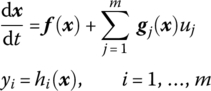
where f = (f1 ⋯ fn)T, f, gj : Rn → Rn is a smooth vector field in Rn and hi : Rn → R is a smooth scalar function in Rn, u = (u1 ⋯ um)T ∈ Rm, y = (y1 ⋯ ym)T ∈ Rm, i.e. the input and the output have the same dimension.
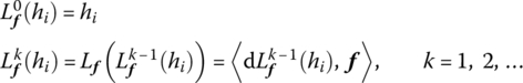
The basic idea of input–output linearization is to differentiate the output function yi successively until the input uj appears and then to design the state feedback law to cancel the nonlinear terms. To do that, the Lie derivative of hi to f is first defined:
It can be seen that Lf(hi) is just the directional derivative of hi along the vector f. It is also a scalar function in Rn. High‐order Lie derivatives can be similarly defined and expressed using the following recursive form:
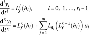
For each output component yi of the multivariable system (8.10), its relative degree ri can be defined, satisfying

According to (8.10), the first‐order derivative of yi can be written as

If ![]() , then dyi/dt = Lf(hi) has nothing with uj. Continue to find the second derivative of yi:
, then dyi/dt = Lf(hi) has nothing with uj. Continue to find the second derivative of yi:

If ![]() , then
, then ![]() has nothing with uj. Continue this procedure until
has nothing with uj. Continue this procedure until

According to the definition of relative degree ri, the second term on the right‐hand side is generally nonzero. Summarizing the results of the above steps, we get
Denote v = (v1 ⋯ vm)T, where

and βil is a positive number and can be used to assign the desired system dynamics of the linearized system. Rewrite (8.15) into the vector form
where

If the n × n dimensional matrix F(x) is nonsingular, a state feedback law can be obtained according to the above formulae:
Using this feedback law, combine (8.14) and (8.15). It follows that

In this way, the original nonlinear system (8.10) can be transformed into m decoupled single‐input single‐output linear systems (8.18) with vi as the input and yi as the output.
In the layered control structure, based on input–output linearization realized at the first layer, predictive controllers are designed at the second layer for m decoupled single‐input single‐output linear systems. For the ith subsystem (8.18), its transfer function has the form

Sampling and holding with period T, its discrete transfer function is given by

Then the GPC algorithm presented in Section 2.2 can be used to realize model prediction, rolling optimization, and feedback correction. It is also possible to calculate the coefficients of the step response from vi to yi according to this discrete transfer function and then use the DMC algorithm in Section 2.1. Specific algorithms can be referred to Chapter 2 and are no longer detailed here.
The input–output linearization‐based predictive control strategy for nonlinear systems presented above can be illustrated by the control structure shown in Figure 8.1.

Figure 8.1 Predictive control for nonlinear systems based on input–output linearization.
In the following, an example is given to illustrate the application of the presented predictive control strategy.

Figure 8.2 Planar two‐link manipulator.
In the following, an input–output linearization is first made for this system.
For h1(x), calculate


Thus we know that r1 = 2. Similarly calculate


It then follows that r2 = 2. Select the parameters of two decoupled subsystems after input–output linearization:
Substitute them into (8.16), which gives

Thus the state feedback law according to (8.17) can be calculated as

Substitute the expressions of f2(x), f4(x) into the above and the state feedback law is finally given by

With the above state feedback law, the original nonlinear system is transformed into two input–output decoupled subsystems:
The corresponding discrete input–output model with the sampling period T is given by

After feedback linearization, the problem of predictive control for the original nonlinear system is transformed into designing predictive controllers for two input–output decoupled single variable linear systems. Take T = 0.1s, using the GPC design method presented in Section 2.2, and select N1 = 1, N2 = 4, NU = 1, λ = 0.05. The control results are shown in Figure 8.3.
Figure 8.3 GPC control results of Example 8.1 after feedback linearization.
8.3 Multiple Model Predictive Control Based on Fuzzy Clustering
The predictive control method based on feedback linearization presented above needs to know the nonlinear system model and all the system states should be measurable. Much effort should be paid to calculate the nonlinear state feedback law. In practice, the approximate linearization method is always the simplest one for nonlinear system control, but with a single model it is difficult to accurately approximate the nonlinear system so a multiple model approach is often a better choice for approximating the nonlinear system.
The multiple model approach is based on the divide‐and‐conquer strategy, suitable to processes with strong nonlinearity and a large operating region. It divides the whole operating region into several separate regions. For each region the corresponding local linear model and controller are established and the global nonlinear system is then approximated and controlled by switching or integration of them. The multiple model strategy with the switching mode selects one local model/controller mostly close to the current system state as the current model/controller, focusing on the switching criterion and on how to ensure that the controlled system is globally stable. Since both model and controller are hard switched, the smoothness of the control will be affected. For the multiple model strategy with the integration mode, control is a weighted sum of local controller outputs, where the weight for each subcontroller is given by the fuzzy membership degree or the probability that the current state belongs to the corresponding local model. This approach can avoid the effect caused by hard switching. In this section, we introduce this kind of multiple model control for nonlinear systems [2, 3].
While the nonlinear system is being controlled by the multiple model approach, local models can be obtained by linearizing the nonlinear model at corresponding operating points. However, how many local models should be selected and how to judge the correlation of the current system state with each local model are always critical and difficult problems for the multiple model approach to deal with in real applications. For such problems, the development of fuzzy control provides a powerful tool. The multiple model in fuzzy control always works with the integration mode. It uses the divide‐and‐conquer strategy, with which the generalized input space of the system is firstly divided into several subspaces, then the dynamic behaviors of the global system in different subspaces are weighted and combined such that the system can run in a smooth way. Furthermore, this approach does not need to identify the nonlinear system model and can directly start from the process data with fuzziness, which is more important for real applications.
(1) Establishing the multiple model based on fuzzy satisfactory clustering (FSC)
The Takagi‐Sugeno (T‐S) model is the most widely used multiple model in fuzzy control. It directly uses the data samples of the process rather than its mathematical model. The basic form of the T‐S fuzzy multiple model with c rules is as follows:

where x = (x1 ⋯ xd)T is the input variable and Ai is its fuzzy set described either qualitatively or quantitatively. Mi represents the submodel of the ith rule, where yi is the output of the submodel and pij is the post‐parameter of the ith rule. Then the system output can be given by the weighted submodel outputs

where μi is the membership degree of x to the fuzzy set Ai.
To identify the structure of the T‐S multiple model, it is usually necessary to divide the input space at first and then to identify the parameters in the conclusion part. The main steps include clustering of the data sample set (i.e. to partition the data set Z into several fuzzy subsets by using some clustering algorithm), determination of the cluster number c (i.e. to determine the appropriate number of clusters, which is also the rule number of the T‐S fuzzy model), and identification of the fuzzy rules (including the membership function of the premise variable, the parameters of the conclusion part, etc.). Because of different clustering methods for data samples and different representations for submodels, a variety of T‐S model identification methods based on fuzzy clustering appeared in the literature. In the following the multiple modeling method based on FSC [3] is introduced.
Consider a multi‐input single‐output (MISO) system. Its sample set is composed of system input/output data. The jth sample is represented by zj = (φj yj)T, j = 1, … , N, where φj is the regression row vector, called a generalized input vector, which affects the system output. In general, it is composed of a previous system input/output and its dimension is d, yj is the system output and N is the total number of samples. Then the sample set can be represented by Z = [z1, … , zN], where zj ∈ Rd + 1. Then the sample set Z is divided into c clusters {Z1, … , Zc}. For each cluster Zi, denote its cluster center as vi = [vi, 1 ⋯ vi, d + 1]T ∈ Rd + 1, i = 1, … , c. The result of fuzzy clustering can be represented by the membership matrix U = [μi, j]c × N, where μi, j ∈ [0, 1] represents the degree to which the sample zj belongs to the ith cluster with center vi and satisfies

Gustafson and Kessel [4] proposed an efficient fuzzy clustering approach by using an adaptive distance measure for the clustering covariance matrix, called the GK algorithm; for more details refer to [4] or corresponding textbooks. This algorithm is insensitive to the initial values of the membership matrix and the clustering centers, i.e. different initial conditions do not greatly affect the clustering result. It is not necessary to normalize the sample data due to the use of an adaptive distance measure. Furthermore, it can detect different shapes of clusters because it is not limited to linear clustering. All the above advantages make it an effective clustering algorithm which is widely used in control, image processing, and other fields. However, similar to most other clustering algorithms, in the GK algorithm the cluster number c should be given in advance. Since the cluster number essentially depends on the degree of system nonlinearity, if not enough prior knowledge is available, in general it should be determined by using the trial‐and‐error method step by step, which will undoubtedly increase the computational burden.
To solve this problem, an FSC approach based on GK fuzzy clustering was proposed in [3]. Its basic idea is as follows. Firstly, start from a lower number of initial clusters, e.g. let c = 2. After initial clustering of the system, if the clustering result is not satisfactory, find a sample from the sample set as a new sample center vc + 1, which is mostly dissimilar to all the clustering centers v1~vc. Calculate the new membership matrix U using v1~vc + 1 as the initial clustering centers and repeat the GK algorithm to divide the system into c + 1 parts. This procedure is repeated according to the requirement on the performance index until a satisfactory performance index is reached. For the above discussed MISO system, the specific T‐S modeling procedure based on FSC is given as follows.
The above T‐S modeling algorithm based on FSC avoids determining cmax in terms of the system nonlinear characteristics, as used in usual clustering integration methods. It directly starts from c = 2 and makes the algorithm have a definite number for initial clustering. Furthermore, except for the first clustering, during the clustering process, the initialization parameters such as the membership matrix can be determined mainly according to the result of the last clustering and do not need to be calculated starting from random values. The computational efficiency is obviously increased, particularly for a data set with a great number of samples.
Using the FSC algorithm, the multiple model described by (8.22) can be obtained through off‐line determination of the clusters according to data samples, which realizes the multiple modeling for MISO systems. Based on that the multimodel predictive control algorithm for nonlinear systems can be introduced.
(2) Multiple model predictive control algorithm based on fuzzy clustering
A nonlinear multivariable system with r outputs can be decomposed into r MISO subsystems according to its output. After FSC modeling, the lth MISO subsystem is divided into cl clusters and described by cl submodels described in (8.22). In order to make the model suitable for predictive control algorithms such as DMC, GPC where control increments are adopted, the submodel in (8.22) is rewritten into increment form with the corresponding fuzzy rules

where φl is the generalized input vector of the lth MISO system, dl represents its dimension, yl is its output, ![]() is the projection of its ith clustering center
is the projection of its ith clustering center ![]() on the generalized input space, i.e. the remaining part of the vector
on the generalized input space, i.e. the remaining part of the vector ![]() after removing the output element,
after removing the output element, ![]() represents the hth parameter of the ith submodel,
represents the hth parameter of the ith submodel, ![]() represents the output of the ith submodel with respect to φl, and cl,
represents the output of the ith submodel with respect to φl, and cl, ![]() have been determined after off‐line modeling. The advantage of this increment form is that the constants
have been determined after off‐line modeling. The advantage of this increment form is that the constants ![]() in all linear models can be canceled.
in all linear models can be canceled.
During online control, at each sampling time when the lth MISO system obtains a new data sample φl, its membership to the ith cluster can be calculated by

where ![]() represents the membership of φl to the ith submodel
represents the membership of φl to the ith submodel ![]() of yl,
of yl, ![]() is the measure of the distance function of the new input vector φl to
is the measure of the distance function of the new input vector φl to ![]() , and m > 1 is a tunable parameter characterizing the degree of fuzziness of clustering
, and m > 1 is a tunable parameter characterizing the degree of fuzziness of clustering ![]() .
.
For the generalized input vector φl, after calculating its membership to each submodel by (8.27), the global model of the MISO system can be integrated by (8.23) and (8.27) as follows:

After obtaining the models represented by (8.28) for all MISO subsystems, the model of the MIMO system can be obtained by integrating them together:
Then the multivariable GPC algorithm can be adopted to design the multiple model predictive controller. The principle of the multiple model predictive control based on the above fuzzy clustering method is shown in Figure 8.4.
The multiple model predictive control algorithm based on fuzzy clustering for nonlinear systems can be summarized as follows. Firstly, use Algorithm 8.1 (FSC) off‐line with data samples to obtain the multiple model description (8.26) for each MISO subsystem, where the number of clusters cl, the cluster centers ![]() , and the submodel parameters
, and the submodel parameters ![]() are determined. Then turn to online control. At each step of control, measure the generalized input φl of each subsystem, calculate the membership
are determined. Then turn to online control. At each step of control, measure the generalized input φl of each subsystem, calculate the membership ![]() of it to the corresponding submodel by (8.27). Then obtain the parametric model of the whole multivariable system according to (8.28) and (8.29), and take it as the prediction model to perform predictive control using the conventional GPC algorithm.
of it to the corresponding submodel by (8.27). Then obtain the parametric model of the whole multivariable system according to (8.28) and (8.29), and take it as the prediction model to perform predictive control using the conventional GPC algorithm.
The data sample set is produced, from which the multiple model can be obtained using Algorithm 8.1 based on FSC. Figure 8.6a and b show the modeling results for the pH channel and the h channel, respectively, when the cluster number is six. It can be seen that for both channels the model has a good fitting degree. The RMSE for the pH channel and the h channel is 0.209 and 0.0318, respectively, which indicates that the model can well approximate the nonlinear characteristics of the system.
After obtaining the local models of two MISO systems off‐line (each has six submodels; refer to [3] for details), the global model of this multivariable system can be obtained online according to (8.27), (8.28) and (8.29). For GPC control, select the design parameters N1 = 1, N2 = 5, NU = 2, Q = 0.1I, R = 0.01I. In Figure 8.7, the variations of the control inputs and the system outputs by using the unconstrained multivariable GPC algorithm are shown for tracking pH (9 → 8 → 9 → 8) and h (15 → 17 → 16 → 18) with a constant disturbance Fbf = 0.55 ml/s. With other simulations it is also found that the system outputs exhibit good tracking performance for different disturbance amplitudes, and there is no steady‐state error if the disturbance remains constant.
The above‐introduced multiple model predictive control algorithm based on fuzzy clustering does not need the nonlinear model of the system and can directly start from the input and output data. Through fuzzy clustering, the problem of identifying a complex nonlinear system is solved by firstly finding a set of simple linear models for corresponding subregions defined by fuzzy boundaries and then establishing the system global model by integrating them through fuzzy weighting. In this way the predictive control problem for nonlinear systems can be transformed into that for linear systems, where the predictive control algorithm is not based on one of multiple models selected according to the system input/output but on the system global model integrated according to the degree of input/output belonging to each model. Thus the online switching problem can be avoided. This multiple model predictive control method has a wide selection space both in specific clustering strategies and in model forms. More algorithms and effective applications can be referred to the relevant literature.

Figure 8.4 Structure of multiple model predictive control based on fuzzy clustering [2].
Figure 8.5 pH neutralization process [3].
Source: Reproduced with permission from Ning Li, Shao‐Yuan Li and Yu‐Geng Xi of Elsevier.

Figure 8.6 Fuzzy modeling of pH neutralization process [3]: (a) pH channel, (b) h channel.
Source: Reproduced with permission from Ning Li, Shao-Yuan Li and Yu-Geng Xi of Elsevier.

Figure 8.7 Result of multiple model predictive control for pH neutralization process with constant disturbance Fbf = 0.55 ml/s [3].
Source: Reproduced with permission from Ning Li, Shao‐Yuan Li and Yu‐Geng Xi of Elsevier.
8.4 Neural Network Predictive Control
Artificial neural network provides a powerful tool for modeling and control of nonlinear systems and has been widely used in many fields. Since the 1980s, the application of neural networks in the control field has rapidly developed and a number of survey papers appeared in which the neural network predictive control is also a typical example for neural network applications [6]. The applications of neural networks in predictive control include neural network modeling for nonlinear systems and optimization solving using neural networks. In relevant literature, it is usual to adopt a neural network for modeling and then to realize the predictive control in two different ways. One is directly using a neural network to solve the rolling optimization problem, while the other is firstly to identify the system dynamic response by a neural network model and then to solve the online rolling optimization using the parametric optimization method. In this section, we briefly introduce the predictive control algorithm directly using neural networks to modeling and on‐line optimization for single‐input single‐output nonlinear systems [7].
(1) Neural network for modeling and prediction
Assume that the input–output model of a nonlinear system can be represented by
For neural network modeling, this specific representation (8.30) is unknown and only the input and output sample data are available. Consider the commonly used backpropagation (BP) network with one layer of hidden nodes. It is composed of three layers of nodes, i.e. the input node layer, the hidden node layer, and the output node layer. Nonlinear transformation is considered only in the hidden node layer. Denote the output of the input node as oj, j = 1, … , na + nb ≜ nt. They are indeed the variables in the bracket on the right side of (8.30). Denote the input of the hidden node i as xi and its output as zi, i = 1, … , m, where m is the number of hidden nodes. Denote the output of the output node as ![]() . According to the working principle of the BP network, it follows that
. According to the working principle of the BP network, it follows that

where wij is the weighting coefficient of connection from the input node j to the hidden node i, wi0 is the input bias of the hidden node i, wi is the weighting coefficient of connection from the hidden node i to output node, w0 is the input bias of the output node, and φ(⋅) is the action function of the neuron, usually taken as the Sigmoid function
The task of neural network modeling is to determine the weighting coefficients and the input biases best matched with the given sample data set, which can be described as the following optimization problem:

where N is the number of samples, yl and ![]() represent, respectively, the system output in the lth group of samples and the neural network output calculated by (8.31) of this sample, and w is a parameter vector containing all the weighting coefficients and input biases.
represent, respectively, the system output in the lth group of samples and the neural network output calculated by (8.31) of this sample, and w is a parameter vector containing all the weighting coefficients and input biases.
The weighting coefficients of the BP network can be obtained as follows. Let

then
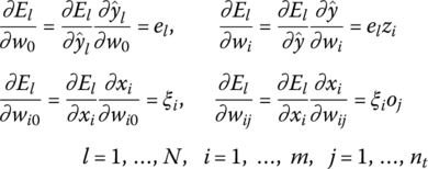
After setting the initial parameter vector w for each sample, the network output ![]() can be calculated by (8.31) for input oj and compared with the actual output yl to construct the error el. Starting from the output side, use the back propagation of error el to calculate δi, ξi using (8.34) and the partial derivative of El to w (w refers to any network parameter in w) using (8.35). Then construct
can be calculated by (8.31) for input oj and compared with the actual output yl to construct the error el. Starting from the output side, use the back propagation of error el to calculate δi, ξi using (8.34) and the partial derivative of El to w (w refers to any network parameter in w) using (8.35). Then construct

based on which the network parameters are improved by the gradient method
This process is repeated until the performance index (8.33) reaches the minimum. Then the obtained BP network is the best match to the sample data set. It implicitly establishes the nonlinear mapping (8.30) between historical data and the current output, which can be directly used to one‐step output prediction when the current control input is given.
However, in predictive control, the above neural network needs to be improved for a multistep prediction. The simplest way is to establish P simple BP networks, as above, when the prediction horizon is P, where the output of the sth BP network is the system output ![]() predicted at k, s = 1, … , P. For the sake of symbol brevity, assume na = nb ≜ n in the nonlinear model (8.30). According to (8.4) and (8.6), from (8.30) it follows that
predicted at k, s = 1, … , P. For the sake of symbol brevity, assume na = nb ≜ n in the nonlinear model (8.30). According to (8.4) and (8.6), from (8.30) it follows that
Thus the sth BP network should be an approximation of the nonlinear mapping Gs(⋅) from the input/output information available at time k and the future control inputs to ![]() . Refer to (8.31) and consider the control horizon M ≤ P; the sth BP network can then be expressed by
. Refer to (8.31) and consider the control horizon M ≤ P; the sth BP network can then be expressed by

These BP networks work using the same principle and the whole network outputs can reflect the predicted future outputs at different times over the prediction horizon. Since both the learning process and the real‐time prediction of these BP networks can be done in parallel, it is a practical and efficient way for multistep prediction for nonlinear systems.
(2) Neural network for online optimization
After establishing the neural network model for the nonlinear system, we now discuss the predictive control method based on that. Predictive control runs in a rolling style, i.e. at each sampling time the control action is obtained by online solving a nonlinear optimization problem. In addition to output prediction, the neural network model established above can also be used for online optimization, which can be solved by the same gradient optimization process as that in model parameter identification.
At the sampling time k, let the optimization performance index J(k) have the form
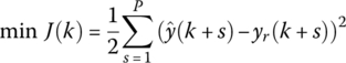
where ![]() (s = 1, … , P) are the outputs of the basic BP prediction models when future inputs are u(k + h − 1)(h = 1, … , M), yr(k + s)(s = 1, … , P) are the desired outputs. Note that
(s = 1, … , P) are the outputs of the basic BP prediction models when future inputs are u(k + h − 1)(h = 1, … , M), yr(k + s)(s = 1, … , P) are the desired outputs. Note that

and it is known from (8.38) that ![]() is not related to u(k + h − 1) when h > s, so the above equation can be rewritten into
is not related to u(k + h − 1) when h > s, so the above equation can be rewritten into

where

Furthermore, according to the performance index (8.40), it follows that

Then the gradient can be given by

Therefore, one can initially set a group of controls uM(k), calculate ![]() using the model (8.39), and then substitute it into the performance index (8.40) to calculate
using the model (8.39), and then substitute it into the performance index (8.40) to calculate ![]() in J(k). Based on that premise, the control can be improved by the gradient method
in J(k). Based on that premise, the control can be improved by the gradient method

where α is the step length and the gradient can be calculated by (8.42). This iteration process should be repeated until J(k) reaches a minimum. Then u(k) as the current optimal control can act for the system for control.
The above predictive control algorithm with neural network modeling and online optimization can be described by the internal model control (IMC) structure shown in Figure 8.8, where MNN is the one‐step neural network prediction model. It only provides the predicted model output at the next sampling time in terms of current control and (8.39), and then constructs the output error using the measured real output to make a feedback correction. The core part in the figure is the neural network online optimization controller CNN. It uses the neural network prediction model (8.39) and the optimization algorithm (8.42), (8.43) to iteratively calculate the optimal control and then implements the current control, where the weighting coefficients of the model (8.39) have been obtained through off‐line learning.
The presented algorithm is only a fundamental one of the neural network based on predictive control algorithms. In fact, there are a large variety of methods both for neural network modeling and for predictive control based on the neural network model: for example, using the Hopfield network model, considering a general nonlinear performance index instead of a quadratic one, putting constraints on the system input and output, identifying step response coefficients after establishing the neural network model and then using traditional predictive control algorithm, and so on. This can be referred to much of the literature on neural network predictive control. Later in Chapter 10, we will also introduce an application example of using the simplified dual neural network (SDNN) to solve the quadratic programming (QP) problem in predictive control and implementing the algorithm in DSP.
Figure 8.8 Structure of the neural network based predictive control for nonlinear systems.
8.5 Predictive Control for Hammerstein Systems
The nonlinearity of many systems is caused by the input component, such as input saturation, dead zone, hysteresis, etc. Among those the Hammerstein model is typical to describe the system with input nonlinearity. It is composed of a static nonlinear component and a dynamic linear component. Since a large variety of nonlinear processes such as pH neutralization, high purity separation, etc. can be described by the Hammerstein model, identification and control of such systems have been widely investigated. The control strategies for Hammerstein systems can be roughly classified into two catalogs. One is the global solving strategy, i.e. including the input nonlinear part in the optimization problem and solving the control action directly, which is of course very difficult. Another is the nonlinear separation strategy, that is, firstly using some control algorithm for the dynamic linear model to calculate its input, which is an intermediate variable but also the output of the static nonlinear component, and then conversely calculating the actual control according to the static nonlinearity. This strategy fully uses the specific structure of the Hammerstein model and transforms the controller design problem into a linear control one, and is thus much simpler than the global solving strategy.
An unconstrained single variable predictive control problem for the Hammerstein model was investigated early in the 1980s. In recent years, the research on predictive control for this kind of system is more in‐depth, including adopting different linear models and different predictive control laws, considering input saturation constraints and other input nonlinearities, and studying the stability of the closed‐loop system, etc. Here we only introduce a two‐step predictive control strategy for the Hammerstein model while considering the input saturation constraints [8, 9].
Consider the Hammerstein model composed of a memoryless static nonlinear component
and a dynamic linear component
where x ∈ Rn, v ∈ Rm, u ∈ Rm are the state, intermediate variable, and input, respectively, and Φ represents the nonlinearity between the input and intermediate variable. Assume that state x is measurable and the pair (A B) is controllable. Also assume the nonlinearity Φ = f ∘ sat, i.e. compounded by an invertible static nonlinearity f(⋅) and a physical input saturation constraint sat represented by

According to the system model given by (8.44) and (8.45), it can be found that the control input u affects system state x through intermediate variables v. Although the relationship between u and x is nonlinear, the relationship between v and x is linear. Therefore, the control law can be calculated in two steps. Firstly, the desired intermediate variable v(k) is solved by using the unconstrained predictive control algorithm for the linear model (8.45). Then the control action u(k) can be obtained by solving the nonlinear algebraic equation group (NAEG) (8.44) and the saturation constraints can be satisfied by using the desaturation method. This two‐step predictive control strategy is indeed a nonlinear separation strategy. In the following the solving procedure of this strategy is given in some detail.
Firstly, consider the predictive control problem for the linear model (8.45) with input v and state x. It is a conventional unconstrained predictive control problem. Let x(k + i ∣ k), v(k + i ∣ k) be the future state and intermediate variable at time k + i, both predicted at time k, and define the optimization performance index at time k as

where N is the optimization horizon, Q ≥ 0, R > 0 are weighting matrices of state and intermediate variables, and the terminal state weighting matrix QN > 0. At each time k, with measured state x(k), the following optimization problem should be solved:

This is a finite horizon standard LQ problem and the optimal LQ control law can be given by
where Pi can be calculated using the following Riccati iteration:

Thus, the optimal predictive control law v(k) = v(k ∣ k) can be given by
After v(k) has been solved, the task of the second step is to back‐calculate the control u(k) according to (8.44) and make it satisfy the input saturation constraint (8.46). Note that the control law (8.50) may be unable to be implemented via u(k), so the v(k) given by (8.50) is only a desired intermediate variable and is denoted as vL(k) in the following. The NAEG vL(k) − Φ(u(k)) = 0 can be solved for u(k) by iteration and there exist various methods depending on the specific form of f(⋅). In order to reduce the computational burden, it is suggested to use the Newton iteration method or its simple modified forms. Sometimes the solution of NAEG is not unique. In this case, it can be determined by additional conditions, such as choosing u(k) mostly close to u(k − 1), choosing u(k) with the smallest amplitude, etc. Thus we can get the solution of the above NAEG and formally denote it as ![]() . Then the control input u(k) can be obtained by desaturation of
. Then the control input u(k) can be obtained by desaturation of ![]() with
with ![]() such that (8.46) is satisfied.
such that (8.46) is satisfied.
The control structure of the two‐step predictive control algorithm for the Hammerstein model (8.44), (8.45) is shown in Figure 8.9.

Figure 8.9 Structure of the two step predictive control system [9].
It is obvious that when implementing u(k) = sat(g(vL(k))) ≜ (sat ∘ g)(vL(k)) on the input of the Hammerstein system, the resultant v(k) = f(u(k)) = (f ∘ sat ∘ g)(vL(k)) is in general not the same as vL(k), i.e. the control law in terms of the intermediate variable v(k) is formally given by
which is not exactly the optimal LQ control law (8.50). Under certain conditions on the LQ design parameters and on h(vL(k)) [8], some theoretical results were achieved on the stability of the closed‐loop system and on the domain of attraction.
It can be seen that for the Hammerstein system described by (8.44), (8.45), using the idea of dynamic‐static separation can divide its predictive control problem into two parts: an unconstrained predictive control problem for the linear dynamic model and an NAEG solving problem for the nonlinear static model. With the specific form of this model, the rolling optimization is actually implemented for a linear model rather than for a nonlinear one. The input nonlinearity is only handled as an additional static component. Here only some simple cases have been discussed, aiming at illustrating how the two‐step control strategy is adopted by taking advantage of such a model structure into account. In fact, for predictive control of the Hammerstein model and even for systems with more general input nonlinearity, there exist abundant research results on both strategies and theory.
8.6 Summary
Predictive control for nonlinear systems has the same principles as that for linear systems, i.e. predicting the future dynamic behavior of the system based on the prediction model, implementing real‐time control through online solving nonlinear optimization problems using model prediction, and correcting the model prediction by using real‐time measured system information. However, compared with predictive control for linear systems, deriving an explicit causal prediction model without intermediate variables becomes complicated because the proportion and superposition properties no longer hold for nonlinear systems and the nonlinearity is often complex and diverse. In this case, the fundamental nonlinear model should be established for all the time instants over the optimization horizon and put as equality constraints into the optimization problem. With respect to online optimization, even without input, output, and state constraints, the analytical solution is almost impossible to derive, and the nonlinear programming method is often needed to find the solution iteratively. Therefore, how to effectively solve the online optimization problem is the most difficult problem in predictive control for nonlinear systems. In accord with this, this chapter has been to focus on the efficient strategies and methods of predictive control for nonlinear systems.
The layered structure of predictive control for nonlinear systems can effectively utilize the mature technology of predictive control for linear systems. There exist various layered strategies in predictive control applications, such as the hierarchical predictive control for urban traffic networks to be introduced in Section 10.2.4. The predictive control based on input–output linearization presented here provides a general framework where the feedback linearization at the lower layer aims at transforming the nonlinear system into a linear one for which mature predictive control algorithms can be adopted.
The fuzzy multiple model and neural network are common tools to deal with nonlinear systems and provide a new way for its predictive control. The use of them in predictive control indicates that in addition to the predictive control based on usual mathematical models, it is also possible to make prediction and optimization directly starting from the process data through establishing a neural network model or fuzzy model. This is the concrete embodiment of the predictive control principles and provides an open space for developing new kinds of prediction model, rolling optimization, and feedback correction. It is particularly advantageous for practical use when the model identification is difficult or expensive but the process data are rich and available.
The description of nonlinear systems is much more complex than that of linear systems, which prevents the general formulation and solution of predictive control for nonlinear systems. However, for nonlinear systems with special nonlinear forms or with specific characters, it is still possible to develop effective predictive control strategies or algorithms. The Hammerstein model is a typical nonlinear system with a linear dynamic model and static input nonlinearity. The two‐step predictive control presented here makes dynamic‐static separation in terms of the specific character of the model, and thus greatly simplifies the controller design.
Predictive control for nonlinear systems has been always the focus of attention since the appearance of predictive control. In addition to fruitful results in theoretical research of NMPC, many effective algorithms and strategies were developed to meet the needs from practical applications. In this chapter, only a few of these research works were introduced. Compared with the maturity of predictive control for linear systems, predictive control for nonlinear systems is still the most challenging topic in the field of predictive control.
References
- 1 Sun, H. Layered predictive control strategies for a class of nonlinear systems. PhD thesis, 1990. Shanghai Jiao Tong University (in Chinese).
- 2 Li, N. Multi‐model‐based modeling and control. PhD thesis, 2002. Shanghai Jiao Tong University (in Chinese).
- 3 Li, N., Li, S., and Xi, Y. (2004). Multiple model predictive control based on the Takagi‐Sugeno fuzzy models: a case study. Information Sciences 165 (3–4): 247–263.
- 4 Gustafsson, D. and Kessel, W.C. Fuzzy clustering with a fuzzy covariance matrix, Proceedings of 1978 IEEE Conference on Decision and Control, San Diego (10–12 January 1979), 761–766.
- 5 Takagi, T. and Sugeno, M. (1985). Fuzzy identification of systems and its applications to modeling and control. IEEE Trans. SMC 15 (1): 116–132.
- 6 Hunt, K.J., Sbarbaro, D., Zbikowski, R. et al. (1992). Neural networks for control systems – a survey. Automatica 28 (6): 1083–1112.
- 7 Li, J., Xu, X., and Xi, Y. Artificial neural network‐based predictive control, Proceedings of IECON’91, Kobe, Japan (28 October–1 November 1991), 2: 1405–1410.
- 8 Ding, B.C., and Xi, Y.G. (2006). A two‐step predictive control design for input saturated Hammerstein systems. International Journal of Robust and Nonlinear Control 16 (7): 353–367.
- 9 Ding, B.C. Methods for stability analysis and synthesis of predictive control. PhD thesis, 2003. Shanghai Jiao Tong University (in Chinese).