7.1.1 Synthesis of RMPC Based on Ellipsoidal Invariant Sets

Many uncertain systems can be described by the following linear time varying (LTV) system with polytopic uncertainty:

(7.1)

where A(k) ∈ R^n × n, B(k) ∈ R^n × m, and

(7.2)

where Co means a convex hull, i.e. for any time‐varying A(k) and B(k), [A(k) B(k)] ∈ Π means that there exists a group of non‐negative parameters λ_l(k), l = 1, …, L satisfying

(7.3)

The uncertainty described by (7.2) and (7.3) is called polytopic uncertainty, which can be formulated by a convex hull with L given vertices [A_l B_l]. The real system parameters [A(k) B(k)] will always be in the convex hull and λ_l are the convex combination parameters, either time‐varying or time‐invariant.

The system model with polytopic uncertainty can describe both nonlinear systems which are linearized at several equilibrium points and some linear systems with time‐varying parameters. For example, the linear parameter varying (LPV) system can be formulated by (7.2) and (7.3). Therefore, much RMPC literature focuses on this kind of uncertain system.

In addition, consider the constraints on system inputs and outputs:

(7.4)

(7.5)

Note that in order to highleight the basic idea of RMPC synthesis, (7.4) and (7.5) are taken as examples of system constraints. For other kinds of constraint, such as the peak bounds on individual components of system input or output, as discussed in Section 6.1.4, the results derived here only need to be adjusted accordingly.

For this kind of uncertain system described by (7.1) to (7.3), and with input and output constraints (7.4) and (7.5), referring to the linear robust control theory, the following infinite horizon “min‐max” problem is proposed at time k:

(7.6)

Different from the optimization problem in previous chapters, the min‐max problem (7.6) results from the uncertainty of the system model. This means that the RMPC will optimize the future performance index with an infinite horizon so as to achieve an optimal solution for the worst case in all possible model variations in Π.

The min‐max problem (7.6) is a reasonable formulation of RMPC for an uncertain system (7.1) to (7.5), but is difficult to solve. Firstly, the objective of the minimization in (7.6) results from the maximization procedure and is heavily affected by system uncertainty, while the objective of the usual optimization method is explicitly given by analytical functions or variables. Secondly, the infinite terms in the objective function make the optimization computationally intractable. A specific strategy should be adopted to make the optimization problem solvable. In the following, referring to [1], we introduce the synthesis method of RMPC for this kind of polytopic uncertain system, explaining how to use an effective strategy to overcome these difficulties and how to implement it using LMIs and ellipsoidal invariant sets.

(1) Strategy and key ideas

1) Introducing an upper bound for the maximization problem Consider the quadratic function V(i, k) = x(k + i ∣ k)^TPx(k + i ∣ k), where P is a symmetric positive definite matrix. At time k, for all x(k + i ∣ k) and u(k + i ∣ k) satisfying (7.1) to (7.3), impose the following condition on the corresponding function V:

(7.7)

This condition implies that the closed‐loop system is stable. Therefore x(∞ ∣ k) = 0 and thus V(∞, k) = 0. Summing (7.7) from i = 0 to i = ∞, it follows that

Then define an upper bound γ > 0 on the robust performance index

(7.8)

In this way the min‐max problem (7.6) can be converted into a minimization problem with a simple linear objective γ.

2) Adopting a single feedback control law for the infinite horizon

In order to handle the infinite number of control actions in problem (7.6), introduce the ellipsoid controlled invariant set

(7.9)

with a corresponding state feedback control law

(7.10)

Control invariance means that if the system state x(k ∣ k) = x(k) ∈ Ω, then under the control law (7.10), x(k + 1 ∣ k) ∈ Ω. This can be ensured by

and furthermore

(7.11)

Use of the above state feedback control law and the corresponding ellipsoid controlled invariant set make it possible to parametrize the control actions to a tractable form as well as to keep the system state within the invariant set.

(2) Constraints formulated in LMIs

Using the above key ideas, the min‐max problem (7.6) can be converted into an optimization problem of minimizing the upper bound γ by using the state feedback control law (7.10) with the following constraints: the upper bound constraint (7.8), controlled invariant set conditions (7.9) and (7.11), and input/output constraints (7.4) and (7.5), where γ, P, Q, F should be determined. Note that the quadratic form of x^TPx in the upper bound constraint (7.8) is in accordance with the ellipsoid set representation in (7.9). Use P = γQ⁻¹ to reduce the complexity. Then, with the help of the Schur Complement of LMIs (6.11) and the properties of the convex hull (7.3), the details of synthesizing the RMPC can be given as follows.

1. The upper bound of the maximum of the objective function (7.8). From (7.8) it follows that
   

   With P = γQ⁻¹ and x(k ∣ k) = x(k) the above inequality is exactly the invariant set condition (7.9) and can be rewritten in LMI form as

   (7.12)

2. Imposing V(i, k) descending and satisfying (7.7). With V(i, k) = x(k + i ∣ k)^TPx(k + i ∣ k) and (7.1), (7.10), the condition (7.7) can be expressed as

   ∀[A(k + i) B(k + i)] ∈ Π, i ≥ 0

   

   This inequality can be ensured by the following matrix inequality:

   (7.13)

   With P = γQ⁻¹, left‐ and right‐multiplying Q on both sides will yield

   

   Let Y = FQ and rewrite the above matrix inequality as

   

   According to (6.11d) and (6.11e), this condition can be expressed in the following LMI form:

   

   where the symbol * is used to induce a symmetric structure of the matrix for simplicity.

   Since the uncertain parameters A(k + i) and B(k + i) satisfy the polytopic condition (7.3) and can be represented by a linear combination of parameters of the vertices [A_l B_l] in the polytopic model, the above condition is satisfied if the following group of LMIs holds:

   (7.14)

3. x (k) in the ellipsoid set Ω = {x ∈ Rⁿ ∣ x^TQ⁻¹x ≤ 1}. This is also described by (7.12) because the condition x^T(k)Q⁻¹x(k) ≤ 1 is identical to x^T(k)Px(k) ≤ γ under the selection P = γQ⁻¹ and γ > 0.
4. Ω is an invariant set of system (7.1) under the feedback control law (7.10), i.e. (7.11):
   

   It is obviously covered by the V(i, k) descending condition (7.13) with P = γQ⁻¹ and γ > 0. Thus the corresponding LMI has already been included in (7.14).

5. Constraints on control inputs (7.4). Referring to (6.13) in Section 6.1.4, it can be given by
   (7.15)

6. Constraints on system outputs (7.5). According to (7.5) and referring to (6.15) in Section 6.1.4, it follows that
   (7.16)

(3) RMPC algorithm with robust stability

Summing the above derivations, at time k, solving the min‐max problem (7.6) can be converted into solving the following optimization problem:

(7.17)

After Q and Y are solved, we can obtain F = YQ⁻¹ and u(k) = Fx(k), i.e. the current control action at time k. Note that {γ, Q, Y} are solved at time k, and strictly they should be denoted by {γ(k), Q(k), Y(k)}.

Now the RMPC algorithm based on ellipsoidal invariant set can be given as folllows.

For Algorithm 7.1, the following theorem on the stability of the closed‐loop system can be given.

The above proposed RMPC should solve the optimization problem (7.17) online by using LMIs toolboxes. The online computational burden is determined by the number of optimization variables and the number of rows of LMIs. It is easy to see that both of these two numbers will increase very quickly with the increase of the system dimensions and the number of vertices.

7.1.2 Improved RMPC with Parameter‐Dependent Lyapunov Functions

During the RMPC design in the last section, each time when solving the optimization problem (7.6) a Lyapunov function V(x) = x^TPx with fixed P is adopted and the strictly descending condition of V(x) is imposed for all admissible model parameters. The use of this unique Lyapunov function for all possible models with parameters in the convex hull makes the problem solving easy but is conservative. To improve the control performance, Cuzzola et al. [2] and Mao [3] proposed that multiple Lyapunov functions could be used to design RMPC. When solving the optimization problem (7.6) at a fixed time, Lyapunov functions are defined for all the models corresponding to the vertices of the polytope and then a Lyapunov function is constructed by weighting these Lyapunov functions with the model combination coefficients λ_l. This kind of Lyapunov function is called a parameter‐dependent Lyapunov function. In the following, the main idea of synthesizing RMPC based on parameter‐dependent Lyapunov functions proposed in [2] and [3] is briefly introduced.

Consider the LTV system with polytopic uncertainty and constraints, (7.1) to (7.5). To solve the optimization problem (7.6) at time k, instead of the single Lyapunov function V(x) = x^TPx with fixed P, as presented in Section 7.1.1, firstly define the Lyapunov functions

for each linear time‐invariant system

where [A_l B_l] represents a vertex of the polytope Π. Then construct the following Lyapunov function:

(7.18)

with

(7.19)

where λ_l(k + i) for k ≥ 0, i ≥ 0 represents the combination coefficient of [A_l  B_l] in [A(k + i) B(k + i)] (see (7.3)). It is obvious that P(i, k) is time‐varying along with the combination coefficients and can handle uncertainty more finely to reduce conservatism.

Along the same way as presented in Section 7.1.1, for all x(k + i ∣ k) and u(k + i ∣ k) satisfying (7.1) to (7.3), impose the following condition on the corresponding function V(i, k):

(7.20)

By summing (7.20) from i = 0 to ∞, we can similarly obtain

According to (7.19), this inequality holds if

Let and noting that x(k ∣ k) = x(k), the above inequalities can be represented by

(7.21)

Still assume the state feedback control law u(k + i ∣ k) = Fx(k + i ∣ k), i ≥ 0, with a fixed feedback gain F; the condition (7.20) holds if

(7.22)

With the help of the Schur complement, it can be written as the following matrix inequality:

(7.23)

where the symbol * in the matrix expression is used to induce a symmetric structure.

In order to distinguish the combination coefficients λ at time k + i and k + i + 1, use different subscript l and j, respectively, to mark them, i.e.

Then, according to (7.3), it is easy to show that the matrix inequality (7.23) holds if

Let and , this can be rewritten as

(7.24)

By multiplying diag (γ^−1/2Q_l, γ^−1/2Q_j, γ^1/2I, γ^1/2I) on both sides of (7.24), the following matrix inequalities can be equivalently obtained:

If all Q_i are the same and denoted by Q, this is the case of using a single Lyapunov function discussed in Section 7.1.1. By letting Y = FQ, these matrix inequalities can be easily written in the form of LMIs with γ, Q, Y to be determined (see (7.14)). The feedback control gain F can then be obtained by F = YQ⁻¹ with solved Y, Q. However, in the case of adopting multiple Lyapunov functions, in the above matrix inequalities the feedback control gain F appears in the product terms FQ_l for all Q_l, l = 1, … , L. By similarly defining Y_l = FQ_l these matrix inequalities might be rewritten into LMIs with γ, Q_l, Y_l, l = 1, … , L to be determined. However, with the solved pairs {Y_l, Q_l}, l = 1, … , L, it is impossible to find a feedback control gain F satisfying all the L matrix equations Y_l = FQ_l.

In order to get an available feedback gain F, when defining a new matrix variable while converting the matrix inequality into LMI, it should be ensured that F could be uniquely solved by it. In spite of different Q_l, refer to the single Q case and define F = YG⁻¹ with G an invertible matrix to be determined. Multiplying diag (γ^−1/2G^T, γ^−1/2Q_j, γ^1/2I, γ^1/2I) and diag (γ^−1/2G, γ^−1/2Q_j, γ^1/2I, γ^1/2I) on the left and right side of (7.24), respectively, we get

Using Y instead of FG, then the only nonlinear term in the matrix is . Note that with matrix inequality , it follows that . Therefore the above matrix inequalities are satisfied if the following LMIs hold:

(7.25)

Thus, the descending condition (7.20) of the parameter‐dependent Lyapunov function can be guaranteed by LMIs (7.25) if there exist L symmetric matrices Q_l, l = 1, … , L, a pair of matrices {Y, G}, and a positive γ satisfying (7.25).

Then consider the constraints on control inputs (7.4). Note that the feedback control gain F is now F = YG⁻¹, and at time k the input constraint (7.4) can be specified as

Due to x^T(k + i ∣ k)Q⁻¹(i, k)x(k + i ∣ k) ≤ 1, this condition can be ensured by

Since , and considering , the above condition holds if the following condition holds:

which can be written in LMI form as

(7.26)

Finally, consider the constraints on system outputs (7.5), i.e. at time k:

Since at time k, x^T(k + i ∣ k)Q⁻¹(i, k)x(k + i ∣ k) ≤ 1, this constraint can be satisfied if the following condition holds:

which can be written in the form of the following matrix inequality:

Due to (7.3) and

also consider . The above matrix inequalities can be ensured by the following LMIs:

(7.27)

According to the above discussion, the RMPC synthesis with parameter‐dependent Lyapunov functions can be formulated as solving the following optimization problem at each time k:

(7.28)

With Y, G solved, the feedback gain at time k can be obtained by F(k) = YG⁻¹ and the control action at time k can then be calculated by u(k) = F(k)x(k) and implemented.

Compared with the design in Section 7.1.1, it is easy to show that Problem (7.17) is a special case of Problem (7.28) if we select a single Lyapunov function with L = 1 and set G = Q = Q_l, with which the constraints in (7.28) are exactly reduced into those given in (7.17). The use of parameter‐dependent Lyapunov functions brings a greater degree of freedom to RMPC design and a better control performance could be achieved. Of course, the less conservative result is obtained at the cost of increasing the number of optimization variables and more rows of LMIs, which may cause the online computational burden to be heavier than that in Section 7.1.1.

7.1.3 Synthesis of RMPC with Dual‐Mode Control

It is easy to find that the RMPC designs in Section 7.1.1 and 7.1.2 adopt a single feedback control law to approximate the future control strategy for the infinite horizon optimization problem at time k. In order to improve the control performance, in addition to introducing parameter‐dependent Lyapunov functions, as presented in the last section, considering more reasonable future control strategies is also an attractive way. Some researchers explored bringing dual‐mode control [4] (see Section 6.2.3) into the RMPC design, such as Wan and Kothare [5] and Ding et al. [6]. In this section, we will briefly introduce this RMPC design method.

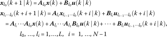
Consider the same RMPC problem in Section 7.1.1. At each time, an optimization problem (7.6) should be solved, with respect to the model (7.1) with polytopic uncertainties (7.2) and (7.3) and input and output constraints (7.4) and (7.5). According to the dual‐mode control, at time k, the future control inputs are assumed to be

(7.29)

where N is the length of the control horizon, which is the same as the optimization horizon. With this strategy, N free control inputs are firstly adopted to steer the system state into the terminal set and F is the gain of the state feedback control law in the terminal set.

Consider the min‐max performance index in the optimization problem (7.6) at time k:

Since two different control modes are adopted, J_∞(k) can accordingly be divided into two parts: the input and state items before and after the state entering the terminal set, respectively, i.e.

Firstly we derive the upper bounds of the maximum of the above two objective functions under polytopic uncertainty, respectively.

For the first part, using the system model (7.1) starting from x(k ∣ k) = x(k), it is easy to get the system states controlled by the N free control inputs as shown in (7.29):

or in the matrix form

(7.30)

where

(7.31)

Note that all the coefficients of matrices , in (7.30) are composed of A(k + i), B(k + i), which belong to the convex hull Π described by (7.2) and (7.3). If the combination parameters λ_l(k + i), l = 1, … , L, are time‐varying, the system uncertainty will be expanded with time. We use time‐related subscripts to distinguish time‐varying combination parameters and denote the combination parameters at time k + i as , l = 1, … , L, i = 0, 1, …, l_i = 1, … , L. Then .

To illustrate how the system uncertainty expands with time, start from the fixed x(k) at time k. For x(k + 1 ∣ k), uncertainty is only caused by [A(k) B(k)] and can be described by the polytope with L vertices , l₀ = 1, … , L. For x(k + 2 ∣ k), with the same procedure for each possible x(k + 1 ∣ k), uncertainty will be expanded due to [A(k + 1) B(k + 1)], which can be described by the same type of polytope with L vertices , l₁ = 1, … , L, but with independent combination parameters. Therefore the uncertainty of x(k + 2 ∣ k) should be described by a composite polytope with L² vertices , l₀ = 1, … , L, l₁ = 1, … , L. For example, the term A(k + 1)A(k)x(k) in x(k + 2 ∣ k) can be expressed by

With the above understanding, a convex hull with vertices can now be used to describe the polytopic uncertainties of corresponding to x(k + 1 ∣ k) to x(k + N − 1 ∣ k), i.e.

(7.32)

(7.33)

where is the vertex of the polytope . Similarly, a convex hull with vertices can be used to describe the polytopic uncertainties of corresponding to the terminal state x(k + N ∣ k):

(7.34)

(7.35)

Now we can define an upper bound for J₁(k). According to (7.30), it follows that

where , are the diagonal matrices, respectively, composed of , with proper dimensions. Remove the fixed term and define an upper bound γ₁ for the remaining part. It follows that

Due to the polytopic characters of the system parameters (7.32) and (7.33), it can be ensured by

(7.36)

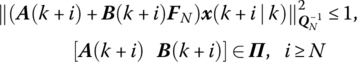
The input and output constriants (7.4) and (7.5) can be expressed by

where L_{u, i + 1}(L_{x, i}) is a proper matrix that selects u(k + i ∣ k)(x(k + i ∣ k)) from U(k)(X(k)) in (7.31). These two conditions can be ensured if the following LMIs are satisfied:

(7.37)

(7.38)

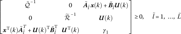
For the second part, the optimization problem with performance index J₂(k) is almost the same as that discussed in Section 7.1.1, with the only difference being that the initial state x(k ∣ k) is replaced by x(k + N ∣ k). We can similarly define a quadratic function V(x) = x^TPx to obtain an upper bound γ for the maximization problem, and define a controlled invariant set Ω = {x ∈ Rⁿ ∣ x^TQ⁻¹x ≤ 1} with a corresponding feedback control law u = Fx for all k + i, i ≥ N. Ω is just the terminal set that the system state should be steered to by the first N free control actions. Let P = γQ⁻¹ and F = YQ⁻¹; the following conditions similar to (7.12) and (7.14) to (7.16) can be obtained:

(7.39)

(7.40)

(7.41)

(7.42)

Then the min‐max problem (7.6) to be solved at time k can be converted into the following optimization problem:

(7.43)

Pluymer et al. thus proposed a control policy based on a tree structure spanned by free control inputs according to the character of polytopic uncertainty [7]. With this structure and the system model (7.1) to (7.3), the system state at any future time is uncertain but can be directly described by a polytope with corresponding state vertices (see Figure 7.1), where at each time a node means that a possible state vertex is driven by a corresponding input. In this way, the uncertainty expansion of system inputs and states could be explicitly described in accordance with the model uncertainty.

In Figure 7.1, at time k, the system state x(k) is known. According to the polytopic uncertainty of system model (7.1) to (7.3), the state under the control of u(k ∣ k) can be given by

which indicates that the system state x(k + 1 ∣ k) must be the convex combination of L state vertices , l₀ = 1, … , L (the nodes at time k + 1 in Figure 7.1), each corresponding to the fixed model with the vertex parameter , respectively.

For the sake of simplification, in the following we use the symbol l₀, … , l_m = * to represent l₀ =  * , ⋯, l_m = *, and to represent . For the system state x(k + 2 ∣ k), in terms of L state vertices , define different inputs for each state vertex and let

Similarly, under the control of , each state vertex will evolve to L state vertices , l₀, l₁ = 1, … , L. We have

where the system state x(k + 2 ∣ k) must be the convex combination of L² state vertices , l₁, l₀ = 1, … , L (i.e. the nodes at time k + 2 in Figure 7.1), where each corresponds to the fixed model with parameters of the vertex , respectively.

This procedure is continued until time k + N. As the result, the uncertainty of the system state x(k + i ∣ k) can still be described by polytope but the number of state vertices expands with time, as shown by the tree in Figure 7.1. Note that here a control policy of using different control inputs corresponding to each expanded state vertex is adopted, so the control inputs and the states in (7.31) are given by

(7.44)

where

(7.45)

Each time the control input is not a single one but is represented in a more detailed form corresponding to the tree structure

(7.46)

Then the state evolution (7.30) under the new control input U(k) with 1 + L + ⋯ + L^N − 1 components and new matrices with proper dimensions can be similarly derived. According to the new form of U(k) and new matrices, the optimization problem with constraint conditions similar to (7.43) and (7.36) to (7.42) can be established.

For the new formulated optimization problem, assume that it has an optimal solution U^*(k) at time k. Let l_i(k) be the subscript l_i defined at time k. Due to vertices expansion in Figure 7.1, has L^i − 1 components while has Lⁱ components . Obviously, for U(k) with this new structure, during proof of recursive feasibility, the candidate solution U(k + 1) at time k + 1 cannot be constructed by using a shifting operation to set as usual. However, as shown in Figure 7.1, u(k + 1 ∣ k + 1) corresponds to L with different l₀(k), and each corresponds to L resulting from with different l₀(k). Therefore each component in , i.e. , can be set by the weighted sum of , i.e.

(7.47a)

Similarly, set

(7.47b)

Since all are fixed at time k, the components of given by (7.47) are also fixed and the constructed U(k + 1) is available. Furthermore, with this setting and (7.44), it is easy to prove that

This indicates that the use of U(k) with new components in (7.46), on the one hand, makes the constructed U(k + 1) available at time k + 1 and, on the other hand, implies that the control inputs u(k + i ∣ k + 1) have the above relationship with u^*(k + i ∣ k) and x^*(k + N ∣ k), which is just what we originally expect to guarantee on the feasibility of the optimization problem (7.43) at time k + 1. For more details, refer to [8].

The design in this section uses the dual‐mode control concept. With additional free control inputs this kind of RMPC can improve the control performance and enlarge the initial feasible region, but at the cost of bringing a heavy online computational burden and difficuty on recursive feasibility, particularly when the combination parameters describing uncertainty are time varying.

7.1.4 Synthesis of RMPC with Multistep Control Sets

The RMPC described in the last section improves the control performance through adding free control inputs before employing a fixed‐state feedback control law, which brings more degrees of freedom for control but also increases the complexity to guarantee the recursive feasibility because of uncertainty expansion. This contradiction was resolved by introducing an open‐loop tree structure for state and control expansion. From another perspective, note that the state feedback law is often helpful to ensure recursive feasibility, such as its use in the terminal set. Li and Xi [9] proposed the concept of the multistep control set and used it to design a sequence of feedback control laws instead of free control inputs used in the dual‐mode framework. It seems an efficient way to guarantee recursive feasibility and thus is helpful to RMPC synthesis. In this section, we will briefly introduce the synthesis method of RMPC using multistep control sets.

(1) Multistep control set

From the definition, it is easy to see that any controlled invariant set is a one‐step control set. Furthermore, it is also easy to prove that a set is an s‐step control set if all the system states in it can be steered into an (s − 1)‐step control set by an admissible feedback control law. With this property, in the following we discuss how to design an s‐step ellipsoidal control set for the constrained polytopic uncertain system (7.1) to (7.5).

An s‐step control set can be designed by a series of ellipsoidal sets , i = 0, ⋯, s − 1. When the system state x is in the ellipsoidal set S_i − 1, one can use an admissible feedback control law F_i − 1x to steer the system state x into the ellipsoidal set S_i, while the last ellipsoidal set is a controlled invariant set with the feedback control law F_s − 1x in usual sense. Let . Conditions for S₀ as an s‐step control set can be given by

(7.48)

with

(7.49)

where conditions (7.48) ensure that the states in S_i − 1 enter into set S_i at the next time instant under the feedback control law u = F_i − 1x and meanwhile the set S_s − 1 is a controlled invariant set with the control law u = F_s − 1x. In addition, conditions (7.49) are used to ensure the input and state constraints, which are similar to (7.15), (7.16) in Section 7.1.1.

According to Definition 7.1 and the conditions (7.48) and (7.49), it is easy to show the following properties of a multistep control set.

(2) RMPC synthesis with a multistep control set

Now for the constrained uncertain system (7.1) to (7.5), consider the online optimization problem (7.6) at time k. Since the current system state x(k) is determined, its quadratic term can be firstly removed from J(k). Then rewrite the performance index in the optimization problem (7.6) as

Using the concept of a multistep control set, the following control strategy is adopted:

(7.50)

which implies that a series of ellipsoidal sets , i = 1, …, N is available to construct a multistep control set. At first, use a free control action u(k) to steer the system state x(k) into the ellipsoidal set S₁. Then for i = 1, …, N − 1, step by step use the feedback control law F_ix to steer the system state from the ellipsoidal set S_i to S_i + 1. The last ellipsoidal set S_N is a controlled invariant set where the feedback control law F_Nx is adopted. The control strategy π is to mix the quasi‐min‐max RMPC in [10] and the multistep control set, where the multistep control set is used as the terminal set of the quasi‐min‐max RMPC.

With control strategy π, choose quadratic functions V(i, k) = x^T(k + i ∣ k)P_ix(k + i ∣ k), i = 1, …, N − 1 for feedback control laws with gain F_i. Let P_i = P_N when i ≥ N. Similar to that in Section 7.1.1, the optimization problem to be solved at time k is derived as follows.

1. Imposing V(i, k) descending and satisfying the following conditions:
   (7.51)
2. Obtaining the upper bound of the objective function. Summing Eq. (7.51) from i = 1 to i = ∞, it follows that
   (7.52)

   Define the upper bounds for both and V(1, k):

   (7.53)
   (7.54)

   Then it follows that

   
3. Using u(k ∣ k) to steer the state x(k) into the ellipsoidal set :
   (7.55)
   (7.56)
   (7.57)
4. Steering the system state into the invariant set S_N by the N‐step control set:
   (7.58)
   (7.59)
   (7.60)
   (7.61)

   Now all of the above conditions will be converted into LMI forms. Let , , i = 1, …, N. Then the bound condition (7.54) is equivalent to the ellipsoidal set condition (7.55), and the multistep control set conditions (7.58) and (7.59) could be covered by the condition (7.51) together with (7.55). Therefore we only need to derive LMIs for other conditions. Similar to (7.14) but with a different P_i, the V(i, k) descending condition (7.51) can be written as

   (7.62)
   (7.63)

   The bound condition (7.53) will be

   (7.64)

   The condition (7.55) of x(k) steered into the ellipsoidal set S₁ can be written as

   (7.65)

   The input/output constraints at the first step (7.56) and (7.57) can be guaranteed by

   (7.66)
   (7.67)

   Referring to (6.13) and (6.15), the input/output constraints when x enters the multistep control set, i.e. (7.60) and (7.61), can be guaranteed by

   (7.68)
   (7.69)

   Now the RMPC algorithm based on the multistep control set can be given.

(3) Algorithm and robust stability

The following theorem is given for the stability of the above algorithm.

7.2.1 Synthesis with Disturbance Invariant Sets

Consider the following linear time‐invariant system with external disturbance

(7.71)

where A ∈ R^n × n, B ∈ R^n × m, and ω(k) ∈ Rⁿ represent the external disturbance. For the controlled system, the state and input constraints are given in general forms as

(7.72)

(7.73)

where Ω_x and Ω_u are the admissible sets of states and inputs, respectively. The notations of Minkowski set operations are also given as follows, which will be used later. For two sets A, B, set addition A ⊕ B ≜ {a + b ∣ a ∈ A, b ∈ B}, and set subtraction A ⊖ B ≜ {a ∣ a ⊕ B ⊆ A}.

If the disturbance is unbounded and varies arbitrarily, it is impossible to guarantee the constraints satisfied. In practical applications, the disturbance with a too large amplitude is often handled by some other measures. It is therefore generally assumed that the disturbance in (7.71) is bounded as

(7.74)

For system (7.71) to (7.74), the appearance of the disturbance makes the constraint handling much more complicated. If the approaches for RMPC synthesis in Section 7.1 are adopted, the influence caused by disturbance will be time varying, so the conditions that ensure the satisfaction of the input and state constraints are also time varying. In order to simplify the disturbance handling, Mayne et al. [11] proposed an approach to synthesize RMPC by using disturbance invariant sets. In the following, the main idea of this approach is introduced.

(1) Disturbance invariant set

Firstly, similar to the definition of the invariant set given in Chapter 6, the following definition on the disturbance invariant set is given.

It is obvious that if the system x(k + 1) = Ax(k) is unstable, no disturbance invariant set exists. For a control system given by x(k + 1) = Ax(k) + Bu(k) + ω(k), a feedback control law u(k) = Kx(k), often taken as the optimal controller of the unconstrained LQ problem with , can be used to make x(k + 1) = A_Kx(k) with A_K = A + BK stable. The disturbance invariant set Z designed for the resultant system x(k + 1) = A_Kx(k) + ω(k) makes x(k + 1) ∈ Z for all ω(k) ∈ Ω when x(k) ∈ Z and u(k) = Kx(k).

(2) RMPC synthesis by dividing the uncertain system into nominal and disturbed subsystems

Like the invariant set, the disturbance invariant set can keep the system state in it always within it by using the corresponding feedback control law even when the system is disturbed. This is convenient when handling constraints. Since system (7.71) is linear and of an additive character, [11] proposed an RMPC synthesis approach by dividing the system (7.71) into two subsystems:

(7.75a)

(7.75b)

(7.75c)

where subsystem (7.75a) is the nominal system of the original system (7.71). The basic idea to synthesize RMPC is as follows. Firstly, as mentioned above, use the feedback control law for the subsystem (7.75b) to get and find a disturbance invariant set Z for it. That is, under the control of , the state component will be kept in Z when the subsystem is disturbed by ω(k) ∈ Ω, i.e. A_KZ ⊕ Ω ⊆ Z. Then, for the nominal system (7.75a), use the conventional predictive control approach and optimize the nominal control component in order to steer the nominal state to the origin under tighter constraints, which take the influence of the disturbance into account. The real control input will be composed of . With this basic idea, when designing an RMPC using the disturbance invariant set, the admissible input set can be simply divided into two parts: one for designing the disturbance invariant set while the other for stabilizing the nominal system. After the disturbance has been separated, the nominal system will be stabilized by usual predictive control synthesis methods, which simplifies the design.

Synthesis of the disturbed subsystem

For subsystem (7.75b), a disturbance invariant set Z would be found such that with the feedback control law , if . The disturbance invariant set Z should be as small as possible to reduce conservativeness. Its form should also be suitable for optimization in the RMPC design. It has been suggested [11] that an algorithm be used to compute a polytopic, disturbance invariant, outer approximation of the minimal disturbance set, which can be taken as the disturbance invariant set Z here. If the nominal state reaches zero, the system state will always be in set Z. Therefore the disturbance invariant set Z serves as the “origin” for the original system with a bounded but unknown disturbance.

Synthesis of the nominal subsystem

Now turn to control of the nominal subsystem (7.75a). It is a linear time‐invariant system without uncertainty and disturbance, and thus can be easily handled by conventional predictive control approaches as presented in Chapter 6. The dual‐mode control strategy with N free control actions followed by the feedback control law is adopted. At time k, the cost function of the online optimization problem is given by

(7.76)

where the last term in (7.76) is the terminal cost function. This optimization problem is very similar to Problem PC4, (6.31) in Section 6.2.3, and could be solved in the same way. However, some important issues different from conventional predictive control should be pointed out.

1. Tighter state and input constraints. Since the optimization is only for the nominal subsystem (7.75a) with state and control input , the constraints (7.72) and (7.73) for the real system state x(k) and input u(k) cannot be directly used here. According to (7.75c), the admissible set Ω_x is shared by and . Therefore the admissible set of should be constructed by subtracting the admissible set of from Ω_x. A similar consideration is also for constructing the admissible set of as well as for setting the constraint on the terminal set X_f used in dual‐mode control. Therefore, we have tighter state, input, and terminal constraints as follows:
   (7.77)
   (7.78)
   (7.79)
2. Initial state as an optimization variable. When solving the optimization problem at time k, the real system state x(k) is assumed available and is used as the initial state of the optimization in conventional predictive control. However, the optimization here is with respect to and . Nothing is known about and thus cannot be set as the initial state in the optimization, but would be taken as an additional optimization variable and handled as a parameter of the control law. It can vary but would be constrained by the following initial condition with the known system state x(k):
   (7.80)

   Thus, the optimization problem at time k can be formulated as

   (7.81)

   where . the terminal set X_f and the weighting matrix P in the terminal cost function should satisfy the following conditions:

   (7.82a)
   (7.82b)

   where the first condition is to ensure that the terminal set X_f is a controlled invariant set for the nominal system (7.75a) with state component and feedback control law 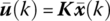when enters X_f, while the second condition is to ensure that the value of the objective function is nonincreasing within the terminal set; see condition A4 in (6.38).

   Note that the disturbance invariant set Z, the terminal set X_f, and set operations can be calculated off‐line. Thus the online optimization problem (7.81) is simple and straightforward.

   After the optimal and U^*(k) are solved, the following control law will be applied to the real system:

   (7.83)

   The associated optimal state sequence as well as the optimal value of the cost function can also be obtained.

(3) Theoretical properties of the RMPC controller

For the optimization problem (7.81), the optimal solution and the control law depend on the system state x(k). The following important results were given in [11] after investigating the theoretical properties of the solution and the controlled system:

1. For all x(k) ∈ Z, J^*(x) = 0, , U^*(x) = {0, … , 0}, X^*(x) = {0, … , 0}, and the control law .
2. Let X_N be the set of x(k) for which there always exists satisfying (7.77) to (7.80). Suppose that x(k) ∈ X_N so that (, U^*(k)) exists and is feasible for Problem (7.81) at time k. Then, for all , (, ) with is feasible at time k + 1 and .
3. The set Z is robustly exponentially stable for the uncertain controlled system , ω(k) ∈ Ω with a region of attraction X_N, which means there exists a c > 0 and a γ ∈ (0, 1) such that for the initial state x(0) ∈ X_N and admissible disturbance sequence ω(k) ∈ Ω, k ≥ 0, any solution x(k) of above system satisfies d(x(k), Z) ≤ cγ^kd(x(0), Z) for all k ≥ 0, i.e. the real system state x(k) will exponentially approach the disturbance invariant set Z, where d(x, Z) is the minimal distance of a point x from the set Z.

The RMPC approach presented above makes use of the linear and additive character of the original system to divide it into two subsystems. A modified optimization problem for the nominal subsystem is solved online where the initial nominal state is taken as an additional optimization variable. A suitable Lyapunov function is accordingly selected that has value zero in the set Z, with which the robust exponential stability of Z can be proved. It is shown that the real state of the controlled system is always along a tunnel with the nominal system state as the center and the disturbance invariant set Z as the cross‐section. This idea led to the tube technique, which was later widely used in RMPC synthesis for systems with uncertainty and disturbance.

7.2.2 Synthesis with Mixed H₂/H Performances

In this section, we introduce another kind of RMPC for systems with disturbance, which adopts H₂ and H_∞ performance in optimization. Consider the following disturbed system:

(7.84)

where x(k) ∈ Rⁿ, u(k) ∈ R^m, and z(k) ∈ R^r are system state, control input, and controlled output, respectively. A(k) ∈ R^n × n, B(k) ∈ R^n × m, and [A(k) B(k)] ∈ Π with

(7.85)

The disturbance ω(k) ∈ R^s is bounded as

(7.86)

where and q > 0 are known.

The constraints on the system inputs and maesurable states are given by

(7.87)

(7.88)

where Ψ_j is the jth row of the state constraint matrix Ψ ∈ R^s × n. Note that (7.87) is just the peak bound constraint on the input components, as discussed in Section 6.1.4, while (7.88) is the bound constraint on the linear combination of the states.

Unlike system (7.71) discussed in the last section, system (7.84) includes not only the external disturbance but also the model uncertainty. Although the disturbance invariant set can also be designed for the system with model uncertainty, the resultant design may be conservative.

It is well known that the LQ performance index corresponds to an H₂ optimal control problem, which is generally useful for optimal controller design and has traditionally been adopted as the objective function in RMPC to achieve a better control performance, while the H_∞ performance index is known as a useful criterion on a control system for its ability to reject disturbance. In order to achieve both the desired disturbance rejection and a good dynamic performance, it is a natural idea to combine these two performances, i.e. using a mixed H₂/H_∞ performance, to synthesize RMPC. This idea actually came from research of robust control and was later adopted in RMPC study. In this section we briefly introduce this kind of RMPC synthesis approach presented in [12].

For system (7.84) to (7.88), consider the following two performance requirements:

1. H_∞ performance requirement: under the zero‐initial condition, the controlled output z(k) satisfies
   (7.89)
2. H₂ performance requirement: the controlled output z(k) satisfies
   (7.90)

To optimize both performance indices, it is usual to firstly assign an upper bound on one performance index and then design RMPC by online optimizing the other performance index with the above upper bound condition as an additional constraint. Here the H₂ performance index α is taken as the online optimization objective of RMPC and the H_∞ performance index γ > 0 is set as a fixed scalar to deal with (7.89) as a constraint.

Following the above idea, choose the RMPC control law as u(k) = Fx(k). At time k, based on the initial state x(k), an optimization problem with the performance indices (7.89) and (7.90), rewritten with the initial time k, can be solved online. Define the quadratic function . Denote ϕ(k) = A(k) + B(k)F and ϕ_l = A_l + B_lF, l = 1, … , L. We can get

(7.91)

where

Note that from (7.86) the disturbance is energy‐bounded. This means that, if the closed‐loop system is stable, then . Thus, summing (7.91) from k to ∞ can yield

It follows that

(7.92)

From (7.92), it can be seen that:

1. When x(k) = 0, the H_∞ performance requirement (7.89), i.e.
   

   can be ensured if M(k + i) ≤ 0.

2. When M(k + i) ≤ 0, the H₂ performance requirement (7.90) can be guaranteed if the following condition holds:
   (7.93)

   where M(k + i) ≤ 0 can be rewritten as

   (7.94)

   which can be reformulated as the LMIs

   

   Let Q = αP⁻¹, F = YQ⁻¹. Note that ϕ(k + i) is a convex combination of ϕ_l. Left‐ and right‐multiply the above inequality by diag (α^1/2P⁻¹, α^1/2I, α^1/2I, α^1/2I, α^1/2I). Then the following condition can be obtained which can ensure the above inequality:

   (7.95)

   Meanwhile, (7.93) can be rewritten into LMI as

   (7.96)

   which implies that , and thus the current system state x(k) belongs to an ellipsoidal set Ω = {x ∣ x^TQ⁻¹x ≤ 1}. Therefore, as (6.14) in Section 6.1.4, the input constraints (7.87) can be written as

   (7.97)

   The state constraints (7.88) can be written as

   (7.98)

   However, due to the existence of disturbance, the condition M(k + i) ≤ 0, i.e. (7.95), is not enough to ensure V(x(k + 1)) − V(x(k)) ≤ 0 in (7.91), and Ω = {x ∣ x^TQ⁻¹x ≤ 1} is not a controlled invariant set, i.e. the system state x(k + 1) cannot be ensured to be in Ω even when the current state x(k) ∈ Ω. This also leads to a problem with recursive feasibility and will be solved by adding some new conditions as follows.

   For the current state x(k) ∈ Ω, it follows that x(k + 1) = ϕ(k)x(k) + B_ωω(k). To ensure the state x(k + 1) ∈ Ω, divide it into two parts: the nominal substate and the substate v(k) = B_ωω(k) affected by disturbance. The condition of x(k + 1) in the set Ω = {x ∣ x^TQ⁻¹x ≤ 1} can then be represented by

   

   Let 0 < b < 1 be a parameter chosen in advance. The above matrix inequality can be ensured if both of the following two conditions hold:

   (7.99)
   (7.100)

   where (7.100) indicates that ω(k) should be in an ellipsoidal set . According to (7.86), all the disturbances ω(k) ∈ Π_q ≔ {ω ∣ ω^Tq⁻¹ω ≤ 1}. Therefore (7.100) can be ensured if , which can be rewritten as

   (7.101)

   Meanwhile, (7.99) means , where Q_b = (1 − b)(Q − Q_ω). Since x(k) ∈ Ω = {x ∣ x^TQ⁻¹x ≤ 1}, this can be ensured if

   (7.102)

   Let . Referring to (7.91), we get

   (7.103)

   where M_b(k + i) ≤ 0 can be ensured by

   (7.104)

   Note that is the nominal substate with ω(k) = 0; from (7.103) it is known that (7.104) can guarantee (7.102) and then (7.99). It is also tighter than condition (7.95) due to Q_b < Q and thus can cover (7.95). With conditions (7.101) and (7.104), the recursive feasibility, i.e. state x(k + 1) ∈ Ω if x(k) ∈ Ω, can be ensured even if a disturbance exists, and the decreasing of V(x(k)) can be guaranteed.

   As mentioned above, here the H_∞ performance γ is used as a constraint and the H₂ performance α would be optimized. By fixing γ and choosing the parameter b in advance, the online optimization problem of RMPC can be formulated as follows:

   (7.105)

   In the above, the basic idea of the RMPC synthesis with mixed H₂/H_∞ performance is introduced. It adopts the control startegy with the unique feedback control law, which may be conservative. New design approaches were also developed to improve the performance, which can be found in the literature.

7.3.1 Difficulties for Robust Predictive Controller Synthesis

The RMPC synthesis approach presented in Section 7.1.1 can also be applied to systems with structural uncertainties. In [1], a kind of system with structural feedback uncertainty is converted into an uncertain LTV system and RMPC for it is synthesized in the same way but with different LMI forms. The basic idea of synthesizing RMPC and the specific technique of handling constraints in [1] have an important impact on subsequent researches of robust predictive control, which have been shown, for example, in the other parts of Section 7.1. However, the approach presented in [1] still has some limitations:

1. To make the design simple, a unique feedback control law is adopted in [1], which strictly restricts the structure of the future control sequence. As the result, the control performance could not be further improved because of the lack of more degrees of freedom for control.
2. In practical applications, the feasible region of the predictive controller, i.e. the region of system initial states with guaranteed stability, is preferred to be as large as possible such that the closed‐loop stability can be guaranteed for a larger region of system states. However, with the unique feedback control law as in Section 7.1.1, the closed‐loop system is robustly stable only when x(0) ∈ Ω, i.e. the feasible region is obviously restricted by Ω.
3. The optimization problem in [1] should be solved online according to the rolling style of predictive control. The problem scale increases rapidly with the system dimension and the number of vertices of the uncertain model, which will lead to a heavy computational burden and make it difficult to be implemented in real time. Furthermore, the optimization problem with the LMI formulation cannot be solved as efficiently as that with the QP formulation.

In fact, the above limitations reflect the main difficulty in RMPC synthesis, i.e. the contradiction among the requirements on feasible region (reflecting the region of the system states with guaranteed stability), online computational burden (reflecting whether the algorithm can be applied in real time), and control performance (reflecting the optimization effect of the designed predictive controller). In order to illustrate this, consider the general method adopted in the stable and robust predictive controller synthesis shown in Figure 7.2.

At each step of rolling optimization, take the following predictive control strategy: start from the initial system state, adopt N free control inputs in the optimization horizon to steer the system state into the terminal constraint set, and then use the fixed feedback control law in the terminal constraint set to drive the system state to zero.

According to Section 6.2.3, the terminal set constraint is a relaxation of the zero terminal constraint and is easier to implement than it. However, the zero terminal constraint means that the system state will remain at the origin when it arrives at the terminal, while the terminal set constraint means that the system state is not zero when it enters the terminal set and a fixed state feedback control law is still needed to steer the state asymptotically to the origin. In this sense, the performance of the control system corresponding to the terminal set constraint is in general inferior to that of the zero terminal constraint. The larger the terminal set, the worse the control performance will be. From the point of view of improving the control performance, a smaller terminal set is often preferable.

The feasible region of the predictive controller characterizes the applicable region of the system states starting from which the stability or robust stability of the closed‐loop system can be theoretically guaranteed. In practice, the initial state outside the feasible region may also lead to stable results, but without a theoretical guarantee. From the point of view of the applicable range of the designed predictive controller, a larger feasible region is often preferable.

With the general control strategy mentioned above, N free control inputs before entering the terminal set and the feedback control law after entering the terminal set need to be solved online. The larger the optimization horizon N, the heavier the online computational burden will be. To reduce the online computational burden, a smaller N is more acceptable.

However, the above three requirements are often contradictory in a specific synthesis algorithm of predictive control. Referring to Figure 7.2, for example,

• A larger feasible region can be achieved by enlarging the terminal set or increasing the optimization horizon, but the control performance will be degenerated or the computational burden will be increased, respectively.
• Reducing the terminal set may improve the control performance, but will reduce the feasible region. If at the same time keeping the feasible region unchanged, the optimization horizon must be increased and thus the computational burden will be increased.
• Decreasing the optimization horizon can reduce the online computational burden, but the feasible region will be reduced if the terminal set is unchanged to maintain the control performance. If the feasible region must be maintained, the terminal set has to be enlarged and the control performance will be sacrificed.

The above‐mentioned contradiction between control performance, feasible region, and online computational burden is the critical issue faced by predictive control synthesis, especially in the synthesis of robust predictive controllers. Some typical approaches to improve the design in [1] have been introduced in Section 7.1. In the following, we further introduce some other approaches that also show the variety of the RMPC research.

7.3.2 Efficient Robust Predictive Controller

In order to enlarge the feasible region and reduce the online computational burden, Kouvaritakis et al. proposed an RMPC algorithm named efficient robust predictive control (ERPC) [13]. The basic idea of ERPC is as follows. Firstly, an off‐line design using a fixed feedback control law is proposed that satisfies the input constraints and can robustly stabilize the controlled system. Then, additional degrees of freedom for control are introduced and an invariant set for the augmented system is solved off‐line, which has the maximum projection set in the original state space. When online, the additional variables are optimized in order to achieve a better control performance.

For the system (7.1) to (7.3) with polytopic uncertainties, consider the input constraints

(7.106)

where u_j(k) is the jth component of control input u(k) ∈ R^m. The RMPC for this system is formulated as solving an infinite horizon optimization problem at each time k with the cost function

(7.107)

Due to the polytopic uncertainty of the model, the optimization for (7.107) is indeed a “min‐max” problem as in (7.6). In the following, the main idea of ERPC is briefly introduced.

(1) Design the feedback control law and handle the input constraints

Firstly, a fixed feedback control law u(k) = Kx(k) is designed that stabilizes all the models of system (7.1) to (7.3) without considering the input constraints (7.106). Define the controlled invariant set of system (7.1) to (7.3) with this feedback control law as

(7.108)

Let Φ(k) = A(k) + B(k)K; then we have . Due to the polytopic property of the model uncertainty, it follows that

(7.109)

where Φ_l = A_l + B_lK, l = 1, …, L. With the control law u(k) = Kx(k), the input constraints (7.106) can be written as

where is the jth row of K. If the system state x(k) belongs to the invariant set Ω_x, it follows that

Thus the input constraints can be satisfied if

(7.110)

Then, based on (7.109) and (7.110), adopt the method in Section 7.1.1 to design RMPC and obtain K, Q_x, such that system (7.1) to (7.3) can be robustly stabilized and the input constraints (7.106) are satisfied. This is simply the RMPC strategy presented in [1].

(2) Introduce perturbations to form the augmented system

In order to enlarge the feasible region and improve the control performance, it was suggested in [13] that extra degrees of freedom should be introduced by using perturbations c(k + i) on the fixed state feedback law. The control law was then modified as

(7.111)

where c(k + i) = 0, i ≥ n_c. This means that c(k + i), i = 0, …, n_c − 1 as additional input variables can be used to increase the degree of freedom for RMPC synthesis. Then the closed‐loop system can be expressed by

By introducing the augmented state,

(7.112)

it can be formulated as an autonomous system

(7.113)

where

For the autonomous system (7.113), get the controlled invariant set like (7.108):

(7.114)

where Q_z satisfies

(7.115)

Meanwhile, note that the control law is now (7.111), i.e.

Referring to (7.110), the input constraints (7.106) can be ensured if

(7.116)

where is the jth row of the identity matrix with dimension m.

(3) Design the invariant set to enlarge the feasible region

Now consider the influence of introducing additional input variables to the invariant set of augmented system, which is also the feasible region of the RMPC. The matrix in (7.114) can be divided into four blocks corresponding to x and f: , , , and , where . Then, from (7.114) it follows that

(7.117)

Therefore, if we let , then for all , the above inequality is degenerated to the condition in (7.108). However, if f ≠ 0, from (7.117), it is possible to make the projection set of Ω_z on x space larger than Ω_x by properly choosing f. For example, if we let , the projection of Ω_z on x space can be given by

Since , if , it follows that Ω_x ⊆ Ω_xz. That is, the invariant set on x space can be enlarged by the additional input variables. Figure 7.3 shows the enlarged invariant set in the x space after the state space has been augmented.

In order to achieve a general formulation, denote the projection set of the invariant set Ω_z, i.e. (7.114) on x space as

(7.118)

Let x = Tz with T = [I  0] of dimension n × (n + mn_c) and make a transformation for the LMIs implied in (7.114):

Thus it is known that Q_xz = TQ_zT^T in (7.118). If is expressed by four blocks defined as above, we can calculate exactly. Therefore, a larger feasible region than Ω_x can be achieved by making use of the additional input variables to design Ω_z such that Q_xz ≥ Q_x.

(4) Implementation and algorithm

Then, according to the above analysis, the ERPC synthesis can be summarized as:

1. Design the optimal feedback control law u(k) = Kx(k) for the unconstrained system (7.1) to (7.3) by using the usual robust control method with a specific optimization requirement, such as minimizing a worst‐case cost or optimizing a nominal performance.
2. Introduce f and construct the augmented autonomous system (7.113) with K and design the invariant set Ω_z of the autonomous system such that its projection set Ω_xz on x space is as large as possible and Q_z satisfies the invariant set condition (7.115) as well as the input constraint condition (7.116).
3. The current augmented state z(k) belongs to set Ω_z, i.e. condition (7.114) holds.
4. The degree of freedom of f is used to optimize the system performance.

Note that (1) and (2) are independent from the system state x(k) and thus can be solved offline to reduce the online computational burden. Therefore the control algorithm can be divided into two parts: offline and online.

It was proved in [13] that if K, Q_z, and n_c exist such that x(0) ∈ Ω_xz, ERPC with Algorithm 7.3 will robustly stabilize system (7.1) to (7.3) with satisfaction of the input constraints. Kouvaritakis et al. also pointed out in [14] that the optimization problem (7.120) can be efficiently solved by well‐known techniques, such as the Newton–Raphson (NR) method. Compared with the conventional RMPC method in [1], the control performance can be improved and the feasible region is enlarged by using the extra degrees of freedom introduced by f, while the online computational burden is greatly reduced because the main part of the computation has been moved to off‐line. Thus, ERPC makes a good trade‐off among the control performance, feasible region, and online computational burden.

7.3.3 Off‐Line Design and Online Synthesis

The EPRC presented in the last section greatly reduces the online computational burden by an off‐line design, which shows the possibility to make a trade‐off among the control performance, feasible region, and online computational burden by combining off‐line and online computations. In view of the heavy online computational burden of the RMPC synthesis approach in [1], Wan and Kothare [15] proposed an offline design/online synthesis method for an RMPC design based on the ellipsoidal invariant set.

Consider the RMPC synthesis problem in Section 7.1.1. For the uncertain system (7.1) to (7.3) with input and state constraints (7.4) and (7.5), given an initial state x, if it is feasible for Problem (7.17), then we can solve Problem (7.17) to get the optimal solution γ, Q, Y, with which an ellipsoidal invariant set Ω = {x ∈ Rⁿ ∣ x^TQ⁻¹x ≤ 1} and its corresponding feedback control law u(k) = Fx(k) with F = YQ⁻¹ can be obtained. Since all the system states in the set Ω can be steered to the origin by the feedback control law, the design of an ellipsoidal invariant set is independent from the current system state x(k). Thus, the core idea of [15] is to use off‐line to construct a series of ellipsoidal invariant sets and calculate their corresponding feedback control laws and online to determine the most suitable ellipsoidal invariant set and the corresponding feedback control law in terms of an actual system state and then to calculate the required control action. This can be described by the following algorithm in detail.

Using Algorithm 7.4, the online computational burden can be greatly reduced. However, from the online Algorithm 7.1 it is known that the optimal control law and the corresponding invariant set depend on the system state. While in Algorithm 7.4, with a limited number of preserved invariant sets, the same state feedback control law may be used for different states that belong to the same region between two adjacent invariant sets. This means that such a control law is not necessarily the optimal one and the control performance might be degenerated. It is obvious that increasing the number of presented invariant sets may achieve a better control performance. However, due to the limitation of storage as well as the off‐line computational burden, the number of chosen initial feasible states is restricted. In the following, two ways to further improve the control performance for Algorithm 7.4 are briefly introduced.

In [15], an additional constraint is imposed on the invariant set obtained by the off‐line part of Algorithm 7.4 as follows:

(7.121)

If the sets in the look‐up table can satisfy conditions (7.121), then the online part of Algorithm 7.4 can be modified as follows.

Robust stability of the closed‐loop system controlled by Algorithm 7.4 or its modified version was proved in [15]. In both cases, the obtained feedback control law between sets Ω_i and Ω_i+1 is guaranteed to keep x(k) within Ω_i and converge it into Ω_i+1 (see [15] for details). Since the feedback control law is online adjusted according to the current system state, a better control performance can be achieved.

Another way to improve Algorithm 7.1 that is different from the method in [15] is based on the fact that the convex combination of multiple ellipsoidal invariant sets is also an invariant set. For n ellipsoidal invariant sets , h = 1, …, n with Q_h, Y_h, γ_h satisfying (7.14) to (7.16), their convex combination is also an ellipsoidal invariant set with , , satisfying (7.14) to (7.16), where λ_h ≥ 0, h = 1, …, n, . This can be easily shown by multiplying a parameter λ_h to the inequalities in (7.14) to (7.16):

and then sum them for h = 1, …, n. Note that the condition (7.14) also implies V(i, k) descending and satisfying (7.7) and is tighter than needed by the invariant set.

Since conditions (7.14) to (7.16) are independent from the real‐time system state x(k), it is possible to off‐line design a series of invariant sets with different performance indices like that in Algorithm 7.4 and then to online optimize the convex combination coefficients to achieve a better control performance. The off‐line design is often formulated as several optimization problems under constraints (7.14) to (7.16), each with a specific performance index such as maximizing the covered region of the ellipsoidal invariant set S_h with a fixed γ_h or pursuing a better control performance by setting a much smaller γ_h [9]. With respect to Algorithm 7.1, the online synthesis should take the constraint (7.12) into account with off‐line solved Q_h, Y_h, γ_h, h = 1, …, n, and the real‐time state x(k), formulated as follows.

With the above modified version 2, although an optimization problem with LMI formulation still needs to be solved online, the number of online optimization variables and the rows of LMIs decrease greatly because the optimization variables are just the combination coefficients. Therefore, with this algorithm the online computational burden can be greatly reduced. The basic idea of using the convex combination of multiple invariant sets as an invariant set and the synthesis approach of off‐line designing multiple invariant sets and online optimizing the combination coefficients can also be applied to other similar cases such as the multistep control sets presented in Section 7.1.4.

7.3.4 Synthesis of the Robust Predictive Controller by QP

In the above sections, LMI is clearly a main tool used to formulate the online optimization problem for RMPC synthesis. This means that the semi‐definite programming (SDP) solver should be adopted online, which may lead to a heavy online computational burden. Furthermore, when dealing with asymmetrical constraints, there is often a need to reformulate them into symmetrical ones such that LMIs can be derived through ellipsoidal invariant sets, which obviously makes the result conservative. To overcome these shortcomings, it was also suggested to formulate the RMPC as a QP problem with which a good trade‐off among feasible region, control performance, and online computational burden could be achieved. In the following, we briefly introduce the synthesis method used by Li and Xi [16].

Consider the uncertain system (7.1) to (7.3). In order to simplify the presentation, the considered constraints are given in a very general form:

(7.123)

where and are the column vectors with appropriate dimensions and the number of constraints is p.

Consider the objective function of RMPC with an infinite horizon as

(7.124)

where . To guarantee the closed‐loop stability, the control strategy is chosen as

(7.125)

where K is a feedback gain and c(k + i) is the additional control input. The control strategy in (7.125) is the same as (7.111) in ERPC (see Section 7.3.2). However, in order to enlarge the feasible region, here a dual‐mode control strategy is adopted, i.e. to use free control inputs to steer the system state to a terminal invariant set Ω_f in N steps and then in Ω_f to use the feedback control law u = Kx to stabilize the system. Using a similar method to that in Section 7.1.1, a terminal cost function can be used as an upper bound to replace the sum of infinite terms after N steps in the cost function. Thus, the online optimization problem can be formulated as

(7.126)

where the feedback control gain K and the weighting matrix of the terminal cost function P_f should satisfy the following conditions:

(7.127)

which implies that V(i, k) = x(k + i ∣ k)^TP_f  x(k + i ∣ k) is imposed to descend and to satisfy conditions (7.7) for all possible [A(k + i) B(k + i)] ∈ Π and J(k) after i = N has an upper bound similar to (7.8), .

The terminal invariant set Ω_f and its corresponding feedback control gain K are necessary for RMPC synthesis. They can be calculated off‐line by the following algorithm.

After P_f, Ω_f, K are solved off‐line by using Algorithm 7.5, the online optimization problem (7.126) can be formulated as an QP problem, where the constraints of future control inputs should be linear and the objective function should be quadratic.

(1) Linear constraints

The constraints in the optimization problem (7.126) are all linear if the terminal set Ω_f is selected as a polyhedral one. All these constraints are with respect to the future system states and control inputs. Due to the polytopic uncertainty of the system parameters, if the control strategy (7.125) is adopted, similar to the discussion in Section 7.1.3, the future system state trajectory will belong to a convex hull, whose vertices are the state trajectories along with the vertex trajectory of polytopic models (see (7.45)). For example, at time k + 1,

where Φ_l = A_l + B_lK and ζ_i(k) = [x^T(k), c^T(k), … , c^T(k + i)]^T. Similarly,

(7.129)

Due to the polytopic property of the system uncertainty, it is obvious that the future states x(k + i + 1 ∣ k) in the state/input constraints and the terminal set constraint in (7.126) can be replaced by all corresponding state vertices . These constraints can be rewritten as

(7.130)

(7.131)

where

(2) Quadratic cost function

Since the optimization problem (7.126) is a min‐max problem, the upper bound of J(k) is used as the objective function when converting it to a QP problem. In [16] it has been shown that if a vector w ∈ Co{w_i, i = 1, … , L}, then , where Q > 0. From time k to k + N, the future state trajectory belongs to a convex hull and thus the objective function J(k) of the predicted state trajectory must satisfy J(k) ≤ max {J_i(k)}, where and P_i can be calculated according to the vertex sequences of different future state trajectories. Therefore, to get the upper bound of J(k), the following optimization problem should be solved to obtain the matrix P:

(7.132)

where P_i is determined by the quadratic terms in J(k) and corresponding , l₀, … , l_i = 1, …, L, i = 1, …, N − 1. If P has been solved, can be used as the quadratic cost function for the minimization problem in (7.126).

(3) QP formulation

With the off‐line solved feedback gain K, terminal set Ω_f, terminal weighting matrix P_f, and matrix P in the upper bound of the cost function, the optimization problem (7.126) can be formulated as the following QP problem:

(7.133)

From the above analysis it can be seen that since the constraints are commonly linear, the critical issue to transfer the RMPC optimization problem to a QP problem is to adopt the polyhedral invariant set as the terminal set and to design a quadratic function as the upper bound of the objective function.

The condition that ensures the closed‐loop system robustly stable is also given in [16], where a Lyapunov function is adopted and the recursive feasibility is easily proved using the feasible solution at time k + 1 constructed by shifting forward the last N − 1 terms in and setting its last term as zero.

For the QP problem (7.133), in addition to the usual QP solving methods such as the active set method, the multiparameter programming method is also helpful in reducing the online computational burden. Note that the optimization problem (7.133) is given with respect to the optimization variables c(k + i) and the current system state x(k), i.e. it has the form

Therein, the state x(k) is time‐varying and determines the constraints. According to Bemporad et al. [18], the current system state x(k) can be handled as parameters and the explicit solution c(k) = F_ix(k) + g_i can be obtained for the parameter x(k) within the ith subset. Thus, by the multiparameter programing method, the x space is divided into several subsets and then the corresponding explicit solutions can be obtained and stored off‐line. When online, instead of solving the QP problem, it is only required to search the subset to which the state x(k) belongs and then to look up the corresponding feedback gain (F_i, g_i) to construct the current control input.

References

- 1 Kothare, M.V., Balakrishnan, V., and Morari, M. (1996). Robust constrained model predictive control using linear matrix inequalities. Automatica 32 (10): 1361–1379.
- 2 Cuzzola, F.A., Geromel, J.C., and Morari, M. (2002). An improved approach for constrained robust model predictive control. Automatica 38 (7): 1183–1189.
- 3 Mao, W.J. (2003). Robust stabilization of uncertain time‐varying discrete systems and comments on “an improved approach for constrained robust model predictive control”. Automatica 39 (6): 1109–1112.
- 4 Michalska, H. and Mayne, D.Q. (1993). Robust receding horizon control of constrained nonlinear systems. IEEE Transactions on Automatic Control 38 (11): 1623–1633.
- 5 Wan, Z. and Kothare, M.V. (2003). Efficient robust constrained model predictive control with a time varying terminal constraint set. Systems and Control Letters 48: 375–383.
- 6 Ding, B., Xi, Y., and Li, S. (2004). A synthesis approach of on‐line constrained robust model predictive control. Automatica 40 (1): 163–167.
- 7 Pluymers, B., Suykens, J.A.K., and De Moor, B. (2005). Min–max feedback MPC using a time‐varying terminal constraint set and comments on “Efficient robust constrained model predictive control with a time‐varying terminal constraint set”. Systems and Control Letters 54: 1143–1148.
- 8 Ding, B.C. (2010). Modern Predictive Control. Boca Raton: CRC Press.
- 9 Li, D. and Xi, Y. (2009). Design of robust model predictive control based on multi‐step control set. Acta Automatica Sinica 35 (4): 433–437.
- 10 Lu, Y. and Arkun, Y. (2000). Quasi‐min‐max MPC algorithms for LPV systems. Automatica 36 (4): 527–540.
- 11 Mayne, D.Q., Seron, M.M., and Raković, S.V. (2005). Robust model predictive control of constrained linear systems with bounded disturbances. Automatica 41 (2): 219–224.
- 12 Huang, H., Li, D., and Xi, Y. (2012). Design and ISpS analysis of the mixed H2/H∞ feedback robust model predictive control. IET Control Theory and Applications 6 (4): 498–505.
- 13 Kouvaritakis, B., Rossiter, J.A., and Schuurmans, J. (2000). Efficient robust predictive control. IEEE Transactions on Automatic Control 45 (8): 1545–1549.
- 14 Kouvaritakis, B., Cannon, M., and Rossiter, J.A. (2002). Who needs QP for linear MPC anyway? Automatica 38 (5): 879–884.
- 15 Wan, Z. and Kothare, M.V. (2003). An efficient off‐line formulation of robust model predictive control using linear matrix inequalities. Automatica 39 (5): 837–846.
- 16 Li, D. and Xi, Y. (2011). The synthesis of robust model predictive control with QP formulation. International Journal of Modeling, Identification and Control 13 (1–2): 1–8.
- 17 Pluymers, B., Rossiter, J.A., Suykens, J.A.K., and Moor, B.D. The efficient computation of polyhedral invariant sets for linear systems with polytopic uncertainty, Proceedings of 2005 American Control Conference, Portland, OR (8–10 June 2005), 804–809.
- 18 Bemporad, A., Morari, M., Dua, V., and Pistikopoulos, E.N. (2002). The explicit linear quadratic regulator for constrained systems. Automatica 38 (1): 3–20.