
4
Quantitative Analysis of SISO Unconstrained Predictive Control Systems
In Chapter 3, some trend conclusions on the stability of the DMC controller and on closed‐loop robust stability affected by the DMC filter were given by transforming the DMC algorithm into the IMC structure and analyzing the corresponding characteristic polynomials. Here “trend” means that in the theorem conditions some design parameters are set as extreme values, such as M = 1, P → ∞, r → ∞, α sufficiently small, etc. (see Theorems 3.1 to 3.3 and 3.6, respectively), which is sometimes also called the “limiting case” or “marginal stability” in the literature and is caused by the lack of an explicit relationship between the design parameters and the characteristic polynomial.
Indeed, since the appearance of predictive control algorithms such as DMC and GPC, in order to get more guidance for applications, many efforts have been put into exploring the relationship between the design parameters and the control performance. Except for the trend conclusions mentioned above, more explicit and analytical relationships between design parameters and system performance were required. During the 1980s and a little later, some interesting quantitative results for analyzing GPC and DMC algorithms were achieved. Since these studies focused on quantitative analysis for existing predictive control algorithms, we call the theoretical study for this purpose quantitative analysis theory of predictive control.
In this chapter, we will introduce some important results of quantitative analysis theory of predictive control. Firstly, theoretical analysis of the GPC algorithm given by Clarke and Mohtadi [1] is briefly introduced, which is based on the Kleinman controller in the time domain. The main part of this chapter is devoted to the Z domain analysis of predictive control systems. With the help of the IMC structure, the minimal form of the DMC controller is derived and proved to be identical to the GPC controller in the IMC structure. Through exploration of the intrinsic relationship between the control parameters and the coefficients of the characteristic polynomial, the coefficient mapping of open‐loop and closed‐loop characteristic polynomials is established, based on which the quantitative relationship between the design parameters and the closed‐loop performance can be analyzed. The derived results hold for both DMC and the GPC algorithm and cover the result derived by theoretical analysis in the time domain.
Quantitative analysis needs analytical expressions of the controlled system, which is impossible for constrained predictive control algorithms because the control law should be obtained by solving an optimization problem and could not be expressed in a closed form in general. Even in the unconstrained case, for multivariable predictive control systems, the analytical expression of the control law in state space or the controller in the IMC structure is difficult to derive and would be very complex. Therefore, the quantitative analysis in this chapter is mainly for SISO unconstrained predictive control systems. Furthermore, the study will focus on investigating the quantitative influence of the design parameters on stability and dynamic behavior of the closed‐loop system in the nominal case, i.e. without model mismatch and disturbance. Therefore the model and the plant will be uniformly represented by the same state equation or transfer function.
4.1 Time Domain Analysis Based on the Kleinman Controller
Some stability conditions were given for the GPC system in [1] in 1989. In order to utilize the mature theoretical results in optimal control theory, Clarke and Mohtadi firstly transformed the GPC control law into an LQ (Linear Quadratic) control law in state space. Their main contribution is that they deduced the stability condition of the GPC closed‐loop system through investigating under which condition the GPC control law can be equivalently transformed into the Kleinman controller, a specific class of controllers with guaranteed stability in the LQ control theory. This method is novel and the result directly describes a quantitative relationship between the design parameters and the closed‐loop stability. In this section, referring to [1, 2], we briefly introduce the critical issues of this work with some expansions.
(1) The LQ control law of GPC
As described in Section 2.2, in the GPC algorithm, when the stochastic disturbance ξ(t) is removed, the system model (2.19) is equivalent to the transfer relationship (2.20b) between u and y. The transfer function between Δu and y can accordingly be obtained as follows:

where an ≠ 0, ![]() . Note that this transfer function is of the order of max (n + 1, nb + 1). To simplify the symbols, assume that n ≥ nb. Also assume that the numerator polynomial and the denominator polynomial are coprime. Then the above system can be transformed into a realization in the state space,
. Note that this transfer function is of the order of max (n + 1, nb + 1). To simplify the symbols, assume that n ≥ nb. Also assume that the numerator polynomial and the denominator polynomial are coprime. Then the above system can be transformed into a realization in the state space,

where x(k) ∈ Rn + 1, A, b, cT are related to the coefficients of the transfer function but are not unique. Note that (cT A b) is both controllable and observable.
With respect to the performance index of GPC (2.24), consider the deterministic case and not lose generality; let w = 0. Denote

Then the GPC performance index (2.24) can be rewritten as

This is a standard LQ control problem. According to the standard solution of LQ control, the control law can be obtained as
where P(k + 1) can be solved by the following Riccati iterative formula

Here (4.4) is the control law when GPC is described as an LQ problem, called the LQ control law of GPC. This transformation is significant because there already exist quite good results on the control law and stability of the LQ control problem, which can be utilized to investigate the stability of the GPC control law. For the sake of simplification, in the following we use Pi to represent P(k + i).
(2) The Kleinman controller with stability
Early in 1974, Kleinman proposed a specific controller as he investigated the LQ control problem. For an n‐dimensional state space model with m inputs
he gave the following result.
(3) The explicit expression of P1 in the control law (4.4)
From (4.2) it is known that Qi and λi in the Riccati iterative formula are not constant and depend on the optimization horizon and the control horizon. If we assume that N1 = NU, according to the values of Qi and λi in different ranges, the iterative formula (4.5) can be written as

Based on (4.8), start from ![]() and iterate from i = N2 − 1 to i = N1; it follows that
and iterate from i = N2 − 1 to i = N1; it follows that

![]() can be also represented by
can be also represented by

Since (cT A) is observable, if N2 − N1 + 1 ≥ n + 1, then the rank of ![]() is n + 1, i.e.
is n + 1, i.e. ![]() is invertible.
is invertible.
Then start from ![]() and continue to iterate from i = N1 − 1 to i = 1. According to the iterative formula (4.8), at i = N1 − 1 we have
and continue to iterate from i = N1 − 1 to i = 1. According to the iterative formula (4.8), at i = N1 − 1 we have
Since ![]() is invertible, using the matrix inversion formula
is invertible, using the matrix inversion formula
the above formula can be rewritten as

If A is invertible, from above it is known that ![]() is also invertible and
is also invertible and
Then the following can be similarly deduced:
and furthermore

When λ → 0+, this can be approximately written by

where (4.9) actually gives the expression of P1 (i.e. P(k + 1)).
(4) The control law (4.4) in the form of the Kleinman controller (4.7)
The control law (4.4) can be rewritten as
where
Using the matrix inversion formula it follows that

Using (4.9), this can be written as

Obviously it has the same form as the Kleinman controller (4.7).
(5) Deadbeat and stability conditions for GPC
In the last two steps, the assumed condition N1 = NU leads to the iterative formula (4.8), and the assumed condition N2 − N1 + 1 ≥ n + 1 guarantees that ![]() is invertible and deduces the expression of (4.9) when λ → 0+. With these conditions, the GPC control law (4.4) can be equivalent to the Kleinman controller with feedback gain (4.11). Since the system (4.1) is n + 1 dimensional, from Lemma 4.1 it is known that the system (4.1) is closed‐loop stable with the GPC control law if N1 − 1 ≥ n + 1.
is invertible and deduces the expression of (4.9) when λ → 0+. With these conditions, the GPC control law (4.4) can be equivalent to the Kleinman controller with feedback gain (4.11). Since the system (4.1) is n + 1 dimensional, from Lemma 4.1 it is known that the system (4.1) is closed‐loop stable with the GPC control law if N1 − 1 ≥ n + 1.
In addition to making the GPC control law (4.4) equivalent to the Kleinman controller, Clarke and Mohtadi also discussed the following special case.
(6) Extension of the results
Since the condition of Theorem 4.1 is very demanding (such as asking the matrix A to be invertible) and the range of the design parameters involved is quite limited, there were some subsequent works along this line in the 1990s. For various possible cases of denominator and numerator polynomial orders n and nb in the GPC model (2.19), Ding and Xi [2] extended the Kleinman controller for possible singular A and gave the closed‐loop stability or deadbeat conditions for it. They also discussed the equivalence of the LQ control law of GPC and the extended Kleinman controller for sufficiently small λ and obtained the following conclusions.
4.2 Coefficient Mapping of Predictive Control Systems
In this section, the coefficient mapping of the characteristic polynomials between the plant and the controlled predictive control system will be deduced based on the IMC structure in the Z domain, which is the basis of quantitatively analyzing the predictive control systems in the next section. Under the IMC framework, the expression of the GPC controller is firstly given, the minimal form of the DMC controller is revealed, and the uniformity of both controllers is proved. Then the coefficient mapping of the characteristic polynomials between the plant and the controlled system is established, based on which stability and dynamic performance can be investigated uniformly for both DMC and GPC control systems.
4.2.1 Controller of GPC in the IMC Structure
Similar to deducing the IMC structure of the DMC algorithm in Section 3.2, the expressions of all the components of the GPC algorithm in the IMC structure can also be deduced (see [4]). Since the focus of this chapter is on analyzing the closed‐loop performance without model mismatch and disturbance, according to (3.2), only the expression of the GPC controller in the IMC structure needs to be deduced. In order to facilitate a comparison with the DMC algorithm, the model online identification and adaption is not considered here. Assume n = nb + 1 in the model (2.19), and rewrite the coefficients of B(q−1) as
Then the plant transfer function can be written as

The GPC control law (2.30) is given by
where

The reference trajectory w in (4.18) is given by (2.32) as
where c is the reference input

and according to (2.27) the vector f can be written as

where

Substitute (4.19) and (4.20) into (4.18), and note that y(z)/u(z) = z−1B(z)/A(z); the Z transfer function of the GPC controller (the transfer function from reference input c to control action u) can then be given by

It is clear that the vectors F and H appearing in the transfer function of the GPC controller GC(z) are related to Ej and Fj, and need to be calculated recursively. In order to analyze the system performance, in the following Ej and Fj will be eliminated such that the resultant expression of the controller is only related to the plant parameter A, {gi}, and the control parameter di. Firstly, the following Lemma is given.
In order to compare this with the DMC controller, in the following, the reference trajectory will not be considered, i.e. α = 0 and d0 = 0. The GPC controller (4.24) then has the form

4.2.2 Minimal Form of the DMC Controller and Uniform Coefficient Mapping
The GPC controller (4.26) in the IMC structure deduced in the last section clearly explains the compensation mechanism of GPC for system dynamics, while the DMC controller (3.10) in the IMC structure shows nontrivial characters because it adopts a nonminimum model with step response coefficients. For example, the order of the model depends on the model length N with great arbitrariness and the control result is insensitive to the model order. The transfer function of such a model has all the zeros at the origin, which makes it difficult to explain the compensation mechanism of DMC for system dynamics. However, although different models are adopted by DMC and GPC, in principle the same control result should be achieved if the rolling optimization strategy of GPC (2.24) is coincident with that of DMC (2.3) and the additional reference trajectory in the GPC algorithm is out of consideration. In this section, the relationship of the DMC controller (3.10) and the GPC controller (4.26) is explored.
Assume that the minimum model of a stable plant with the step response {ai} is given by

For simplicity it is assumed that pn ≠ 0, mn ≠ 0, i.e. the model order is n. For the same plant, it is obvious that the model (3.9) is an approximation of the above model under the assumption that ai ≈ aN, i ≥ N. Note that there exists the same relationship between the model parameters mi and pi and the step response parameters ai as given by Lemma 4.3; only the symbols ai, bi, and gi in (4.22) should be replaced by pi, mi, and ai here.

Figure 4.1 The compensation property of the DMC controller: (a) in the form of a nonminimal controller, (b) in the form of a minimal controller [6].
Source: Reproduced with permission from Taylor and Francis and Copyright clearance center.
4.3 Z Domain Analysis Based on Coefficient Mapping
According to Theorem 4.4, it is now possible to uniformly analyze the system performance of the two main predictive control algorithms, DMC and GPC. As mentioned above, we will focus on the stability analysis without model mismatch and disturbance. In this case, the closed‐loop predictive control system can be uniformly described by (4.28), and the closed‐loop stability will be uniformly analyzed by using the coefficient mapping (4.30) between the open‐loop and the closed‐loop characteristic polynomials. In this section, quantitative analysis for the DMC algorithm will be given based on coefficient mapping in the Z domain. In the meantime, corresponding conclusions for the GPC algorithm are also given in parallel.
4.3.1 Zero Coefficient Condition and the Deadbeat Property of Predictive Control Systems
The DMC closed‐loop system for the nth‐order plant (4.27) can be described by (4.28). It is known from the coefficient mapping relationship (4.30) that the closed‐loop system is of order n + 1, and the coefficients of the characteristic polynomial are given by

where p = [1 p1 ⋯ pn]T. Firstly, consider how to select the design parameters to make some ![]() . Note that when deducing the minimal form of the DMC controller in Section 4.2.2, Lemma 4.3, i.e. (4.22), is utilized to obtain
. Note that when deducing the minimal form of the DMC controller in Section 4.2.2, Lemma 4.3, i.e. (4.22), is utilized to obtain

for i = n + 2, … , N + n − 1, while each pi* in (4.30), i = 1, … , n + 1, cannot be eliminated to zero in the same way because both 0 and 1 appear in the corresponding expression (4.31). In order to solve the problem, the following lemma is given, showing an important relationship between the parameters in the DMC algorithm.
By combining (3) in the Corollary 4.2 and the Lemma 4.6, the following theorem is given.
4.3.2 Reduced Order Property and Stability of Predictive Control Systems
Combining Lemma 4.5 and Lemma 4.6, the relationship between the closed‐loop order and the design parameters can be further derived.

Figure 4.2 Simulation results of the system in Example 4.2 with different parameters.

Figure 4.3 The relationship of the GPC closed‐loop order and N1, NU [7].
The above theorems characterize the performances of the DMC closed‐loop system more deeply than that given in Section 3.2.1. They are suitable for general plants and the parameter selection is not limited to extreme cases, giving not only the stability result of the closed‐loop system but also a quantitative description of closed‐loop dynamics. This indicates that the coefficient mapping of the characteristic polynomials plays an important role in the closed‐loop analysis of predictive control systems.
It should be pointed out that in order to highlight the main idea and simplify formula deduction, it is assumed that the denominator polynomial and the numerator polynomial in the plant model (4.27) have the same order n. For the more general case with possible different orders, similar results can be achieved by using the same method and details can be referred to [7].
4.4 Quantitative Analysis of Predictive Control for Some Typical Systems
The coefficient mapping relationship (4.30) is also useful to the predictive control design for some typical systems, such as the first‐order inertia process and the second‐order oscillation system. In this section, based on coefficient mapping, predictive control for these systems is quantitatively analyzed in more detail, which provides the basis for the analytical design of predictive control systems.
4.4.1 Quantitative Analysis for First‐Order Systems
A large number of industrial processes can be approximately described by the following typical plant – a first‐order inertia process with time delay
where K is the plant gain, τ is the time delay, and T is the time constant of the first‐order inertia process. All these parameters are easy to identify by directly using its step response. To simplify the discussion it is assumed that K = 1. After sampling with period T0 and holding, the Z transfer function of this typical plant can be given by
where σ = exp(−T0/T), l = τ/T0 is a nonnegative integer. For the case that τ is not an integer multiple of T0, the method presented here can also be used to deduce corresponding results and thus it is not discussed here.
The typical plant (4.36) has a delay time of l steps. According to Section 3.2.3, if model mismatch is not considered, select the optimization horizon as P + l and the error weighting matrix as block diag[0l × l, QP × P]; then its DMC design can be attributed to the design for the following delay‐free first‐order plant with the performance index (2.3):
The closed‐loop response of plant (4.36) under DMC control coincides with that of plant (4.37), except that an additional l steps delay time will appear in the output. Therefore, in the following, it is only required to discuss the DMC parameter selection for the first‐order inertia plant (4.37).
The coefficients of the unit step response of the first‐order inertia plant (4.37) are given by
which satisfy

In order to investigate the quantitative relationship between the design parameters and the system performances, firstly consider the case of the control horizon M ≥ 2. Using Theorem 4.5 to the first‐order inertia plant (4.37), the following theorem can be obtained.
Table 4.1 The correlations and characters of σ, λ, and β.
| Symbols | Correlation with | Ranges and characters | ||
| Modeling | Control strategy | |||
| T0/T | P | r | ||
| σ | √ | × | × | decreases with increasing T0/T, |
| λ | √ | √ | × | decreases with increasing P, |
| β | √ | √ | √ | decreases with increasing r, |
Now a detailed analysis of the properties of the closed‐loop system is given as follows.
(1) Closed‐loop characteristic polynomial and stability
According to (4.29), (4.30), and (4.37), the DMC controller can be written as

where

With the above parameter setting, it follows that

and

Then we have the following theorem.
(2) Dynamic performance of the closed‐loop system
In the case without a model mismatch, it is known from (3.2) that the Z transfer function of the closed‐loop system is given by
The following two cases are discussed:
1) The case where r = 0. In this case β = 1, ![]() , and
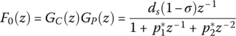
, and ![]() . Note that ds = β(1 − σ + λ)/(1 − σ), the Z transfer function of the closed‐loop system is given by
. Note that ds = β(1 − σ + λ)/(1 − σ), the Z transfer function of the closed‐loop system is given by

This indicates that when r = 0 the closed‐loop system is still a first‐order inertia component, with the steady‐state gain 1 and the time constant
The controlled system has a faster response than the original one because T* < T. Furthermore, T* increases with P because σ − λ increases with P. Particularly for P = 1, λ = σ, T* → 0+, the system output reaches the steady‐state value only after a one‐step delay. For sufficiently large P, λ → 0, T* → T, close to the original response of the plant.
Note that σ − λ in (4.41) can also be explicitly expressed by P and σ:

where σ is only related to the sampling period T0 and the plant time constant T. Scaled with T, the relationship between T* with the sampling period T0 and the optimization horizon P is given in Figure 4.4. It is shown that T* increases monotonically both with P and T0. Particularly for small T0 or small P, T* changes almost linearly with T0.
2) The case where r > 0. In this case the closed‐loop Z transfer function is given by

This is a second‐order component with steady‐state gain of 1. Denote

The roots of Δ = 0 are given by

It is easy to show that β2 > β1 > 0 and

Due to the correspondence between β and r, denote ri = (1 − βi)s2/βi, i = 1, 2; then

Given σ and P, β1 and β2 can be calculated according to (4.44), and then r1 and r2 are easy to obtain. In the range r1 > r > r2, Δ < 0, the closed‐loop system (4.43) has two conjugate complex poles and is stable but with oscillation. If r ≥ r1 or r ≤ r2, Δ ≥ 0, the closed‐loop system (4.43) has two real poles, corresponding to two first‐order inertia dynamics, and the time constant will depend on that of the dominant one
The above quantitative analysis for the first‐order system is summarized in Table 4.2.

Figure 4.4 The relationship between the closed‐loop time constant T* and P, T0.
Table 4.2 Performance analysis of DMC for typical first‐order systems.

4.4.2 Quantitative Analysis for Second‐Order Systems
In this section, we briefly give some results on the quantitative analysis of predictive control for typical oscillation systems. Consider the typical second‐order oscillation plant with natural frequency ω0 and damping coefficient ξ(<1) described by the following transfer function:

This system has a damped natural frequency ![]() , oscillatory period T = 2π/ωn, and its unit step response is given by
, oscillatory period T = 2π/ωn, and its unit step response is given by

where
Denote the sampling period as T0(T0 < π/2ωn), Ω = ωnT0, σ = exp(−ηT0) = exp(−Ωf2). It is obvious that cosΩ > 0, 0 < σ < 1, and the sampled values of the system step response can be given by
It is easy to prove the following lemma.
Define

We then have the following lemma.
- Dynamic performance of the closed‐loop system. Denote
 . Then (4.55) has a pair of conjugate complex roots if Δ < 0 and the closed‐loop system exhibits a second‐order oscillation response. In this case, the closed‐loop system can be fitted by a standard second‐order oscillation component whose corresponding parameters are marked by an asterisk, i.e.

Compared with (4.55), it follows that

Then the damped natural frequency and the damping coefficient can be given by
(4.56)
The closed‐loop response can be fitted using the step response
(4.57)
and the maximal overshoot can be obtained by
(4.58)
For a given second‐order oscillation plant (4.46) with known ω0 and ξ, the closed‐loop predictive control system may still be a second‐order oscillation one. Its characteristic parameters of the oscillation response (damped natural frequency, damping coefficient, maximal overshoot) can be directly estimated when the sampling period T0 and the design parameter P are given.
(2) Closed‐loop performance analysis with control weighting (r > 0)
With control weighting in the performance index (2.3), i.e. r > 0, the closed‐loop characteristic polynomial is given by
- Stability
Combined with (4.54), the necessary and sufficient conditions for the stable closed‐loop system are given by

where C1, C2 are referred to the proof of Theorem 4.10 and the parameters in (4) are given by

which are only related to the plant parameters, sampling period, and optimization horizon, and are independent of β or the control weighting r.
In Theorem 4.10 it has been proved that C1 > 0, C2 > 0; thus the conditions (1) to (3) obviously hold. The necessary and sufficient condition for the stability of the closed‐loop system can thus be summed up as to whether the condition (4) is established or not. Note that

where C3 are referred to the proof of Theorem 4.10. Since 0 < β ≤ 1, if A ≤ 0, then P(β) > 0 holds for all 0 < β ≤ 1, i.e. the closed‐loop system is stable for all r. If A > 0, there are two possible cases:
Case 1: B2 − 4AC < 0. In this case P(β) > 0 holds for all 0 < β ≤ 1, i.e. the closed‐loop system is stable for all r.
Case 2: B2 − 4AC ≥ 0. In this case P(β) has two real roots, denoted by β1, β2, and β1 ≤ β2. According to 0 < β ≤ 1 and P(β) > 0 for β = 0 or β = 1, we have the following possibilities for the positions of β1 and β2.
When 1 < β1 ≤ β2 or β1 ≤ β2 < 0, P(β) > 0 holds for all 0 < β ≤ 1 and the closed‐loop system is stable for all r.
When 0 < β1 ≤ β2 < 1, P(β) ≤ 0 holds for β1 ≤ β ≤ β2, and the closed‐loop system is unstable at the corresponding range of the design parameter r2 ≤ r ≤ r1.
Based on the above analysis, the following theorem can be obtained.
- Dynamic performance of the closed‐loop system. When r > 0, the closed‐loop system exhibits a third‐order dynamic response. According to the expression of p*(z) in (4.59), it is known that for sufficiently small r (i.e. β → 1), the dynamic response is close to the second‐order process. With the increase of r, another characteristic motion is markedly enhanced. When r → + ∞ (i.e. β → 0), the (1) in stability condition (4.60) tends to zero, indicating that the system has a real root close to z = 1, corresponding to the main characteristic motion of the system. From the simulation results for r varying in Figure 4.8, the correctness of the above analysis can be verified.
The main results of the above quantitative analysis for second‐order oscillation systems are summarized in the following Table 4.3.

Figure 4.5 Relationship between ξ* (solid line),  (dotted line), and P, T0.

Figure 4.6 Comparison of the actual (above) and fitted (below) response (P = 4). (a) T0 = 0.04 s; (b) T0 = 0.16 s; (c) T0 = 0.25 s .

Figure 4.7 The stable region of r in relationship with T0, P for Example 4.4.

Figure 4.8 Closed‐loop response with r for Example 4.4 (T0 = 0.04, P = 2).
Table 4.3 Performance analysis of DMC for typical second‐order oscillation systems.

4.5 Summary
In this chapter, for predictive control algorithms such as GPC and DMC, the quantitative relationships between the design parameters and the closed‐loop performances are explored both in the time domain and in the Z domain. In the time domain, the GPC control law is firstly transformed into the LQ control law in the state space. By studying under which conditions the GPC control law is equivalent to the stable Kleinman controller, stability/deadbeat conditions of the closed‐loop GPC system are derived in relation to the design parameters. In the Z domain, using the IMC structure, the expression of the GPC controller and the minimal form of the DMC controller are derived and both are proved identical. The coefficient mapping between the open‐loop and closed‐loop characteristic polynomials is then established. Based on the coefficient mapping, deadbeat/stability conditions of the closed‐loop DMC or GPC system are derived in relation to the design parameters, and the quantitative relationship between the design parameters and the reduced‐order property of the closed‐loop system is also given.
By analyzing the performances of the GPC system based on the Kleinman controller in the state space, conclusions are obtained in relation to the system order, but are independent of specific parameters. The analysis based on coefficient mapping of the characteristic polynomials in the Z domain can not only give qualitative conclusions on whether the controlled system is stable/deadbeat but also the reduced‐order property of the closed‐loop system. The concrete expression of the closed‐loop dynamic response can be given when combining with specific parameters of the system, which provides more information for the closed‐loop performance analysis of predictive control systems.
The coefficient mapping is also adopted to quantitatively analyze the control performances of predictive control for some typical plants: the first‐order inertial plant and the second‐order oscillation plant. When setting partial design parameters, more concrete and explicit results on the stability and closed‐loop dynamic response can be derived that are only dependent on a few remaining design parameters. This may be helpful to predictive control design. Particularly, a great number of systems can be approximated by these two typical plants and only some key parameters of the plant should be known beforehand, which are very easy to identify using the step response or according to the process data.
References
- 1 Clarke, D.W. and Mohtadi, C. (1989). Properties of generalized predictive control. Automatica 25 (6): 859–873.
- 2 Ding, B. and Xi, Y. (2004). Stability analysis of generalized predictive control based on Kleinman’s controllers. Science in China, Series F 47 (4): 458–474.
- 3 Kleinman, D.L. (1974). Stabilizing a discrete, constant, linear system with application to iterative methods for solving the Riccatti equation. IEEE Transactions on Automatic Control 19 (3): 252–254.
- 4 Xi, Y. and Li, J. (1991). Closed‐loop analysis of the generalized predictive control systems. Control Theory and Applications 8 (4): 419–424 (in Chinese).
- 5 Xi, Y. and Zhang, J. (1997). Study on the closed‐loop properties of GPC. Science in China, Series E 40 (1): 54–63.
- 6 Xi, Y. (1989). Minimal form of a predictive controller based on the step response model. International Journal of Control 49 (1): 57–64.
- 7 Zhang, J. Study on some theoretical issues of predictive control. PhD thesis, 1997, Shanghai Jiao Tong University (in Chinese).