
8
Covariance‐Based Interpolation
The previous chapter has shown the importance of maintaining the image edges in image interpolation to obtain a natural‐looking interpolated image. We have discussed the basic structure and model of image edges. The multi‐resolution analysis presented in the chapter on wavelet (Chapter ) has shown that an ideal step edge obeys the geometric regularity property [43 ], which refers to the correlation structure of an ideal step edge being independent of the scale of the image. In other words, the correlation structure of the local region that has enclosed an edge feature in the low‐resolution image should have a similar correlation structure in the corresponding region in the high‐resolution image. The edge‐directed interpolated algorithms presented in the last chapter aim to preserve the correlation structures across scales by estimating the unknown pixels with the consideration of the locations and orientations of the image edges. The locations and the orientations of the image edges are specified by explicit edge map obtained through some kind of edge detection techniques. There are several problems associated with such approach. Firstly, the edge detection technique quantized the edge orientation in finite number of cases. As a result, the interpolation results can only preserve limited classes of correlation structures during the interpolation process. In other words, the geometric regularity cannot be fully preserved between the low‐resolution image and the interpolated high‐resolution image. Secondly, the edge detection algorithm has detection accuracy problems in both the spatial location of the edge pixel and the orientation of the associated edge. As a result, the edge‐directed interpolation algorithm might falsely preserve a nonexisting edge structure and results in image artifacts with unnatural appearance and low in peak signal‐to‐noise ratio (PSNR).
To achieve good image interpolation result, the geometric regularity property should be fully exploited. Various algorithms have been proposed in literature that aim to preserve the geometric regularity between the low‐resolution image and the interpolated high‐resolution image, which include directly considering the geometric regularity in spatial domain [12, 38 ], reformulating the problem into a set of partial differential equations [6, 47 ], and constructing a convex set of geometric regularity [54 ], and proposed a projection‐onto‐convex‐set algorithm to achieve an interpolated image with the best matched correlation structure between the low‐resolution image and the interpolated high‐resolution image.
Among all the algorithms in literature, the new edge‐directed interpolation (NEDI) [40 ] proposed by Li and Orchard in 2001 is regarded as the first edge‐adaptive interpolation method that can fully exploit the geometric regularity problem between the original image and the interpolated image. Instead of considering an explicit edge map obtained from some edge detection techniques, the NEDI performs linear prediction to estimate the unknown pixel intensity to interpolate low‐resolution image directly on the covariance of a local window across the low‐resolution image and the interpolated high‐resolution image. The covariance preservation between the low‐resolution image and the interpolated high‐resolution image is known as the preservation of “geometric duality,” which indirectly maintains the geometric regularity. The formulation and accuracy of the linear prediction involves the statistical model of a natural image and the minimization of the prediction error by considering the “minimum mean squares error” (MMSE). In this chapter, the second‐order statistical model of natural image and the basic of MMSE optimization‐based image interpolation method will be discussed.
8.1 Modeling of Image Features
Among various interpretation of natural image, one of the interpretations considers natural image as combination of patches of smooth regions and texture‐rich regions. Image structure within the same region should be homogeneous. A detailed discussion on how different regions in an image are classified has been presented in Chapter . It has been shown that the human visual system (HVS) is sensitive to the region boundaries, while the boundaries can be completely closed to enclose an object or formed by short segments with arbitrary length and open ends lying in arbitrary directions. These boundaries are known as the “edges.” Figure 8.1 shows portion of the pixel intensity map extracted from the Cat image, where abrupt pixel intensity changes are observed across the boundary and two relatively uniform regions are observed on the two sides of the edge. However, it is vivid that the distribution of the pixel intensity in each region has a certain pattern but the patterns in the two regions may not be consistent. Though there are intensity changes, the HVS is only sensitive to those with significant changes – in other words, more sensitive to the location where abrupt changes occur. To understand the importance on preserving edges in image interpolation, we can consider the geometric constraint in edge preservation for image interpolation through both psychological and information theoretical aspects. In the psychological point of view, HVS is sensitive to edge sharpness and artifacts appearing around edges instead of just the contrast of the homogeneous patches on the two sides of the edge. In the information theoretical aspect, estimating unknown pixel intensity along edge orientation will reduce the dimensionality of the estimation problem and render better estimation results. It has been shown in Section 2.5 that the edge property is the best analyzed by high‐order statistics. In the next section, we shall discuss the modeling and analysis of edge features in digital image through second‐order statistics. The presented statistical model will be applied in subsequent sections to develop image interpolation algorithms that preserve the geometric duality between low‐ and high‐resolution images.

Figure 8.1 3D visualization of image containing edge: (a) original image with a selected portion under illustration, (b) the zoom‐in 3D map, and (c) the intensity plot of the selected portion.
8.2 Interpolation by Autoregression
It has been discussed in Chapter that the interpolation problem can be formulated as a weighted sum problem between the neighboring pixels surrounding the pixel to be interpolated. The bilinear interpolation makes use of the four neighboring pixels, and bicubic interpolation makes use of the 16 neighboring pixels. Let us consider the example of interpolating the missing pixel ![]() shown in Figure 8.2 . When the image is modeled as random field, a fourth‐order linear predictive image interpolation problem can be formulated as
shown in Figure 8.2 . When the image is modeled as random field, a fourth‐order linear predictive image interpolation problem can be formulated as

which is also known as a fourth‐order autoregressive model with ![]() being the model parameters relating to the four neighbors of the interpolating pixel and
being the model parameters relating to the four neighbors of the interpolating pixel and ![]() is the prediction error term. In particular, for
is the prediction error term. In particular, for ![]() image interpolation,
image interpolation, ![]() . As a result, Eq. (8.1 ) can be rewritten as
. As a result, Eq. (8.1 ) can be rewritten as

which is an autoregressive model on ![]() to produce
to produce ![]() . In other words, Eq. (8.2 ) is a
. In other words, Eq. (8.2 ) is a ![]() image interpolation formulation with
image interpolation formulation with ![]() in Eq. (8.3 ) as a pixel in the interpolated image. Unlike the nonparametric image interpolation methods discussed in Chapters 4–6, which use the same
in Eq. (8.3 ) as a pixel in the interpolated image. Unlike the nonparametric image interpolation methods discussed in Chapters 4–6, which use the same ![]() all over the whole image (such as in the case of bilinear, bicubic, discrete cosine transform (DCT), etc. based image interpolation methods). It has been demonstrated in Chapter 7 that the model parameter
all over the whole image (such as in the case of bilinear, bicubic, discrete cosine transform (DCT), etc. based image interpolation methods). It has been demonstrated in Chapter 7 that the model parameter ![]() should adapt to the local image features, such that different
should adapt to the local image features, such that different ![]() should be applied to interpolate pixels within the image with different features. There are a vast number of research works presented in literature discussing what is the best model to adapt the modeling coefficients
should be applied to interpolate pixels within the image with different features. There are a vast number of research works presented in literature discussing what is the best model to adapt the modeling coefficients ![]() , including those presented in Chapter 7. In this section, we shall exploit the modeling coefficient
, including those presented in Chapter 7. In this section, we shall exploit the modeling coefficient ![]() that minimizes the prediction error squares given by
that minimizes the prediction error squares given by

where ![]() is the model coefficient vector and
is the model coefficient vector and ![]() is the vector of the four neighboring pixels surrounding
is the vector of the four neighboring pixels surrounding ![]() . The vector
. The vector ![]() is known as the pixel intensity vector of the prediction window, where the subscript (
is known as the pixel intensity vector of the prediction window, where the subscript (![]() ) indicates the location of the vector in the image. This vector shall bear the variable
) indicates the location of the vector in the image. This vector shall bear the variable xLR in the MATLAB implementation in later sections.

Figure 8.2 Coefficients of linear prediction.
Without loss of generality, we shall consider the noise‐free case, such that the image is a locally stationary Gaussian process and the optimal coefficient is given by

Solving for ![]() yields
yields

where ![]() and
and ![]() are the correlation matrix and vector of the high‐resolution image, respectively. It is however very sad to learn that the above solution to the problem of optimal prediction coefficients
are the correlation matrix and vector of the high‐resolution image, respectively. It is however very sad to learn that the above solution to the problem of optimal prediction coefficients ![]() will not be readily available, because of the nonavailability of both correlation matrix and vector. Some kinds of assumptions are required to create these matrix and vector to obtain the optimal predication coefficients. This is where the NEDI comes into the picture, because with a very simple assumption that fits right into most of the real‐world picture, these unavailable correlation matrix and vector will suddenly become available with the given low‐resolution image alone.
will not be readily available, because of the nonavailability of both correlation matrix and vector. Some kinds of assumptions are required to create these matrix and vector to obtain the optimal predication coefficients. This is where the NEDI comes into the picture, because with a very simple assumption that fits right into most of the real‐world picture, these unavailable correlation matrix and vector will suddenly become available with the given low‐resolution image alone.
8.3 New Edge‐Directed Interpolation (NEDI)
NEDI is developed to remedy the interpolation problem in Eq. (8.5 ), such that the missing information required to compute the optimal prediction coefficient ![]() will become available where the NEDI assumes the following image model assumptions:
will become available where the NEDI assumes the following image model assumptions:
- 1. Natural image is a locally stationary second‐order Gaussian process.
- 2. Low‐resolution and high‐resolution images have similar second‐order statistics in corresponding local patches.
As a result, the image is completely described by the second‐order statistics, and hence the interpolated pixels can be obtained from the linear prediction (autoregression) model in Eq. ( 8.2 ) with the optimal prediction coefficients given by Eq. ( 8.5 ). In particular, the second assumption provided a method to obtain the correlation matrix and vector for Eq. ( 8.5 ) to compute the optimal prediction coefficients, where the correlation matrix and vector in the high‐resolution image are the same as that obtained in a similar region of the low‐resolution image. This property is known as the geometric duality.
In layman's terms, the interpolation making use of geometric duality assumes that the covariance matrices of a small local window associated with pixels within a small region are homogeneous. As a result, the optimal interpolation weighting ![]() can be obtained as the average of the optimal interpolation weighting of its neighboring pixels:
can be obtained as the average of the optimal interpolation weighting of its neighboring pixels:

where ![]() are the optimal prediction coefficients of the pixel with index with respect to a particular pixel
are the optimal prediction coefficients of the pixel with index with respect to a particular pixel ![]() . The summation is performed over all the pixels within a small region surrounding
. The summation is performed over all the pixels within a small region surrounding ![]() , which we shall call the mean covariance window for the pixel
, which we shall call the mean covariance window for the pixel ![]() . All pixels in the mean covariance window and
. All pixels in the mean covariance window and ![]() are the local low‐resolution pixels. The mean covariance window has
are the local low‐resolution pixels. The mean covariance window has ![]() pixels that are associated with the low‐resolution image pixels and are neighbors of
pixels that are associated with the low‐resolution image pixels and are neighbors of ![]() . Note that the optimal interpolation for each low‐resolution pixel in the mean covariance window, which we denote them as
. Note that the optimal interpolation for each low‐resolution pixel in the mean covariance window, which we denote them as ![]() is given by Eq. ( 8.5
) as
is given by Eq. ( 8.5
) as
where the correlation matrix and vector are given by
Consider a fourth‐order autoregressive linear prediction problem. The ![]() is a
is a ![]() vector containing the four 8‐connected neighbors of
vector containing the four 8‐connected neighbors of ![]() . The optimal
. The optimal ![]() for the interpolation of pixel
for the interpolation of pixel ![]() is given by Eq. (8.6 ), which is the mean
is given by Eq. (8.6 ), which is the mean ![]() over all
over all ![]() mean covariance windows
mean covariance windows
where ![]() is a
is a ![]() matrix and
matrix and ![]() is a
is a ![]() vector. The MATLAB function in Listing 8.3.1 implements the above optimal
vector. The MATLAB function in Listing 8.3.1 implements the above optimal ![]() estimation with a given
estimation with a given ![]() (in MATLAB
(in MATLAB C), local window pixel intensity vector ![]() (in MATLAB
(in MATLAB win) within the mean covariance window (in MATLAB mwin), and a new parameter ![]() (in MATLAB
(in MATLAB t), which will be discussed in a sequel. It should be noted that the dimension of C in MATLAB is the transpose of that presented in the mathematical formulation in (Eq. (8.10 )), as a result, the reader might found that the transpose operations in the MATLAB program and that in the equations does not match well, unless the dimension of C is considered.

The output of the function nedi_weighting_factor is the linear interpolation weighting array a that contains the optimal ![]() for the computation of the intensity for the interpolated pixel
for the computation of the intensity for the interpolated pixel ![]() with respect to the intensity vector
with respect to the intensity vector xLR of the prediction window pwin as in Eq. ( 8.1
) and is given by
The MATLAB implements this weighted sum as
![]()
Readers may have also noticed that Listing 8.3.1 has an if‐then‐else clause associating with the rank of C2 and the intensity vector win. This is because there are cases where the inverse of ![]() does not exist. In other words, the matrix
does not exist. In other words, the matrix ![]() is rank deficient. This happens when the pixel
is rank deficient. This happens when the pixel g(m,n) is located at smooth region without much structures or within a region with multiple image features. In this case, Eq. ( 8.5
) will not be applied to interpolate the pixel. Instead, the interpolation should be performed with the average of the neighboring pixels surrounding g(m,n). As a result, the linear prediction weighting factor is given by ones(num,1)/num, which is a num ![]() vector with
vector with ![]()
num as the entries, where num is the row size of ![]() , which equals to the number of pixels in the prediction window. To determine if the covariance‐based linear prediction or averaging should be applied, the rank of the covariance matrix
, which equals to the number of pixels in the prediction window. To determine if the covariance‐based linear prediction or averaging should be applied, the rank of the covariance matrix ![]() is tested against the full‐rank, and the variance of the neighboring pixels surrounding
is tested against the full‐rank, and the variance of the neighboring pixels surrounding g(m,n) (the mean covariance window pixel intensity ![]() , which is given by
, which is given by win in MATLAB implementation) should be larger than a given threshold t to avoid the case of applying a full‐rank ![]() due to noises over a smooth region to construct
due to noises over a smooth region to construct ![]() . Analytically the conditions of going into covariance‐based interpolation are
. Analytically the conditions of going into covariance‐based interpolation are
where ![]() is the minimum pixel intensity variation of all the neighboring pixels surrounding
is the minimum pixel intensity variation of all the neighboring pixels surrounding g(m,n). The operator ![]() extracts the rank of the matrix. Covariance‐based interpolation will be enforced when the rank of
extracts the rank of the matrix. Covariance‐based interpolation will be enforced when the rank of ![]() equals to the number of row of
equals to the number of row of ![]() , which is
, which is size(C,1) in MATLAB. The second condition, ![]() , computes the variance of the intensity vector
, computes the variance of the intensity vector ![]() and further constrains that the covariance‐based interpolation will be applied when the full‐rank of
and further constrains that the covariance‐based interpolation will be applied when the full‐rank of ![]() is not caused by noises in a smooth region.
is not caused by noises in a smooth region.
To understand the importance of Eq. (8.13 ), Figure 8.3 a plots the pixels (in white) where full‐rank ![]() is detected. It can be observed that almost all pixels have full‐ranked
is detected. It can be observed that almost all pixels have full‐ranked ![]() . This figure is obtained by applying Eq. (8.12 ) alone. When we apply Eqs. ( 8.12
) and ( 8.13
) together with
. This figure is obtained by applying Eq. (8.12 ) alone. When we apply Eqs. ( 8.12
) and ( 8.13
) together with ![]() , the number of pixels classified to be covariance‐based interpolation reduced dramatically and is shown in Figure 8.3 b. However, as observed in Figure 8.3 b, not only the image edges but also part of the low gradient regions of the images is determined to be interpolated with covariance‐based linear prediction. It can be foreseen that applying the covariance‐based interpolation to smooth region will result in annoying visual artifacts (as will be discussed in Section 8.3.5 ). As a result, we shall have to increase
, the number of pixels classified to be covariance‐based interpolation reduced dramatically and is shown in Figure 8.3 b. However, as observed in Figure 8.3 b, not only the image edges but also part of the low gradient regions of the images is determined to be interpolated with covariance‐based linear prediction. It can be foreseen that applying the covariance‐based interpolation to smooth region will result in annoying visual artifacts (as will be discussed in Section 8.3.5 ). As a result, we shall have to increase ![]() to avoid noisy smooth regions being classified to undergo covariance‐based interpolation. Finally, when we increase
to avoid noisy smooth regions being classified to undergo covariance‐based interpolation. Finally, when we increase ![]() , the pixels classified by Eqs. ( 8.12
) and ( 8.13
) to be covariance‐based interpolation are shown in Figure 8.3 c. It can be observed from Figure 8.3 c that most of the pixels being classified as covariance‐based interpolations are indeed regions of the edge image of the Cat, as those in Figures 2.14 and 2.17. This observation tells us that it is efficient to determine if the covariance‐based image interpolation should be applied by considering Eqs. ( 8.12
) and ( 8.13
).
, the pixels classified by Eqs. ( 8.12
) and ( 8.13
) to be covariance‐based interpolation are shown in Figure 8.3 c. It can be observed from Figure 8.3 c that most of the pixels being classified as covariance‐based interpolations are indeed regions of the edge image of the Cat, as those in Figures 2.14 and 2.17. This observation tells us that it is efficient to determine if the covariance‐based image interpolation should be applied by considering Eqs. ( 8.12
) and ( 8.13
).

Figure 8.3
Distribution of pixels in up‐sampled natural image Cat obtained by covariance based interpolation: (a) by considering full‐ranked  , (b) by considering both full‐ranked
  and
and  with
with  and (c) by considering both full‐ranked
  and
and  with
with  .
.
To complete the implementation of the NEDI image interpolation, what is left is the construction of the windows required by the above discussions. But before we jump into that, the readers will need to understand that the NEDI implementation will first resample the low‐resolution image to a high‐resolution image by zero padding using directus as shown in Figure 8.4 , where the black pixels are the low‐resolution pixels and the white pixels are the newly added high‐resolution pixels, which are subject to interpolation. The NEDI will then consider the interpolation of each missing pixel in the high‐resolution image in a pixel‐by‐pixel manner. Furthermore, the missing pixel in the high‐resolution image will be classified into three different types as shown in Figure 8.4 , and each type is treated differently in order to provide the best construction of ![]() for the pixel
for the pixel ![]() under concern and hence the preservation of image structure between the low‐resolution and high‐resolution images. The MATLAB function
under concern and hence the preservation of image structure between the low‐resolution and high‐resolution images. The MATLAB function nedi in Listing 8.3.2 shows the NEDI image interpolation framework.


Figure 8.4 Three types of to‐be‐interpolated pixels in NEDI after resampling.
The function begins with resampling the input low‐resolution image f by direct inter‐pixel zero padding with the function directus() to generate the high‐resolution image lattice g. Within this general NEDI framework, the ordered vector dmn given by

will define a displacement vector from the interpolation pixel location (2m+1,2n+1) as shown in Figure 8.4 , which takes up values of ![]() for type 0 pixel estimation,
for type 0 pixel estimation, ![]() for type 1 pixel estimation, and
for type 1 pixel estimation, and ![]() for type 2 pixel estimation. With this displacement vector, the
for type 2 pixel estimation. With this displacement vector, the nedi will be able to share the same interpolation for loop that invokes the nedi_core function to interpolate each missing pixel in the high‐resolution image as shown in Listing 8.3.2.

The MATLAB function nedi_core in Listing 8.3.3 forms the per‐pixel NEDI. The covariance matrix ![]() for each pixel
for each pixel ![]() within the mean covariance window
within the mean covariance window mwin will be constructed and stored in the return vector C by the function call nedi_window. The function nedi_window will also generate the pixel intensity vectors win and xLR that contain the intensity of the pixels in the mean covariance window mwin and the prediction window pwin, respectively. The details of the two ordered matrices, mwin and pwin, and their generation methods will be discussed in Sections in a sequel. Nevertheless, when the pixel intensity vectors and correlation matrix ![]() are fed into the MATLAB function
are fed into the MATLAB function nedi_weighting_factor, it will generate the linear prediction weighting factor ![]() (in MATLAB
(in MATLAB a), such that the interpolating pixel intensity can be obtained by simple vector multiplication as in Eq. (8.11 ). It should be noted that a threshold t is supplied to the function to implement the checking depicted in Eqs. ( 8.12
) and ( 8.13
). The details can be found in Listing 8.3.1 to avoid annoying artifacts caused by applying covariance‐based interpolation to smooth region. An iterative application of nedi_core with the appropriate window information for each high‐resolution image missing pixel will complete the image interpolation process.
The readers might have one last observation that needs to be clarified before going to the details of the construction of windows for interpolation. There is a parameter b in the nedi function. This parameter specifies the boundary pixels to be ignored when processing the image. This is because the windows associated with the interpolation have finite size extended from the pixel under interpolation. As a result, there are chances that the pixels required by the windows are outside the image boundary and are thus undefined. The easiest way to handle this situation is not to process pixels close to the boundary that have the problem of undefined pixels within the window. This is the function of b. The desired value of b should be as small as possible but with all the pixels required by the window of the pixel under interpolation is still well defined.
8.3.1 Type 0 Estimation
Consider the estimation problem of the unknown pixel ![]() with
with ![]() (the gray pixel within the predictionwindow drawn with solid line in Figure 8.5 ). The pixel displacement vector is set to
(the gray pixel within the predictionwindow drawn with solid line in Figure 8.5 ). The pixel displacement vector is set to
![]()

Figure 8.5 Illustration of pixels considered in MATLAB program of NEDI.
Without loss of generality, let us consider the interpolation being done with the pixel ![]() . The ordered matrix
. The ordered matrix pwin that stores the pixel displacement from ![]() to form the prediction window is given by
to form the prediction window is given by
![]()
and the actual prediction window coordinates ![]() are given by
are given by

The prediction pixel intensity vector xLR can be extracted by direct matrix operation on g with ![]() (the pixel under interpolation), given by the following MATLAB code:
(the pixel under interpolation), given by the following MATLAB code:
![]()
Similarly, the coordinates of the pixels in the mean covariance window are given by

where the displacement matrix is given by
![]()
The mean covariance window pixel intensity vector ![]() is implemented with the MATLAB variable
is implemented with the MATLAB variable win, which can be extracted by directly inputting the above coordinates into the high‐resolution image ![]() as
as
![]()
Further displacing the mean covariance window pixels with cwin will obtain the coordinates of the pixels in the local covariance window, where cwin is given by
![]()
such that it resembles the same geometric shape as that of the prediction window but doubled in size as shown in Figure 8.5 . As a result, the pixel coordinates of the local covariance window associated with the ![]() th pixel in the mean covariance window are given by
th pixel in the mean covariance window are given by

The covariance vector associated with the ![]() th pixel in the mean covariance window is therefore obtained from directly extracting
th pixel in the mean covariance window is therefore obtained from directly extracting ![]() with the above coordinates, which can be implemented with the following MATLAB code:
with the above coordinates, which can be implemented with the following MATLAB code:
![]()
such that all the ![]() pixels in the mean covariance window will be stacked up to form a covariance estimation matrix
pixels in the mean covariance window will be stacked up to form a covariance estimation matrix C. The above discussed window formation methods are implemented in the nedi_window function, which will yield win,xLR,C for the computation of prediction coefficient ![]() using the
using the nedi_weighting_factor discussed in MATLAB Listing 8.3.1. The complete MATLAB implementation that generates the variety of windows is shown in Listing 8.3.4.

While there is no special sequence that has to be followed by the pixels to construct the ordered matrices of the windows and the related intensity vector, the sequencing between ordered matrices and intensity vectors has to be consistent to avoid complicated program development. The pixels (both the coordinate‐related ordered matrix and the intensity vector) of the developed MATLAB function nedi_window follow the numeric order listed in Figure 8.5 .
8.3.2 Type 1 Estimation
Type 1 pixels are located at ![]() with
with ![]() (the gray pixel within the prediction window drawn in solid line in Figure 8.6 ). To share the same interpolation
(the gray pixel within the prediction window drawn in solid line in Figure 8.6 ). To share the same interpolation for‐loop function as in MATLAB Listing 8.3.2, we shall construct a displacement vector
![]()

Figure 8.6
The rotated prediction windows for the estimation of unknown pixels at  in NEDI.
such that

It is easy to observe that the operation of displaced coordinate vector has the same form as that of type 0 pixels, where the same operation depicted in Eq. (8.15 ) can be applied.
It can be observed from Figure 8.5 that if the same prediction window as that in type 0 estimation is being applied to ![]() , all the pixels covered by the prediction window are pixels with unknown intensity. As a result, a different prediction window has to be applied to interpolate pixels at locations
, all the pixels covered by the prediction window are pixels with unknown intensity. As a result, a different prediction window has to be applied to interpolate pixels at locations ![]() . Shown in Figure 8.6 is one of the many ways that can be applied to interpolate
. Shown in Figure 8.6 is one of the many ways that can be applied to interpolate ![]() and is the way selected by Li and Orchard [40 ]. Compared with the prediction window for type 0 pixels in Figure 8.5 , the prediction window in Figure 8.6 is rotated anticlockwise by
and is the way selected by Li and Orchard [40 ]. Compared with the prediction window for type 0 pixels in Figure 8.5 , the prediction window in Figure 8.6 is rotated anticlockwise by ![]() . As a result, the pixels covered by this prediction window are either low‐resolution image pixels or type 0 pixels. In other words, if we perform type 0 pixel interpolation process first and then proceed to type 1 pixels, all the pixels within the prediction window in Figure 8.6 will be well defined. Such a prediction window is defined with the prediction window pixel displacement vector
. As a result, the pixels covered by this prediction window are either low‐resolution image pixels or type 0 pixels. In other words, if we perform type 0 pixel interpolation process first and then proceed to type 1 pixels, all the pixels within the prediction window in Figure 8.6 will be well defined. Such a prediction window is defined with the prediction window pixel displacement vector
![]()
The local covariance window cwin will be defined as cwin=2*pwin similar to that in type 0 pixels to resemble the same geometric shape as that of the prediction window but doubled in size as shown in Figure 8.6 .
The mean covariance window pixel displacement matrix has to be altered in a similar way to make it consistent with that of the pwin. As shown in Figure 8.6 , the mean covariance window pixel displacement matrix mwin should be defined as
![]()
where all the pixels covered by the mean covariance window are either low‐resolution pixels or type 0 pixels and hence are well defined. The coordinates of all the pixels within the prediction window and the prediction pixel intensity vector xLR are generated using exactly the same method as that of type 0 pixels. Similarly, the mean covariance window pixel intensity vector ![]() (and the associated MATLAB variable
(and the associated MATLAB variable win) together with the covariance matrix ![]() is also generated using the same method as that of type 0 pixels. As a result, a simple call to the MATLAB function
is also generated using the same method as that of type 0 pixels. As a result, a simple call to the MATLAB function nedi_window will be suffice to generate win,xLR,C, which are applied in the rest of the interpolation routines.
8.3.3 Type 2 Estimation
Type 2 pixels are those located at ![]() with
with ![]() (the gray pixel within the prediction window drawn with solid line in Figure 8.7 ). Similar to the case of type 1 pixels, in order to make use of the same
(the gray pixel within the prediction window drawn with solid line in Figure 8.7 ). Similar to the case of type 1 pixels, in order to make use of the same for‐loop operation in the main interpolation framework in Listing 8.3.2, the coordinates of type 2 pixels will be constructed from displacing the coordinate of type 1 pixels with displacement vector set to
![]()

Figure 8.7
The rotated prediction windows for the estimation of unknown pixels at  in NEDI.
such that

It is easy to observe that the displaced coordinate vector has the same form as that of type 2 pixels. Other requested information to complete the covariance‐based interpolation will be the definition of the three types of windows. To avoid the windows being defined over unknown pixels, windows for type 2 pixels are defined in a similar fashion as that in type 1 pixels and are shown in Figure 8.7 . In particular, the ordered displacement matrix of the prediction window is given by
![]()
with the local covariance window obtained as cwin=2*pwin. The mean covariance window is given by
![]()
With the above window definitions, a simple function call to nedi_window will generate win,xLR,C to be applied in the rest of the interpolation process.
8.3.4 Pixel Intensity Correction
Observed from the nedi_core in Listing 8.3.3, after nedi_window, the obtained win,xLR,C will be applied to generate the interpolation prediction coefficient ![]() by the function call
by the function call nedi_weighting_factor as discussed in Section 8.3 . The interpolation is performed with the simple weighted sum operation a'*xLR. Normally, even if such multipoint linear prediction cannot capture the covariance structure of the image block, the interpolated pixel should be well within the dynamic range of the image in concern. In our example, all the interpolated pixels should be bounded in the range of ![]() . However, similar to the DCT and wavelet‐based image interpolation methods, there are cases where the interpolated pixels behave not as expected analytically. This might because of the numerical errors in the course of computation. When that happens, the interpolation methods discussed in previous chapters will apply
. However, similar to the DCT and wavelet‐based image interpolation methods, there are cases where the interpolated pixels behave not as expected analytically. This might because of the numerical errors in the course of computation. When that happens, the interpolation methods discussed in previous chapters will apply brightnorm to normalize the brightness of the interpolated image, such that all the pixels are truncated to be larger or equal to 0, and the interpolated high‐resolution image will be scaled, such that the normalized high‐resolution image has the same dynamic range as that of the corresponding low‐resolution image (note that the dynamic range of the low‐resolution image might be smaller than [0, 255]).
The brightness normalization process for the covariance‐based interpolated image to combat numerical computation error will not be as easy as that in brightnorm. This is because all the high‐resolution pixels corresponding to pixels in the low‐resolution image are preserved to be exactly the same. As a result, applying brightnorm to the covariance‐based interpolated image will only produce an image with all the pixels with negative intensity being truncated to 0 and all the pixel with intensity higher than 255 being truncated to 255. This is not a desirable method to deal with the numerical error, because such method might induce salt and pepper noise, and long white and/or dark artificial lines to the processed image. Note that the dynamic range problem only happens in the interpolated pixels (as the other pixels are directly copied from the low‐resolution image, which are assumed to be perfect). As a result, it is natural to consider modifying the interpolation method to alleviate this problem.
The MATLAB function nedi_correct in Listing 8.3.5 is designed to alleviate this dynamic range problem. With reference to nedi_core in Listing 8.3.3, after the pixel being interpolated by linear prediction with the prediction coefficients computed by covariance‐based interpolation method using nedi_weighting_factor, the nedi_correct will be invoked with the interpolated pixel intensity together with the prediction window intensity vector as the input parameters. The interpolated pixel intensity will be checked if it is well within the allowable dynamic range (in our case [0, 255]). If it is, the correction process will end, and the covariance‐based image interpolation will continue to process the next to be interpolated pixel. On the other hand, if the interpolated pixel intensity is outside the allowable dynamic range, the intensity of this pixel will be replaced with the average value of the prediction window intensity vector. As a result, the intensity of all the pixels passing out from nedi_correct will be well within the allowable dynamic range.

Note that this correction method is not the same as bilinear interpolation, but more closely related to mean value interpolation, because not all the prediction window pixels to the interpolated pixel distance are the same. Readers may argue that the nedi_correct might perform better if it is being implemented as an authentic bilinear interpolation instead of a simple mean value interpolation. The answer to this question has been left as an exercise for readers to find out.
8.3.5 MATLAB Implementation
Although the above discussions of the covariance‐based image interpolation algorithm is originated from the NEDI image interpolation method, it is not exactly the same as the NEDI discussed in [40 ]. There are some minor differences, such as the way the windows are constructed and the number of pixels being applied to compute the mean covariance matrix ![]() . However, we shall continue to call it NEDI for the credit of it being the basis of the discussed method. After putting all the discussed windows into the framework in Listing 8.3.2, the
. However, we shall continue to call it NEDI for the credit of it being the basis of the discussed method. After putting all the discussed windows into the framework in Listing 8.3.2, the nedi is implemented with MATLAB Listing 8.3.6.

Figure 8.8 shows the NEDI interpolated synthetic image letter A from the size of ![]() to
to ![]() with threshold
with threshold ![]() . It can be observed that the edge of the letter A is well preserved by NEDI. The comparison would be made more easy by studying the numerical results depicted in the intensity maps. When the NEDI is compared with the bilinear interpolation (MATLAB Listing 4.1.5
. It can be observed that the edge of the letter A is well preserved by NEDI. The comparison would be made more easy by studying the numerical results depicted in the intensity maps. When the NEDI is compared with the bilinear interpolation (MATLAB Listing 4.1.5 biinterp(f,2)) and the wavelet interpolation (MATLAB Listing 6.3.2 wlrcs(f) and MATLAB Listing 6.4.1 brightnorm(f,g)), the intensity maps of the selected region (enclosed by the white box) are taken from the original image (see Figure 8.8 b), the NEDI interpolated image (see Figure 8.8 c), the bilinear interpolated image (see Figure 8.8 d,) and the wavelet interpolation image (see Figure 8.8 e). It can be observed in Figure 8.8 e that the wavelet interpolation preserves the sharpness across the edges, where the intensity in the dark region is “0” and the intensity in the gray region is “135,” with only few pixels having the intensity values of “14.” However, it can be observed that the detailed structure of the edge is distorted when compared with those in the other two methods. Both the interpolated images obtained by NEDI and the bilinear interpolation preserve more structure detail, while the NEDI interpolated image preserves the sharpness across the edge more effectively when compared with that obtained by the bilinear interpolation, or we can describe that the blurring artifact in the bilinear interpolated image is more significant. Nonetheless, we can observe from Figure 8.8 c that the pixel values fluctuate more vigorously along the image edge, which is known to be the ringing artifact. Such artifact is due to the prediction error and the accumulation of error from the estimation of type 0 pixels to that of type 1 and 2 pixels.

Figure 8.8 Interpolation of synthetic image letter A by different interpolation methods: (a) NEDI interpolated image without boundary extension, where the intensity map of the region enclosed by the box will be investigated; the intensity map of the selected region in (b) the original image; (c) the NEDI interpolated image; (d) the bilinear interpolated image; and (e) the zero‐padded wavelet interpolated image.
It should be noted that the interpolation of the boundary pixels in Figure 8.8 a is omitted, which generates the chessbox pattern enclosing the boundary. The dark pixels in the chessbox are the newly inserted zero pixels in the resampling process. The NEDI requires the formation of the prediction windows and mean covariance windows to perform linear prediction. Linear prediction error, as discussed, will occur when these windows extends over the boundary. Therefore, special treatment on the image boundary is required to avoid visual artifacts caused by linear prediction error along the boundary.
8.4 Boundary Extension
The NEDI image interpolation algorithm presented in Section 8.3 can achieve good image interpolation results because the weighting of the linear predictive interpolation assigned to neighboring pixels (within the prediction window pwin) is implicitly computed based on the image structure within a predefined local window (the covariance windows cwin) over the pixels on the mean covariance window (mwin). An obvious problem of the covariance‐based image interpolation is the finite kernel size of the prediction window and also the local covariance window surrounding the prediction window. When the pixel to be interpolated is located on the image boundary, the pixels within the related windows will be located outside the image boundary and hence are undefined. To deal with undefined boundary pixel problem with operators of finite kernel size, Section 2.4.1 suggests us to perform boundary extension.

Figure 8.9
Boundary extension in NEDI: (a) original Cat image with extended boundary (i.e. in MATLAB fext), (b) the NEDI interpolated image showing the extended boundary, and (c) the NEDI interpolated image with the boundary pixels being removed.
Let us consider a simple boundary extension scheme, the periodic extension as discussed in Section 2.4.1 with the following MATLAB source.

This MATLAB source takes in a low‐resolution image f and performs periodic extension with extended boundary size ext=8 pixels. As a result, the boundary‐extended image fext will have a size of ![]() . The reason why a boundary extension with 8 pixels is considered is because the NEDI implementation in MATLAB Listing 8.3.6 has a maximum window size of
. The reason why a boundary extension with 8 pixels is considered is because the NEDI implementation in MATLAB Listing 8.3.6 has a maximum window size of ![]() extended from the pixel to be interpolated. Creating a boundary with size of 8 pixels will enable all the low‐resolution pixels required by NEDI to be readily available. A smaller boundary will end up with NEDI processing nonexisting pixels outside the image boundary and hence cease to process. This boundary‐extended image is a solution to create pixels outside the original image boundary, which will allow NEDI to interpolate pixels close to the original image boundary without ending up processing nonexisting pixels. The interpolated image is processed by the following MATLAB Listing 8.4.2 to extract an interpolated image with the size
extended from the pixel to be interpolated. Creating a boundary with size of 8 pixels will enable all the low‐resolution pixels required by NEDI to be readily available. A smaller boundary will end up with NEDI processing nonexisting pixels outside the image boundary and hence cease to process. This boundary‐extended image is a solution to create pixels outside the original image boundary, which will allow NEDI to interpolate pixels close to the original image boundary without ending up processing nonexisting pixels. The interpolated image is processed by the following MATLAB Listing 8.4.2 to extract an interpolated image with the size ![]() .
.

The last command in MATLAB Listing 8.4.2 will remove the pixels in the extended boundary and recover an image of size ![]() . Shown in Figure 8.9 a is the boundary‐extended Cat low‐resolution image (i.e.
. Shown in Figure 8.9 a is the boundary‐extended Cat low‐resolution image (i.e. fext in MATLAB), where the original low‐resolution image is being enclosed by the box. Those pixels out of the box are generated by periodic extension. The NEDI interpolates high‐resolution image generated by the first line of the code shown in Listing 8.4.2 where the result is shown in Figure 8.9 b with the boundary exhibits checkerboard noise because the image boundary is excluded in the interpolation due to insufficient pixels available to construct the required windows (same problem as that illustrated in Figure 8.8 a). With proper treatment of the boundary pixels (i.e. the pixel cropping by the second line of Listing 8.4.2), the noisy boundary will be removed, and only pixels within the box in Figure 8.9 b will remain to form the final interpolated image shown in Figure 8.9 c. It is vivid that the boundary pixels are well interpolated in Figure 8.9 c. Considering the comparison approach adopted in this book, the performance of an interpolation method is compared by first down‐sampling the original image with a scaling factor of 2 and restoring it to the original size with the same scaling factor by the interpolation method under investigation. To compare the objective performance of the interpolation method, the final image would be required to acquire the same size as that of the original image. Hence, the cropping operation is essential to rectify the final image for objective performance (i.e. PSNR and SSIM) comparison.
The readers may argue that the NEDI might work better with other types of boundary extension, in particular the symmetric extension, because it does not introduce new pixel intensity discontinuities to the boundary‐extended image when compared with that of periodic extended image. The answer to this question will be left as an exercise for the readers to find out.
Figure 8.10 a shows the ![]() interpolated result of the
interpolated result of the ![]() Cat image to
Cat image to ![]() by NEDI with the variance threshold of
by NEDI with the variance threshold of ![]() and the boundary with
and the boundary with ![]() by the following function call:
by the following function call:

Figure 8.10
NEDI of natural image Cat by a factor of 2 and with threshold  (PSNR = 27.6027 dB, SSIM = 0.8248): (a) the full interpolated image, (b) zoom‐in portion of the ear of the Cat image in original image, (c) zoom‐in portion of the ear of the Cat image in the bilinear interpolated image, and (d) zoom‐in portion of the ear of the Cat image in the NEDI interpolated image.
![]()
where the enlarged portions of the ear of the original high‐resolution Cat image, the bilinear interpolated image using MATLAB Listing 4.1.5 with biinterp(f,2), and the NEDI interpolated image are shown in sub‐figures (b)–(d), respectively. It is vivid that the continuity of the hairs and the fur pattern is better preserved in the NEDI interpolated image when compared with that of the bilinear interpolated image. Although both NEDI and bilinear image interpolations are basically linear weighted interpolation methods, the weighting factor in the NEDI are adaptive per pixel and are tuned according to the orientation of the edges sustained by each pixel to preserve the continuity and sharpness of the edges. On the other hand, the bilinear interpolation has a nonadaptive weighting for all pixels, which flattened the high frequency components in the image.
Furthermore, the readers should have noticed that the boundary pixels of the image with a width of 8 pixels have been excluded from the NEDI by setting b=8 when calling nedi, such that there will be sufficient boundary pixels for the proper construction of the local covariance window over the mean covariance window. In the case of MATLAB Listing 8.3.6, the maximum one‐sided kernel size extended from the interpolation pixel is 6 pixels, and hence we reserved 8 pixels by setting b=8 to be sure that there will be sufficient boundary pixels. Ignoring the boundary pixels will result in checkerboard artifacts, around the boundary of the interpolated image. Since the interpolated image is corrupted with boundary pixels that cannot be interpolated, objective performance across the whole high‐resolution image will not be fair nor meaningful. On the other hand, if we crop the image boundary pixels off from both the original image and the final image, the comparison will not be fair either. Therefore, special treatment on the image boundary will have to be applied such as to provide sufficient boundary pixels for window construction and at the same time to ensure the content integrity in the final cropped image.
Disregarding the superior edge preservation of NEDI, there are a few things that we want to investigate but cannot, which include the selection of threshold t and window size. The investigation on the optimal threshold value will be discussed in the coming section, where the use of image boundary extension to eliminate the non‐interpolatable problem will allow us to compute the objective performance index for each interpolated image and use that as the index for comparison, thus sorting out the optimal value to be assigned to the threshold. Similarly, the current windows are constructed as ![]() pixels surrounding the unknown pixels, and therefore the boundary has to be set to 8. Window of other sizes can also be applied to implement NEDI and will be discussed in later section after we developed a system to compute the objective performance index for NEDI and its derivatives.
pixels surrounding the unknown pixels, and therefore the boundary has to be set to 8. Window of other sizes can also be applied to implement NEDI and will be discussed in later section after we developed a system to compute the objective performance index for NEDI and its derivatives.
8.5 Threshold Selection
Besides impulsive noise, sudden change in edge directions will also affect the efficiency of the covariance‐based interpolation, as such changes are considered to be locally nonstationary. Applying covariance‐based interpolation on noisy pixels or end of edges would result in unpleasant visual artifacts. NEDI avoids the use of covariance‐based interpolation or noisy pixels or short segmented edges by examining the variance of the pixel intensity within the covariance estimation window as that in Eq. ( 8.13
). However, this user‐defined threshold is a global value applied to the entire image. A large threshold value shows better performance in bypassing the covariance‐based interpolation on noisy pixels, but it will also remove some of the high frequency components because of the use of window averaging on the bypassed pixels. This can be illustrated by Figure 8.11 , which shows the zoom‐in portion of the forehead of the interpolated Cat image by NEDI using different ![]() . The value of
. The value of ![]() governs how the unknown pixels are being interpolated. To compare the distribution of where the covariance‐based interpolation is applied in the zoom‐in portion, the corresponding distribution maps are shown in the same column with the white pixel in the distribution maps showing the pixel being interpolated by covariance‐based interpolation. It can be observed that the image feature at the forehead of the Cat image is short edges in majority. The larger the
governs how the unknown pixels are being interpolated. To compare the distribution of where the covariance‐based interpolation is applied in the zoom‐in portion, the corresponding distribution maps are shown in the same column with the white pixel in the distribution maps showing the pixel being interpolated by covariance‐based interpolation. It can be observed that the image feature at the forehead of the Cat image is short edges in majority. The larger the ![]() , the less pixels will be interpolated with covariance‐based interpolation (the least white pixels in the distribution in Figure 8.11 c) because more pixels are considered as pixels in smooth region. Hence, the interpolated image is observed to be more blurred. To overcome this disadvantage, Asuni and Giachetti [5 ] proposed to apply preconditional checks to the pixels in the covariance estimation window to determine if nonparametric interpolation or covariance‐based interpolation should be applied to interpolate the unknown pixels. There are three preconditional checks that help to avoid the use of covariance‐based interpolation on noisy nonuniform region or when there are discontinued edges in the covariance estimation window, including (i) selection of intensity levels, (ii) selection of connected pixels, and (iii) exclusion of uniform areas.
, the less pixels will be interpolated with covariance‐based interpolation (the least white pixels in the distribution in Figure 8.11 c) because more pixels are considered as pixels in smooth region. Hence, the interpolated image is observed to be more blurred. To overcome this disadvantage, Asuni and Giachetti [5 ] proposed to apply preconditional checks to the pixels in the covariance estimation window to determine if nonparametric interpolation or covariance‐based interpolation should be applied to interpolate the unknown pixels. There are three preconditional checks that help to avoid the use of covariance‐based interpolation on noisy nonuniform region or when there are discontinued edges in the covariance estimation window, including (i) selection of intensity levels, (ii) selection of connected pixels, and (iii) exclusion of uniform areas.

Figure 8.11
The zoom‐in portion of the up‐sampled Cat image taken from the forehead of the Cat image, in which the image is interpolated by NEDI using different thresholds  and boundary width of 8 pixels: (a)
  ; (b)
; (b)  ; and (c)
  . The corresponding distribution showing pixels interpolated by covariance‐based interpolation is shown in the same column as that of the zoom‐in image for comparison, where the white pixels in the distribution maps representing the pixels are interpolated by covariance‐based interpolation.
Table 8.1 The PSNR and SSIM performance of a ![]() Cat image interpolation to size
Cat image interpolation to size ![]() using the NEDI and periodic extension with various variance threshold values.
using the NEDI and periodic extension with various variance threshold values.
|
Variance threshold |
PSNR (dB) | SSIM |
| 0 | 27.5644 | 0.8193 |
| 10 | 27.5685 | 0.8202 |
| 48 | 27.6027 | 0.8248 |
| 100 | 27.6516 | 0.8291 |
| 128 | 27.6780 | 0.8305 |
| 200 | 27.7328 | 0.8324 |
|
|
28.1936 | 0.8358 |
Table 8.1 summarizes the PSNR and SSIM of the interpolated Cat image by NEDI with respect to different thresholds. Since the natural Cat image has lots of texture, an increasing PSNR and SSIM are observed with increasing threshold. This implies that the PSNR and SSIM are improved with more and more pixels being interpolated with window averaging (i.e. non‐covariance‐based interpolation) with increasing threshold. However, this will result in more blurred and broken edges as that observed in Figure 8.11 c. It should be noted that the trend on PSNR and SSIM versus threshold would vary upon different images.
8.6 Error Propagation Mitigation
Besides the boundary pixel estimation problem, the NEDI image interpolation also suffered from error propagation problem. The NEDI assumes local stationary of the covariance within these predefined covariance windows and the preservation of local regularity within the associated windows (covariance windows) in the low‐resolution images and the interpolated high‐resolution images. However, these assumptions and hence the interpolation method do suffer from a number of fallacies, which cause watercolor artifacts in fine texture regions and instability of the algorithm in smooth regions.

Figure 8.12 Illustration of the covariance window and local block of the second step of the MEDI method.
One of the fallacies of the NEDI implementation of the covariance‐based image interpolation is the error propagation problem associated with the interpolation of type 1 and type 2 pixels. When interpolating type 1 and type 2 pixels, type 0 pixels are involved in the interpolation process. As a result, any interpolation error in type 0 pixels will cause similar prediction error in the estimation of type 1 and type 2 pixels. Although linear prediction error is inevitable, in the ideal case, the interpolation error of each pixel will be close to a white noise process. The HVS finds small power white noise corrupted image to be natural. However, the error propagation problem will cause a localized window of three pixels (types 0, 1, and 2) to have correlated errors, which when observed by HVS will be considered as unnatural watercolor‐like artifacts. A simple approach can be applied to remedy this problem by modifying the prediction window for the interpolation of type 1 and type 2 pixels, such that the associated prediction window will only contain pixels from low‐resolution image [20, 59 ]. Let us consider the case of type 2 pixels. Shown in Figure 8.12 are the modified window definitions for type 2 pixels, where only the low‐resolution pixels (dark pixels) are utilized in the prediction window (solid line box). The mean covariance window (dashed line box) is modified accordingly to maintain the same geometric structure as that of the prediction window. The local covariance window (the dotted line box) is maintained to be cwin=2*pwin as that in NEDI implementation. With the above window definition, the fourth‐order linear prediction problem is now changed to be a sixth‐order linear prediction problem. The corresponding prediction window displacement matrix pwin as shown in Figure 8.12 is thus given by
![]()
Similarly, the prediction window displacement matrix pwin for type 1 pixels is given by ![]() rotation of that of type 2 pixels and can be obtained by swapping the two rows of the
rotation of that of type 2 pixels and can be obtained by swapping the two rows of the pwin for type 2 pixels, that is,
![]()
The mean covariance matrix for type 2 pixels has the same geometric shape as that of the prediction window as shown in Figure 8.12 . The corresponding mean covariance displacement matrix is given by

In a similar manner, the mean covariance displacement matrix for type 1 pixels is obtained by swapping the two rows of mwin for type 2 pixels, which corresponds to the ![]() rotation of that of type 2 pixels, that is,
rotation of that of type 2 pixels, that is,

The rest of the implementation is exactly the same as that of NEDI framework in MATLAB Listing 8.3.2. The final implementation is given by MATLAB Listing 8.6.1, which we shall call it as the modified edge‐directed interpolation (MEDI) [59 ] for easy reference in this book.

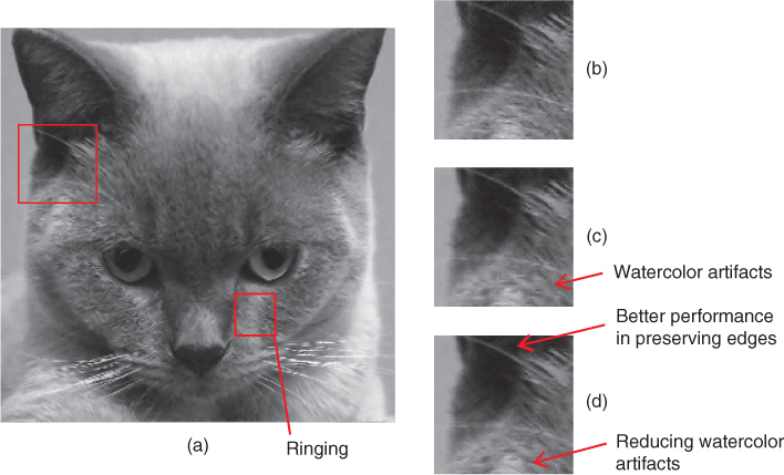
Figure 8.13
A 
 MEDI interpolated Cat image with periodic boundary extension at
  and
and  (PSNR = 27.8014 dB, SSIM = 0.8148). (a) The interpolated image, (b) zoom‐in portion of the ear of the original high‐resolution Cat image, (c) zoom‐in portion of the ear of the NEDI interpolated Cat image, and (d) zoom‐in portion of the ear of the MEDI interpolated Cat image.
The MATLAB function medi can be simply invoked by g = medi(f,48,12) for the case of variance threshold set at ![]() and with boundary width of 12 pixels. To remedy the boundary problem associated with the MEDI kernel, the boundary extension method as discussed in Section 8.4 can be applied. The MEDI interpolated Cat image with variance threshold set at
and with boundary width of 12 pixels. To remedy the boundary problem associated with the MEDI kernel, the boundary extension method as discussed in Section 8.4 can be applied. The MEDI interpolated Cat image with variance threshold set at ![]() with periodic boundary extension to handle boundary pixel problems is shown in Figure 8.13 a, which is obtained with the following function call.
with periodic boundary extension to handle boundary pixel problems is shown in Figure 8.13 a, which is obtained with the following function call.

MEDI has improved the interpolation by modifying geometric structure prediction windows, mean covariance windows, and local covariance windows for type 1 and type 2 pixels, where only the low‐resolution image pixels are considered in those windows, such that the prediction errors aroused in the course of the prediction of type 0 pixels will not propagate to the prediction of type 1 and type 2 pixels. The improvement can be more easily observed by studying the zoom‐in portion of the ear of the Cat image shown in Figure 8.13 d, where the same portion taken from the original image and the NEDI interpolated image are shown in Figures 8.13 b,c, respectively. It can be observed in Figure 8.13 d that the hairs at the upper part of the image are well preserved when compared with that of the NEDI, where more solid and sharp hairs are observed. The MEDI improves the prediction accuracy for type 1 and type 2 pixels, thus improving the interpolation performance along diagonal edges. It also can be observed that MEDI has successfully suppressed the watercolor artifacts when compared with the interpolated image obtained by NEDI as shown in Figure 8.13 c, which is due to the copying of the image features in between neighboring pixels where the prediction of type 1 and type 2 pixels depends on the prediction results of type 0 pixels. With the modified windows in the MEDI, the prediction of each type of pixels acquires a specific set of low‐resolution pixels, thus confining the image features to be interpolated within a predefined region. However, due to the larger size of the modified windows, any image features with size smaller than that of the windows would not be able to be well described by the covariance structure in the windows, thus resulting in local oscillation, which is also known as the ringing artifacts. It can be observed in Figure 8.13 a that the face of the Cat image is degraded by ringing artifacts when compared with that obtained by NEDI (see Figure 8.10 a).
Table 8.2 The PSNR and SSIM performance of a ![]() Cat image interpolation to size
Cat image interpolation to size ![]() using the MEDI and periodic extension with various variance threshold values.
using the MEDI and periodic extension with various variance threshold values.
|
Variance threshold |
PSNR (dB) | SSIM |
| 0 | 27.7930 | 0.8140 |
| 10 | 27.7942 | 0.8143 |
| 48 | 27.8014 | 0.8148 |
| 100 | 27.8082 | 0.8138 |
| 128 | 27.8125 | 0.8133 |
| 200 | 27.8204 | 0.8118 |
| 1000 | 27.8486 | 0.8034 |
| 5000 | 27.4806 | 0.7977 |
|
|
27.3750 | 0.7983 |

Figure 8.14
The zoom‐in portion of the ear of the MEDI interpolated Cat image subject to different thresholds, namely, (a)  , (b)
, (b)  , and (c)
  , where the boundary extension in all images is
  .
.
Besides the subjective evaluation, let us also investigate the objective performance of the MEDI with respect to different values of ![]() . A summary of the PSNR and SSIM performance of the MEDI interpolated Cat image with different
. A summary of the PSNR and SSIM performance of the MEDI interpolated Cat image with different ![]() is shown in Table 8.2 . It can be observed that the PSNR performance of the MEDI is generally improved when compared with that of the NEDI with
is shown in Table 8.2 . It can be observed that the PSNR performance of the MEDI is generally improved when compared with that of the NEDI with ![]() , however the NEDI performs better in PSNR when
, however the NEDI performs better in PSNR when ![]() is further increased. It is because the prediction error propagation is suppressed with the use of modified windows, which reduces the errors across the entire image, especially in improving the prediction accuracy along edges, thus increasing the PSNR. When further increasing the
is further increased. It is because the prediction error propagation is suppressed with the use of modified windows, which reduces the errors across the entire image, especially in improving the prediction accuracy along edges, thus increasing the PSNR. When further increasing the ![]() , more pixels would be interpolated by mean averaging in both the NEDI and the MEDI. However, it is more difficult to preserve the image structure with the large window size of the MEDI after the mean averaging operation (resulting blurred and broken edges). As a result, when the variance threshold is very large, the PSNR will decrease. Therefore, it is vivid that there is a trade‐off between the suppression of prediction error in the covariance‐based interpolation and the degradation of image structure in mean averaging of the larger window size in the MEDI. The SSIM is more effective in revealing the image structures embedded in the interpolated image. It is vivid to observe the variation in SSIM against increasing
, more pixels would be interpolated by mean averaging in both the NEDI and the MEDI. However, it is more difficult to preserve the image structure with the large window size of the MEDI after the mean averaging operation (resulting blurred and broken edges). As a result, when the variance threshold is very large, the PSNR will decrease. Therefore, it is vivid that there is a trade‐off between the suppression of prediction error in the covariance‐based interpolation and the degradation of image structure in mean averaging of the larger window size in the MEDI. The SSIM is more effective in revealing the image structures embedded in the interpolated image. It is vivid to observe the variation in SSIM against increasing ![]() . It can be observed that the SSIM in the MEDI interpolated Cat image turns out to be decreasing when
. It can be observed that the SSIM in the MEDI interpolated Cat image turns out to be decreasing when ![]() is greater than 48, while the PSNR is still increasing. In other words, the image structure degradation brought by mean averaging begins to dominate the interpolation when
is greater than 48, while the PSNR is still increasing. In other words, the image structure degradation brought by mean averaging begins to dominate the interpolation when ![]() is large, which affects the objective performance of the MEDI. Figure 8.14 shows the zoom‐in of the ears of the Cat image taken from the MEDI interpolated images with different thresholds
is large, which affects the objective performance of the MEDI. Figure 8.14 shows the zoom‐in of the ears of the Cat image taken from the MEDI interpolated images with different thresholds ![]() and with the same boundary extension of
and with the same boundary extension of ![]() . It is vivid that the sharpness of the hairs (long edges) is best preserved in the case of
. It is vivid that the sharpness of the hairs (long edges) is best preserved in the case of ![]() . Subject to this
. Subject to this ![]() , the suppression of prediction errors by adopting enlarged windows is the most effective, and the image structure degradation in smooth region brought by mean averaging operation can be alleviated. However, with increasing
, the suppression of prediction errors by adopting enlarged windows is the most effective, and the image structure degradation in smooth region brought by mean averaging operation can be alleviated. However, with increasing ![]() , more ringing artifacts are observed in the interpolated image due to the degraded image feature regulation under a large window size. In other words, the assumption of local stationary is less efficient with increased window size, though the interpolation is still a combination of the covariance‐based interpolation and nonadaptive mean averaging interpolation. By further increasing
, more ringing artifacts are observed in the interpolated image due to the degraded image feature regulation under a large window size. In other words, the assumption of local stationary is less efficient with increased window size, though the interpolation is still a combination of the covariance‐based interpolation and nonadaptive mean averaging interpolation. By further increasing ![]() , the nonadaptive mean averaging interpolation takes over almost all the estimation of the unknown pixels; thus the image features are blurred especially with large window, which results in degradation in both subjective and objective (PSNR and SSIM) measures in the MEDI interpolated images when compared with that of the NEDI results.
, the nonadaptive mean averaging interpolation takes over almost all the estimation of the unknown pixels; thus the image features are blurred especially with large window, which results in degradation in both subjective and objective (PSNR and SSIM) measures in the MEDI interpolated images when compared with that of the NEDI results.
8.7 Covariance Window Adaptation
Another situation where local image blocks do not follow local stationary can be demonstrated by the oversimplified image block example shown in Figure 8.15 . Shown in Figure 8.15 a is a local image block containing two edges (“Edge 1” and “Edge 2”). When the NEDI is applied to interpolate the gray pixel in the center of Figure 8.15 a, the pixels within the box will form the prediction window, and the dashed box will form the mean covariance window. Figure 8.15 b redraws the pixels within the prediction window, which clearly shows that it contains one edge (part of “Edge 1”) only. Shown in Figure 8.15 c are the pixels contained by the mean covariance window, which clearly shows that it contains “Edge 1” and part of “Edge 2.” It is vivid that the covariance structure of the prediction window will not match with the covariance structure of the local image blocks within the mean covariance window. This covariance mismatch violates the geometric duality assumption between the high‐ and low‐resolution images.
As a result, the NEDI interpolated image block will have large interpolation error and undesirable interpolation artifacts. A careful investigation will find that there are two problems associated with the above covariance mismatch interpolation fallacies. The first problem is related to the structure of the windows, while the second one is about the spatial location of the windows relative to the pixel under interpolation.

Figure 8.15 Illustration of covariance mismatch between prediction window and local covariance window corresponding to the gray pixel in (a); (b) prediction window contains Edge 1 only; (c) mean covariance window contains both Edge 1 and Edge 2.
8.7.1 Prediction Window Adaptation
One of the reasons leading to the covariance mismatch of the NEDI is the application of fixed window structure, both size and shape. As a result, one of the remedies is to modify the window to enclose the major feature only, such as to ensure that the low‐resolution image and high‐resolution image have similar covariance structures. Shown in Figure 8.16 are the modified prediction windows with the associated window shapes directed by the edge features within the local region [68 ]. There are four different sets of prediction windows adapting to edges with ![]() ,
, ![]() ,
, ![]() , and
, and ![]() orientations as shown in the figure. The directionality of the prediction window is obtained by elongating the prediction window along the predefined edge direction and narrowing the prediction window in perpendicular to the predefined edge direction. Such window structures can partially alleviate the covariance mismatch problem and slightly improve the objective performance of the interpolated image. However, a lot of image features do not perfectly lie on
orientations as shown in the figure. The directionality of the prediction window is obtained by elongating the prediction window along the predefined edge direction and narrowing the prediction window in perpendicular to the predefined edge direction. Such window structures can partially alleviate the covariance mismatch problem and slightly improve the objective performance of the interpolated image. However, a lot of image features do not perfectly lie on ![]() ,
, ![]() ,
, ![]() , and
, and ![]() (such as in the case of “Edge 1” in Figure 8.15 ). It can foresee that such image feature will not be completely enclosed by any one of the modified prediction windows in Figure 8.16 , and hence the covariance mismatch problem remains. Directional windows that are spatially “wide” in shape are required to accommodate edge features that are not straightly straight line in shape. Another problem of the prediction window is the variation in size to accommodate edges in different sizes and orientations. As a window where the covariance estimation is biased, it will cause the covariance threshold to fail on detecting weak horizontal and vertical edges and falsely detect edge features as
(such as in the case of “Edge 1” in Figure 8.15 ). It can foresee that such image feature will not be completely enclosed by any one of the modified prediction windows in Figure 8.16 , and hence the covariance mismatch problem remains. Directional windows that are spatially “wide” in shape are required to accommodate edge features that are not straightly straight line in shape. Another problem of the prediction window is the variation in size to accommodate edges in different sizes and orientations. As a window where the covariance estimation is biased, it will cause the covariance threshold to fail on detecting weak horizontal and vertical edges and falsely detect edge features as ![]() and
and
![]() . In other words, the consistency of prediction window shape is also important to the performance of the covariance‐based image interpolation algorithm. Shown in Figure 8.17 is one of such prediction window structures.
. In other words, the consistency of prediction window shape is also important to the performance of the covariance‐based image interpolation algorithm. Shown in Figure 8.17 is one of such prediction window structures.

Figure 8.16
Directional adaptive prediction windows with elongation along the edge direction but reducing the width in perpendicular to the edge, where the edge are oriented in  ,
,  ,
,  , and
, and  [68 ].
Visually it is vivid that the arrow‐shaped prediction windows in Figure 8.17 are consistent in shape and are directionally adaptive. Analytically the directional adaptation of the arrow‐shaped prediction windows is obtained from the bias in covariance estimation provided by the spatial orientation of the windows. To determine which window should be applied, the intensity difference of each pair of pixels within each window is computed. The pixel pair with the largest intensity difference will decide the orientation of the edge, and the window that aligns with that pixel pair should be applied. In other words, the prediction window will only contain one pixel pair that are determined to be an edge and hence preserve the geometric regularity of the covariance estimation.

Figure 8.17 Directional adaptive prediction windows that are spatially “wide” in shape: (a) original prediction window and (b)–(e) the modified arrow‐shaped prediction windows in different orientations but in the same size [68 ].
The prediction window adaptation does has its own drawback. Firstly, it is computationally expensive, as additional computations have to be performed to determine which prediction window should be applied. These additional computations are required to estimate the existence of an edge and the orientation of the edge should it exist. The determination of edge feature in these additional computations is a much worst problem than the edge detection problem discussed in Section 2.5 where the detector kernel size is small and hence the detection result is spatially accurate and is not susceptible to low noise level. On the other hand, the problem considered by the selection of prediction window has a much larger kernel size, and hence the result is highly susceptible to image noise. Secondly, the size adapted window does not resolve the problem of completely enclosing short featured image structure (short edge). In this case, the image structure within the covariance estimation window cannot be considered to be locally stationary.
8.7.2 Mean Covariance Window Adaptation
The prediction window adaptation will select a mean covariance window that covers only one image feature in the local image region. The adaptation of the prediction window ponders our question on adapting the mean covariance window to resolve the feature size problem, where the mean covariance window should cover one and only one image feature. As a result, using mean covariance window with size that is too large will capture features that should not coexist in the mean covariance window and the prediction window. However, if the mean covariance window size is too small, it will violate the assumption of local stationary within the mean covariance window. This has led to the development of adaptive window for covariance estimation [5 ]. The interpolation starts from an initial default window size, and the associated interpolation MSE is computed. The interpolation is then performed with a bigger mean covariance estimation window. If the interpolation MSE obtained from bigger mean covariance estimation window is smaller than that of smaller covariance estimation window, the one that achieves the smaller MSE will be adopted. The interpolation will keep performing with larger and larger mean covariance window size until a predefined maximum window size is achieved. The con of this method is the increase in computational complexity because of the iterative nature of the algorithm. The pro is that better interpolated image in both objective and subjective qualities is expected. The reality is that the quality of the image interpolated by this method varies. This is because the estimation of the MSE in the middle of each iteration will determine the performance of the final interpolated image, which is difficult to obtain accurately, if not impossible to obtain at all. Furthermore, increasing the size of the mean covariance window will seldom be locally stationary. The larger the mean covariance window, the more likely more than one image feature will be included within the window, hence implying nonstationary. As a result, the selection of mean covariance window size is an engineering trade‐off between the preservation of covariance structure and the preservation of local stationary (which forms the basis of the geometric duality‐based interpolation).
Furthermore, the nonsymmetrical shape of the mean covariance window makes it directionally sensitive, just like the case of the prediction window. A simple solution to remedy the directional biasing problem of the mean covariance window is to use a circular window as that shown in Figure 8.18 , which was proposed in [5 ]. Enhanced image interpolation results have been observed with this circular mean covariance window that is perfectly circular and has no directionality. The mirror has two faces; however, losing the directionality will require a large window to capture all the edge features inside the window to allow covariance‐based image interpolation. As a result, the same old problem of nonstationary with large window size will pop out.

Figure 8.18 Windows of iNEDI [5 ], where the solid line windows are the low‐resolution window and the dashed line windows is the mean covariance window.
The perfect solution to the question requires a small mean covariance window that can enclose the local image feature (edge) and is unbiased directionally. At the same time, it should allow the covariance‐based interpolation to exploit directional property of the image features enclosed within the mean covariance window for better image interpolation results. These requirements seem contradicting but somehow [59 ] proposed a mean covariance window generation and selection strategy that can almost perfectly achieve the above requirements.
8.7.3 Enhanced Modified Edge‐Directed Interpolation (EMEDI)
To understand how to remedy the covariance mismatch problem, let us first review the problem using Figure 8.19 . Figure 8.19 a shows the prediction window and the mean covariance window adopted in the NEDI. If we allow the mean covariance window to vary its spatial location, we shall observe at least four different poses for the mean covariance windows with reference to the prediction window as shown in Figure 8.19 b–e. These four mean covariance windows are displacement of the original covariance window where the center of the mean covariance window moves from ![]() (the interpolation pixel coordinate) to
(the interpolation pixel coordinate) to ![]() for each pixel on the original mean covariance window indexed by the variable
for each pixel on the original mean covariance window indexed by the variable k. In all the cases, the mean covariance window does completely enclose the prediction window. These displaced mean covariance window placements have achieved different spatial biased, which provide estimation with directionality (similar to that in Figure 8.17 ). At the same time, they are unbiased covariance estimator when compared with each other, because they all have the same shape and are related to each other with a given rotation. Figure 8.20 illustrates the unbiased mean covariance window locations in our example. Among all the mean covariance estimation window, we should choose the one that can achieve the minimal covariance mismatch. Visually we can determine that the mean covariance window in Figure 8.19 e will give the minimal covariance mismatch for the example in Figure 8.19 . Analytically, the search for the best mean covariance window can be achieved by searching for the one that contains the strongest feature (edge). In other words, the search should be performed by computing the total energy of the covariance of each mean covariance window, which is given by
where cov is the covariance operator for the 2D matrix and the ![]() is a per‐matrix element operation. MATLAB has a similar covariance computation function with the same name. The covariance matrix
is a per‐matrix element operation. MATLAB has a similar covariance computation function with the same name. The covariance matrix ![]() is defined in the same way as that in the NEDI algorithm. The total energy of the covariance matrix can be computed by simple MATLAB manipulation. An example of the MATLAB code is shown as below:
is defined in the same way as that in the NEDI algorithm. The total energy of the covariance matrix can be computed by simple MATLAB manipulation. An example of the MATLAB code is shown as below:
![]()

Figure 8.19 Illustration of different placements of covariance estimation window with respect to a fixed prediction window: (a) the placement adopted by the NEDI and (b)–(e) the other four placement variations.
The mean covariance window with the highest mean covariance energy will be selected as the window containing the most significant image feature that would dominate in the linear prediction‐based interpolation. As discussed in the previous section, there could be multiple image features coexisting in a local region. The selection of the mean covariance window with the largest mean covariance energy also makes this type of image block more favorable. This is because the covariance matrix energy reflects the strength of the image feature. The key to remedy the problem of capturing multiple features within the window is to use small window.
Putting them all together the best mean covariance window can be computed with the MATLAB Listing 8.7.1 for a given pixel ![]() with a predefined prediction window displacement matrix
with a predefined prediction window displacement matrix pwin, original mean covariance displacement window mwin, and the local covariance estimation window cwin.

Within each iteration in the for‐loop, the covariance matrix of a biased mean covariance window with center located in one of the original mean covariance window pixel will be constructed with the MATLAB function call to nedi_window, the same covariance matrix construction function used by the NEDI. The total covariance energy of the covariance matrix will be computed and compared with the largest total covariance energy maxE stored so far. If the computed total covariance energy is larger than maxE, it will replace maxE, and the current biased window will temporarily be the best mean covariance window. The mean covariance pixel intensity vector bestwin will be updated to be the pixel intensity of the current biased mean covariance window, such that bestwin=win. The best covariance estimation bestC will also be updated to be the current computed C. The above search will continue until each and every pixel in [m+cwin(1,k),n+cwin(2,k)] has been tested, where in MATLAB a counter parameter wins is defined to realize the parameter ![]() to complete the window definition. This iterative search is initialized with the
to complete the window definition. This iterative search is initialized with the maxE, bestC, and win set to be equal to the total covariance energy, the estimated covariance, and mean covariance window pixel intensity vector of that of the original mean covariance window, respectively.
Figure 8.20 illustrates the spatial adaptation of the mean covariance windows for type 0 pixel, where 5 mean covariance windows are considered in this example. The window indexed by winnum=0 is the original window. While there are four pairs of elements in cwin, there are the additional 4 displaced mean covariance windows (indexed by winnum=1,2,3,and 4) to be considered. This is a simple example showing the basic concept of alleviating the covariance mismatch problem by refining the mean covariance estimation window spatial location subject to the covariance structure carried by the mean covariance estimation window. By biasing the spatial location of the mean covariance estimation window, it effectively enlarges the coverage of the covariance structure estimation spatial area, without actually increasing the kernel size (window size) of the covariance estimation, hence maintaining the local stationary as that of the NEDI. Furthermore, there is no need to modify the shape of the prediction window nor the associated local covariance estimation window (in this example they are both squares in shape as that applied in the NEDI), while still be able to achieve all the benefits of directionality, and space invariant mean covariance estimation window as that in Figures 8.16 –8.18 .

Figure 8.20
Illustration of the spatial adaptation of the five mean covariance windows adopted in the EMEDI for type 0 pixel. Noted the window winnum=0 is same as that in the original NEDI. (See insert for color representation of this figure.)
To implement a covariance‐based image interpolation program that makes use of the best mean covariance window selection, we shall have to insert the function emedi_select_win after the window construction by nedi_window and before the construction of the linear prediction weighting factors by nedi_weighting_factor. The MATLAB function emedi_core listed in Listing 8.7.2 modifies the function nedi_core in Listing 8.3.3 implementing the core function for incorporating local covariance window with maximum covariance power in the interpolation.

This core function can be applied to the same framework as that of the NEDI or the MEDI. In this example, we choose to adopt the MEDI framework to construct the enhanced modified edge‐directed interpolation (EMEDI) image interpolation to demonstrate the progressive interpolation performance improvement from the NEDI to the MEDI and then to the EMEDI. The performance of adopting the NEDI framework for the construction of the EMEDI will be left as an exercise for the readers.
The MATLAB source listed in Listing 8.7.3 implements the EMEDI that is originally proposed by Tam et al. [59 ] and includes the above discussed improvement plus that of the MEDI. The MATLAB function emedi implements a ![]() image interpolation using the EMEDI algorithm with user‐defined threshold
image interpolation using the EMEDI algorithm with user‐defined threshold ![]() and image border width
and image border width b. The threshold will decide whether the weighting factors to be average filtered or to be computed by the covariance based approach depicted in Eq. ( 8.13
), while the image border width will inform the interpolation algorithm how to take care of the image boundary. This is because the kernel size of the covariance estimation window and prediction window is not zero. Therefore, it cannot be applied on the image boundary; otherwise there will be undefined pixels being processed by the window functions. The low‐resolution image is therefore required to perform boundary extension as discussed in Section 2.4.1 such that when operating the EMEDI, the pixel within the extended image border with the width of b will be excluded from the EMEDI operation. The detail of the border extension has been discussed in Section 8.4 .

The MATLAB function emedi can be simply invoked by g = emedi(f,48,20) for the case of threshold set at ![]() and with boundary set at
and with boundary set at ![]() . To remedy the boundary problem associated with the EMEDI kernel, the boundary extension method as discussed in Section 8.4 can be applied. The EMEDI interpolated Cat image with
. To remedy the boundary problem associated with the EMEDI kernel, the boundary extension method as discussed in Section 8.4 can be applied. The EMEDI interpolated Cat image with ![]() and
and ![]() shown in Figure 8.21 a, can be obtained with the following function call.
shown in Figure 8.21 a, can be obtained with the following function call.


Figure 8.21
A 
 EMEDI interpolated Cat image with variance threshold set at
  and with the application of periodic boundary extension (PSNR = 27.8396 dB, SSIM = 0.8147). (a) The interpolated image, (b) zoom‐in portion of the ear of the NEDI interpolated Cat image, (c) zoom‐in portion of the ear of the MEDI interpolated Cat image, and (d) zoom‐in portion of the ear of the EMEDI interpolated Cat image.
The EMEDI interpolated image is shown in Figure 8.21 a. For comparison, the zoom‐in portions of the ear of the Cat image extracted from the NEDI interpolated image, the MEDI interpolated image, and the EMEDI interpolated image are shown in Figure 8.21 b–d, respectively. It can be observed from Figure 8.21 d that the zoom‐in image region of the ear of the Cat image has shown that the EMEDI image interpolation method can better preserve the image structure, when compared with that obtained by the MEDI as shown in Figure 8.21 c. For comparison, the same image region of the NEDI interpoated Cat image is shown in Figure 8.21 b. The EMEDI interpolated image can preserve the image structure better because it adapts the covariance estimation window to the image feature. A larger window area is applied to search for the spatial location that has the highest regularity and hence can preserve the geometric duality better. This is being performed by searching the spatial location of the window with the highest covariance energy. To mitigate the covariance estimation error propagation problem, a bigger window is being adopted in the EMEDI. As a result, all the pixels being applied in the covariance estimation are directly obtained from the low‐resolution image. The con of using a bigger window is the increased ringing artifacts in the interpolated image as observed in Figure 8.21 a. This unwanted ringing artifacts can be suppressed by increasing the threshold ![]() . The side effect of a bigger
. The side effect of a bigger ![]() is more likely that the image edge sharpness will get degraded. The selection of the best
is more likely that the image edge sharpness will get degraded. The selection of the best ![]() is therefore a precise engineering trade‐off problem between the edge sharpness and the ringing artifacts.
is therefore a precise engineering trade‐off problem between the edge sharpness and the ringing artifacts.
Having discussed the pros and cons about the EMEDI and the associated input parameters to the EMEDI, the objective quality of the ![]() interpolated Cat image by the EMEDI has PNSR = 27.8396 dB, which is 0.24 dB better than that of the NEDI, in which the same
interpolated Cat image by the EMEDI has PNSR = 27.8396 dB, which is 0.24 dB better than that of the NEDI, in which the same ![]() is applied. The improvement is attributed to the suppression of the covariance estimation error propagation in the NEDI. Furthermore, the SSIM of the interpolated image obtained by the EMEDI is 0.8147, which is also better than that of the NEDI. The improvement is attributed to the adaptivity of covariance estimation window, such that it can better preserve the covariance structure and hence the geometric duality between the low‐ and high‐resolution image. Table 8.3 shows the summary of the PSNR and SSIM of the EMEDI interpolated images with the same boundary width but different threshold
is applied. The improvement is attributed to the suppression of the covariance estimation error propagation in the NEDI. Furthermore, the SSIM of the interpolated image obtained by the EMEDI is 0.8147, which is also better than that of the NEDI. The improvement is attributed to the adaptivity of covariance estimation window, such that it can better preserve the covariance structure and hence the geometric duality between the low‐ and high‐resolution image. Table 8.3 shows the summary of the PSNR and SSIM of the EMEDI interpolated images with the same boundary width but different threshold ![]() . To further improve the SSIM, the covariance structure between the low‐ and high‐resolution images should be better preserved, which in turn requires a low decision threshold
. To further improve the SSIM, the covariance structure between the low‐ and high‐resolution images should be better preserved, which in turn requires a low decision threshold ![]() value, and hence new methods must be developed to suppress the increased ringing artifacts due to the use of small
value, and hence new methods must be developed to suppress the increased ringing artifacts due to the use of small ![]() . However, small
. However, small ![]() will make the EMEDI to consider weak edges or image noise as strong edges, and applies covariance‐based interpolation on them, thus resulting in unpleasant subjective performance and degrading the PSNR result. In these circumstances, the greater the
will make the EMEDI to consider weak edges or image noise as strong edges, and applies covariance‐based interpolation on them, thus resulting in unpleasant subjective performance and degrading the PSNR result. In these circumstances, the greater the ![]() , the better the PSNR. Therefore, the maxima of PSNR and SSIM as a function of threshold
, the better the PSNR. Therefore, the maxima of PSNR and SSIM as a function of threshold ![]() are not collided, and they are image dependent, which should be carefully chosen. The next section will discuss how to improve the EMEDI through better preservation of covariance structure between the low‐ and high‐resolution images by iterative error correction similar to those presented in Sections 5.6 and 6.4.
are not collided, and they are image dependent, which should be carefully chosen. The next section will discuss how to improve the EMEDI through better preservation of covariance structure between the low‐ and high‐resolution images by iterative error correction similar to those presented in Sections 5.6 and 6.4.
Table 8.3 The PSNR and SSIM performance of a ![]() Cat image interpolation to size
Cat image interpolation to size ![]() using the EMEDI and periodic extension with various variance threshold values.
using the EMEDI and periodic extension with various variance threshold values.
|
Variance threshold |
PSNR (dB) | SSIM |
| 0 | 27.8350 | 0.8142 |
| 48 | 27.8396 | 0.8147 |
| 100 | 27.8414 | 0.8135 |
| 128 | 27.8428 | 0.8128 |
| 200 | 27.8465 | 0.8114 |
| 1000 | 27.8740 | 0.8027 |
| 5000 | 27.5751 | 0.7988 |
|
|
27.3750 | 0.7977 |
8.8 Iterative Covariance Correction
The covariance‐based image interpolation, either the NEDI, the MEDI, or the EMEDI, is developed with the assumption of geometric duality between the low‐ and high‐resolution images. It has been demonstrated in previous sections that even if the local image block within the covariance estimation window is locally stationary and regular, the local image block obtained from the NEDI, the MEDI, and the EMEDI interpolations will not have the same covariance structure as that of the low‐resolution image block. There are a lot of reasons on the inefficiency of the interpolation algorithm such that the obtained local image block does not have the same covariance structure as that of the low‐resolution image. One of the reasons will be that the interpolated pixel is obtained as the least squares solution of the estimated covariance structure, which is known to be sensitive to outliers, where we refer the outliers to noises in the image. A number of intermediate solutions have been presented in literature trying to remedy this poor estimation problem. The robust NEDI [42 ] incorporated a nonlocal mean method to optimize the linear prediction interpolation results, where the similarity of neighboring windows is compared with that of the current prediction window. When the covariance structure of the prediction window under concern is found to be similar to that of the neighboring windows, the prediction coefficients obtained from the original covariance estimation window and its neighboring windows with similar covariance structure will be mean filtered. The image obtained from these mean filtered prediction coefficients has found to be robust to image noises and be able to provide interpolated images with better objective and subjective qualities. However, similar to choosing a larger ![]() to avoid noise being considered as image features, the mean filtered prediction will also cause degradation of structural details.
to avoid noise being considered as image features, the mean filtered prediction will also cause degradation of structural details.

Figure 8.22 Illustration of the examples of the biased covariance windows for high‐ and low‐resolution image pixels.
Before we can find a way to improve the local region of the high‐resolution image to attain the same covariance structure as that of the corresponding low‐resolution image region, we shall have to quantify the meaning of covariance difference analytically. The covariance structure difference between the covariance matrices of the corresponding low‐ and high‐resolution image regions may not be compatible in dimension. As a result, we compare the total energy of the low‐ and high‐resolution covariance matrices similar to that in Section 8.7.3 . In particular, we shall compare the total energy of the low‐resolution covariance matrix with the corresponding high‐resolution covariance matrices under spatial displacements. The reason is the same as that discussed in Section 8.7.3 , such that we shall allow the high‐resolution covariance estimation to be spatially biased to capture the structure of the image feature for better preservation of the structural regularity. Given an interpolated pixel coordinate at [m,n], the spatial coordinates of the corresponding low‐resolution image block are given by [m+lwin(1,:),n+lwin(2,:)] with the low‐resolution pixel window spatial displacement vector lwin given by

for type 0 pixels. This particular choice of low‐resolution window, which is the winnum=0 mean covariance window in Figure 8.20 surrounding the pixel to be interpolated, is shown in Figure 8.22 . This specific window forms a fourth‐order window with only the ![]() low‐resolution pixels (dark pixels) being considered. The second and third windows surrounding the interpolated pixel are not chosen because the second window containing only four low‐resolution pixels is too small to capture image features, while the third window will include pixels from both high‐ and low‐resolution images and hence does not fulfill our purpose. Similarly, the displacement vector
low‐resolution pixels (dark pixels) being considered. The second and third windows surrounding the interpolated pixel are not chosen because the second window containing only four low‐resolution pixels is too small to capture image features, while the third window will include pixels from both high‐ and low‐resolution images and hence does not fulfill our purpose. Similarly, the displacement vector hwin specifies the spatial coordinate displacement of the prediction window to extract the high‐resolution pixel window, which forms a third‐order system that covers ![]() pixels surrounding the pixel to be interpolated, in which both low‐ and high‐resolution pixels are considered. It is the difference in the order that makes direct comparison between the two covariance matrices impossible. We can either change the window size, or we can compare their total energy, and in this section we choose the latter one, which is also the easier one. The spatial coordinates for the high‐resolution image block biased to the
pixels surrounding the pixel to be interpolated, in which both low‐ and high‐resolution pixels are considered. It is the difference in the order that makes direct comparison between the two covariance matrices impossible. We can either change the window size, or we can compare their total energy, and in this section we choose the latter one, which is also the easier one. The spatial coordinates for the high‐resolution image block biased to the ![]() th prediction pixels
th prediction pixels pwin(:,k) are given by [m+pwin(1,k)+hwin(1,:),n+pwin(2,k)+hwin(2,:)]. The corresponding lwin and hwin for type 1 pixels are given by

and for type 2 pixels

Once the image block pixel coordinates are constructed, the low‐ and high‐resolution image intensity vectors LRblk and HRblk, respectively, can be obtained by the following MATLAB code:
![]()
the total covariance energy of these image blocks are obtained with function call to cov

Now we can algorithmically define the covariance difference as
![]()
We can put the above together to form imedi_select_win in Listing 8.8.1 to select the biased high‐resolution prediction window that can achieve the smallest covariance difference.

The function imedi_select_win is similar to emedi_select_win in Listing 8.7.1, where emedi_select_win adapts the mean covariance window, while imedi_select_win adapts the high‐resolution prediction window. The biased high‐resolution prediction window that can achieve the smallest covariance difference will be selected. If, for example, the smallest covariance difference is achieved by the ![]() th biased high‐resolution prediction window, prediction window should be displaced. However, for the purpose of implementation, it is easier to displace the interpolated pixel location from
th biased high‐resolution prediction window, prediction window should be displaced. However, for the purpose of implementation, it is easier to displace the interpolated pixel location from [m,n] to [m+cwin(1,k),n+cwin(2,k)] and hence the last if‐else command in the MATLAB Listing 8.8.1. The imedi_select_win will return the pixel intensity vectors of the best selected mean covariance window bestwin and prediction window bestxLR and the associated covariance matrix bestC. These information will be fed into nedi_weighting_factor to generate the linear prediction coefficients, and so is the intensity of the pixel to be interpolated, in the same manner as that of the NEDI. The improved method is named
improved modified edge‐directed interpolation
(iMEDI). All of these are implemented in the core function imedi_core in Listing 8.8.2, which will return the intensity of the interpolated pixel that achieves the minimal covariance difference.

A similar framework as that of emedi in Listing 8.7.3 is applied to implement the iMEDI interpolation in MATLAB source Listing 8.8.3.

Unlike nedi, medi, and emedi, the MATLAB function imedi does not interpolate image. Instead, the following function call
![]()
takes in a high‐resolution image g and generates another image g1 with the same resolution, where the pixels corresponding to the down‐sampled version of g are preserved, while other pixels are interpolated to minimize the covariance difference between that of the down‐sampled images. The rest of the parameters are defined to be the same as that in nedi. To smooth out the covariance difference problem, mean filtering should be applied to g1 and g, such as
![]()
which is known as dyadic averaging. If the mean filtered image is considered to be still suffering from covariance difference problem, the imedi can be invoked again, and another mean filtering can be performed. However, iterative application of dyadic averaging is biased to the last generated image and minimized the contribution from the first image. The equal weighting average should be applied in iterative covariance difference minimization that uses imedi to generate multiple high‐resolution images in for‐loop. As an example, at the ![]() th loop that generates the
th loop that generates the ![]() th high‐resolution image
th high‐resolution image g1 from the ![]() th equal averaged image
th equal averaged image g, the equal weighting average image will be obtained as
![]()
Finally the iterative covariance difference minimization procedure is implemented with the MATLAB function imediloop in Listing 8.8.4 with details to be presented in the next section.
8.8.1 iMEDI Implementation
Putting them all together, the MATLAB function imediloop listed in Listing 8.8.4 implements a ![]() image interpolation which iteratively minimizes the covariance difference of the interpolated high‐resolution image obtained by
image interpolation which iteratively minimizes the covariance difference of the interpolated high‐resolution image obtained by medi with respect to the given low‐resolution image.

The parameters in imediloop are defined to be the same as those in nedi. There are two newly added parameters, tc and i. The iterative covariance difference minimization will stop when the number of iteration equals i. The iteration will also come to a premature stop when the absolute difference of the mean squares difference between the mean filtered high‐resolution images obtained at the ![]() th iteration and that obtained at the
th iteration and that obtained at the ![]() th iteration is smaller than the predefined threshold
th iteration is smaller than the predefined threshold tc. To compute the mean squares difference between two high‐resolution images, the following MATLAB function cmse is created, which will take in the original high‐resolution image oimg and the processed high‐resolution image rimg and return the mean squares difference between these two images. In other words, the ![]() th iteration image and the
th iteration image and the ![]() th image would be considered as
th image would be considered as oimg and rimg, respectively.
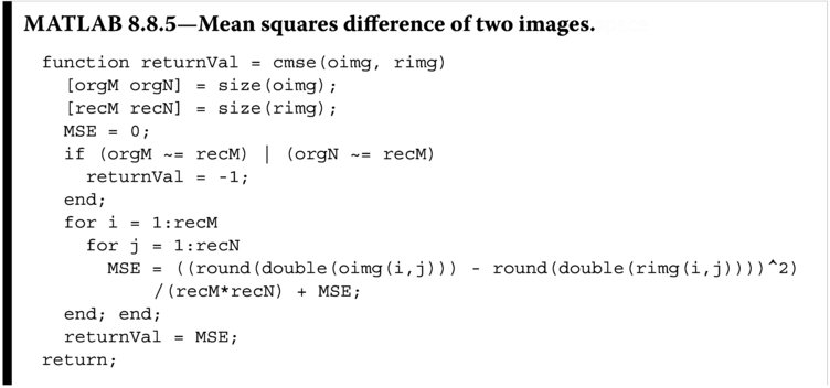
The ![]() interpolated Cat image shown in Figure 8.23 a is obtained with the following function call to
interpolated Cat image shown in Figure 8.23 a is obtained with the following function call to imediloop:
![]()

Figure 8.23
iMEDI interpolation of the Cat image by a factor of 2 and with threshold  (PSNR = 27.9552 dB, SSIM = 0.8201) with five iterations: (a) the interpolated image, (b) zoom‐in portion of the ear of the NEDI interpolated Cat image, (c) the EMEDI interpolated Cat image, and (d) the sixth iteration iMEDI interpolated Cat image.
The above parameters are for ![]() , image boundary width of 20, and a maximum of 10 iterations of covariance corrections with premature stop when the difference of the images in consecutive iteration measured by mean squares error is smaller than 0.1. For the Cat image with chosen
, image boundary width of 20, and a maximum of 10 iterations of covariance corrections with premature stop when the difference of the images in consecutive iteration measured by mean squares error is smaller than 0.1. For the Cat image with chosen ![]() ,
, ![]() , and
, and ![]() , the iteration stops at the sixth iteration. It can be observed from the zoom‐in image block of the ear of the Cat image shown in Figure 8.23 d that taken from the iMEDI final image obtained at the sixth iteration, it can preserve the image structure better when compared with that obtained by the EMEDI as shown in Figure 8.23 c. For comparison, the same image block of the NEDI interpolated Cat image is shown in Figure 8.23 b. The covariance correction in the iMEDI helps to preserve the image structure of the interpolated image to be almost the same as that of the low‐resolution image. As a result, the edges are sharp, and the very few ringing nor checkerboard noises are observed in the interpolated image when compared with that obtained from the EMEDI and the NEDI. Both subjective and objective qualities of the sixth iteration iMEDI interpolated image are better than that of the EMEDI and the NEDI, where the PSNR equals 27.9552 dB, which is 0.1156 dB higher than that of the EMEDI, which achieves the best PSNR among all three methods. Moreover, the SSIM equals 0.8201, which is 0.0054 higher than that obtained by the EMEDI. This observation shows that the iterative error correction method can successfully improve the structure regularity of the covariance‐based interpolation method.
, the iteration stops at the sixth iteration. It can be observed from the zoom‐in image block of the ear of the Cat image shown in Figure 8.23 d that taken from the iMEDI final image obtained at the sixth iteration, it can preserve the image structure better when compared with that obtained by the EMEDI as shown in Figure 8.23 c. For comparison, the same image block of the NEDI interpolated Cat image is shown in Figure 8.23 b. The covariance correction in the iMEDI helps to preserve the image structure of the interpolated image to be almost the same as that of the low‐resolution image. As a result, the edges are sharp, and the very few ringing nor checkerboard noises are observed in the interpolated image when compared with that obtained from the EMEDI and the NEDI. Both subjective and objective qualities of the sixth iteration iMEDI interpolated image are better than that of the EMEDI and the NEDI, where the PSNR equals 27.9552 dB, which is 0.1156 dB higher than that of the EMEDI, which achieves the best PSNR among all three methods. Moreover, the SSIM equals 0.8201, which is 0.0054 higher than that obtained by the EMEDI. This observation shows that the iterative error correction method can successfully improve the structure regularity of the covariance‐based interpolation method.
Table 8.4 The PSNR and SSIM performance of a ![]() Cat image interpolation to size
Cat image interpolation to size ![]() using the iMEDI and periodic extension with various variance threshold values
using the iMEDI and periodic extension with various variance threshold values
|
Variance threshold |
Total number of iMEDI iterations | PSNR (dB) | SSIM |
| 0 | 6 | 27.9542 | 0.8203 |
| 48 | 6 | 27.9552 | 0.8201 |
| 100 | 6 | 27.9557 | 0.8184 |
| 1000 | 7 | 27.9010 | 0.8038 |
| 5000 | 4 | 27.4910 | 0.7984 |
|
|
1 | 27.3750 | 0.7977 |
Similar to all other covariance‐based image interpolation algorithms, the performance of imediloop is ![]() sensitive. Listed in Table 8.4 are the PSNR and SSIM of the
sensitive. Listed in Table 8.4 are the PSNR and SSIM of the ![]() interpolated Cat image obtained with various threshold
interpolated Cat image obtained with various threshold ![]() values. It can be observed from the table that the PSNR and SSIM do not seem to agree with each other in this example. The PSNR of the
values. It can be observed from the table that the PSNR and SSIM do not seem to agree with each other in this example. The PSNR of the imediloop interpolated Cat image achieves its highest value at ![]() , while the SSIM achieves its highest value at
, while the SSIM achieves its highest value at ![]() . This might be due to the fact that the Gaussian smoothing applied to compute SSIM (readers please refer to Section 3.3) has blurred the perfectly captured image features and hence compromised the SSIM value. Readers should also be able to observe from Table 8.4 and other tables in 8.1 , 8.2 , and 8.3 that the influence of
. This might be due to the fact that the Gaussian smoothing applied to compute SSIM (readers please refer to Section 3.3) has blurred the perfectly captured image features and hence compromised the SSIM value. Readers should also be able to observe from Table 8.4 and other tables in 8.1 , 8.2 , and 8.3 that the influence of ![]() value on the final image quality is not as huge as that in the cases of the EMEDI, the MEDI, and the NEDI. This robustness is the result of the iterative covariance difference minimization. It can be observed that a satisfactory threshold immunity can be achieved when the number of iteration is more than 6 for the Cat image.
value on the final image quality is not as huge as that in the cases of the EMEDI, the MEDI, and the NEDI. This robustness is the result of the iterative covariance difference minimization. It can be observed that a satisfactory threshold immunity can be achieved when the number of iteration is more than 6 for the Cat image.
The first row in Figure 8.24 shows the normalized covariance energy difference maps for the iMEDI interpolated image taken from the third, the fifth, and the sixth iterations. The covariance energy difference maps are obtained by computing the difference in the total covariance energy in the lwin and the hwin windows. To show vivid variation in the energy difference maps, only the pixels on the difference maps where actual interpolated pixels exist will be considered, and those coupled to pixels inherited from original low‐resolution image will be discarded. Moreover, the energy difference maps taken from different iterations are converted into logarithmic scale and normalized by the built‐in MATLAB function mat2gray into the range of [0, 1] all together, such that the intensity variation in the difference images reflects the variation in energy difference among all the three cases. It should be noted that the brighter the intensity of the pixels in Figure 8.24 , the greater the energy difference and the lower the correlation between the two windows. It can be observed that the outlines of the Cat become more blurred as the iteration goes, which indicates that the covariance energy difference along image edges and features is reducing. This attributes to the prediction errors in the covariance‐based interpolation along the image edges and features reducing along the iterations. This is also the objective of the iterative approach to minimize the mean squares error of the interpolated image, eventually improving the PSNR.
The second row in Figure 8.24 shows the zoom‐in maps of the selected regions highlighted in the first row, where the region corresponding to the left ear of the Cat image is chosen. It should be noted that instead of directly enlarging the images presented in the first row, the selected regions from each of the difference maps are grouped together and undergone an independent normalization procedure for better comparison purpose. The white regions indicate the error concentrated regions. It can be observed that instead of clear outlines of the hairs as shown in the third iteration result, it becomes many patches stitched together as that shown in the sixth iteration result. Moreover, more dense bright regions are observed in the third iteration result. All these further show the improvement in the structural integrity brought by the iterative approach. To take a closer look of the dense region, the same set of zoom‐in maps is further manipulated that only those pixels with intensity greater 0.85 are kept and presented in the third row in Figure 8.24 . It can be observed that the covariance energy difference pixels are more closely packed with increasing iteration, while more unconnected pixels are observed in the third iteration result, which shows that the better image structure is preserved by increasing the iteration. By investigating the total energy difference in the manipulated maps, the total energy differences are 202.77, 202.79, and 201.93 for the third, fifth, and sixth iteration results, respectively, whereas the peak difference is 0.9996, 0.9999, and 1, respectively. This observation further shows that the iteration approach increases the interpolation errors in localized area but will generally lower the interpolation error in average when it converges.

Figure 8.24 Covariance energy difference maps of the iMEDI interpolated Cat image at (a) the third iteration, (b) the fifth iteration, and (c) the sixth iteration.

Figure 8.25
The iMEDI interpolation suppresses the ringing artifact when compared with that of EMEDI: (a) the EMEDI interpolated Cat image and (d) the iMEDI interpolated Cat image, where the same scaling factor of 2 and threshold  are applied. (b) and (c) are the corresponding zoom‐in portion of the hairs of both interpolated images.
The selection of the best ![]() is important in all covariance‐based edge‐directed image interpolation methods. The subjective image quality between the interpolated images obtained by the iMEDI and the EMEDI is also similar, where the edges are sharp and there are very few artifacts in the interpolated image. Of course, there is minor difference between the texture‐rich regions of the two interpolated images since the lower
is important in all covariance‐based edge‐directed image interpolation methods. The subjective image quality between the interpolated images obtained by the iMEDI and the EMEDI is also similar, where the edges are sharp and there are very few artifacts in the interpolated image. Of course, there is minor difference between the texture‐rich regions of the two interpolated images since the lower ![]() value will invite more texture‐rich region pixels to be interpolated by covariance‐based interpolation, while they should be treated with nonparametric interpolation, such as the bilinear interpolation. Nevertheless, the iMEDI method with multiple iterations can achieve the best image quality. This improvement shows supreme performance in tackling the ringing artifacts in texture‐rich regions, which is well presented in Figure 8.25 . The ringing artifacts on the face of the Cat image in the iMEDI interpolated image are suppressed even when the same
value will invite more texture‐rich region pixels to be interpolated by covariance‐based interpolation, while they should be treated with nonparametric interpolation, such as the bilinear interpolation. Nevertheless, the iMEDI method with multiple iterations can achieve the best image quality. This improvement shows supreme performance in tackling the ringing artifacts in texture‐rich regions, which is well presented in Figure 8.25 . The ringing artifacts on the face of the Cat image in the iMEDI interpolated image are suppressed even when the same ![]() is applied (Figure 8.25 ). Of course the con will be the high computation cost as the low‐resolution image will have to go through multiple covariance‐based image interpolations. However, as a household saying goes, “it is worthy to wait in line for good stuffs.”
is applied (Figure 8.25 ). Of course the con will be the high computation cost as the low‐resolution image will have to go through multiple covariance‐based image interpolations. However, as a household saying goes, “it is worthy to wait in line for good stuffs.”
8.9 Summary
The idea of following edges during image interpolation has been considered in Chapter 7. This chapter discussed an alternative way to perform edge‐directed image interpolation without generating an explicit edge map. The covariance‐based image interpolation methods presented in this chapter are developed with two basic assumptions that a natural image is a second‐order locally stationary Gaussian process and image edges acquire the geometric duality properties. The image features captured by local covariance of small image blocks (also known as the estimation window) are exploited to develop image interpolation algorithm. In particular, the geometric duality between the covariance of localized image block of low‐resolution image and the corresponding high‐resolution image is applied to allow the tuning of interpolation coefficients to match arbitrary oriented image features (edges) to perform a non‐explicit edge‐directed image interpolation. The statistical adaptive approach is able to accurately locate the image edges in all arbitrary orientation, thus preventing the edge mis‐registration problem observed in those edge‐directed interpolation methods using edge map. In particular we have used the NEDI and its variants as examples to present the development of covariance‐based image interpolation methods.
The original NEDI works well and can produce high quality (both subjective and objective quality measures) image interpolation results until the assumptions break down. The assumptions will break down when the NEDI suffers from local stationary, covariance estimation error propagation, and inefficient estimation result that cannot preserve the geometric duality. The former one is caused by the covariance estimation windows being not able to co‐align with the image features. It can also be caused by biased covariance estimation windows. The covariance estimation error propagation problem is caused by using part of the estimation results from pixels obtained in previous estimation for estimating unknown pixel values. As a result, the estimation error between these pixels will be correlated and results in clustered and easily detectable artifacts. The last problem is almost unavoidable due to the fact that low‐resolution image does not contain all the information needed for a perfect estimation. This is also why image interpolation problem is an ill‐posed problem. However, knowing that our objective is to interpolate a high‐resolution image that preserves the geometric regularity of its low‐resolution partner, researcher should come up with innovative solution, whether it is brute force or by other means, to enforce the interpolated image to strictly follow this property.
Various methods to remedy the above weakness of the NEDI algorithm have been discussed in literature and in this chapter. The estimation error propagation problem is tackled by using new estimation window structure that only makes use of the low‐resolution image pixels [59 ], where we have presented the algorithm MEDI and showed that better interpolated images can be obtained when compared with that of the NEDI. To alleviate the local stationary and geometric regularity violation problems, there have been a lot of research works presented in literature, and so far the most effective methods will identify the appropriate covariance estimation window based on the local image covariance structure [59 ], nonlocal image covariance structure [19, 70 ], or resemblance of error minimization filter into the covariance matrix [30, 42 ]. All of these methods estimate the unknown pixel intensities in the same fashion as that of the NEDI, but the definition of the covariance estimation window adapts to the covariance structure of the image, such that it provides a better performance in preserving the local stationary and geometric regularity. In particular, the chapter chose the method presented in [59 ] to demonstrate the development and implementation of covariance‐based image interpolation method with adaptive estimation window, such that the window is spatially adaptive to allow small‐size estimation window that better preserves the local stationary of short edges, and small image features, while also having a large mean covariance estimation window size such as not to miss the existence of image features that constitute the covariance structure for interpolation that preserves the geometric regularity. The presented method is the EMEDI, which is built upon MEDI. Interpolated image with sharper and better edge continuity is observed, besides being able to achieve better objective performance.
The NEDI, MEDI, and EMEDI estimate the unknown pixels from neighboring pixels with optimal weighting factors obtained by linear prediction. The linear prediction is an analysis‐by‐synthesis process that produces the optimal weighting factors by minimizing the mean squares error obtained in prediction through Wiener filtering. Needless to say, prediction error is inevitable. As a result the geometric regularity is not preserved in strict sense. In this chapter we propose to resolve the problem by iterative covariance energy correction, such that the energy of the covariance matrices for all the interpolated pixels is compared with the corresponding energy of the covariance matrices of the low‐resolution image. Should the difference between these two energies be larger than a given threshold, we shall interpolate that particular pixel again using the new covariance matrix obtained in the current high‐resolution image. This will generate a new high‐resolution image, which will be mean filtered with the high‐resolution image in previous iteration to produce the final interpolated image. We demonstrated the implementation of such algorithm through the iMEDI, which is built upon the EMEDI. Better image interpolation results with high objective quality are obtained by the iMEDI interpolated images.
The possible improvement of covariance‐based image interpolation method certainly will not stop here. One of the major improvements over the NEDI‐based covariance‐based image interpolation is the application of Markov random field to perform the interpolation [39 ]. We are glad to share some discussions with Dr. Min Li about developing a chapter in the initial version of this book for her image interpolation method. We feel very sorry that finally her work is not discussed in this book due to time and space restriction. Hopefully we can do that in the next edition of this book. More and more techniques will be developed in the future to produce better and better interpolated images. It is our purpose to show the theory, mathematics, algorithmic derivation, and MATLAB implementation to the readers such that they can make use of the presented information to develop their better and faster covariance‐based image interpolation methods.
8.10 Exercises
- 8.1
The MATLAB function
nedi_correct(Listing 8.3.5) adjusts the pixel intensity of an interpolated pixel to be bounded within the allowable dynamic range defined by the pixel intensity of the pixels in the prediction window via mean value interpolation. Create a functionnedi_correct_bilinearto achieve the adjustment through bilinear interpolation and incorporate it into thenedi. Demonstrate and compare the performance of the newnedialgorithm by interpolating the Cat image. - 8.2 Interpolate the image Cat by the NEDI using different boundary extension methods: (a) by constant extension, (b) by periodic extension, (c) by symmetric extension, and (d) by infinite extension. Compare their subjective and objective performance.
- 8.3
Compare the PSNR and SSIM of the interpolation of Cat image by the NEDI with different
b: (a) , (b)
, (b)  , and (c)
  .
. - 8.4
Compare the subjective and objective performance of the iMEDI with the use of different covariance‐based interpolation methods to generate the initial high‐resolution image by (a) the NEDI and (b) the EMEDI. Compare the number of iterations required for each of them to converge, the subjective performance, PSNR, SSIM, and CMSE of these two approaches using
 and
and  against those of the original
 imediloop. (Hint: Theimediloopfunction [in Listing 8.8.4] generates the initial high‐resolution imagegbymedi.)